SIRIUS project. I. Star formation models for star-by-star simulations of star clusters and galaxy formation
←
→
Page content transcription
If your browser does not render page correctly, please read the page content below
Publ. Astron. Soc. Japan (2021) 00(0), 1–23   1
                                                                                                                                         doi: 10.1093/pasj/xxx000

                                               SIRIUS project. I. Star formation models for
                                               star-by-star simulations of star clusters and
arXiv:2005.12906v2 [astro-ph.GA] 13 Mar 2021

                                               galaxy formation
                                               Yutaka H IRAI1 , Michiko S. F UJII2 and Takayuki R. S AITOH3, 4
                                               1
                                                 RIKEN Center for Computational Science, 7-1-26 Minatojima-minami-machi, Chuo-ku, Kobe,
                                                 Hyogo 650-0047, Japan
                                               2
                                                 Department of Astronomy, Graduate School of Science, The University of Tokyo, 7-3-1
                                                 Hongo, Bunkyo-ku, Tokyo 113-0033, Japan
                                               3
                                                 Department of Planetology, Graduate School of Science, Kobe University, 1-1 Rokkodai-cho,
                                                 Nada-ku, Kobe, Hyogo 657-8501, Japan
                                               4
                                                 Earth-Life Science Institute, Tokyo Institute of Technology, 2-12-1 Ookayama, Meguro-ku,
                                                 Tokyo 152-8551, Japan
                                               ∗ E-mail:   yutaka.hirai@riken.jp, fujii@astron.s.u-tokyo.ac.jp, saitoh@people.kobe-u.ac.jp
                                               Received 2021 March 16; Accepted

                                               Abstract
                                               Most stars are formed as star clusters in galaxies, which then disperse into galactic disks.
                                               Upcoming exascale supercomputational facilities will enable performing simulations of galaxies
                                               and their formation by resolving individual stars (star-by-star simulations). This will substantially
                                               advance our understanding of star formation in galaxies, star cluster formation, and assembly
                                               histories of galaxies. In previous galaxy simulations, a simple stellar population approxima-
                                               tion was used. It is, however, difficult to improve the mass resolution with this approximation.
                                               Therefore, a model for forming individual stars that can be used in simulations of galaxies must
                                               be established. In this first paper of a series of the SIRIUS (SImulations Resolving IndividUal
                                               Stars) project, we demonstrate a stochastic star formation model for star-by-star simulations.
                                               An assumed stellar initial mass function (IMF) is randomly assigned to newly formed stars in
                                               this model. We introduce a maximum search radius to assemble the mass from surrounding
                                               gas particles to form star particles. In this study, we perform a series of N -body/smoothed par-
                                               ticle hydrodynamics simulations of star cluster formations from turbulent molecular clouds and
                                               ultra-faint dwarf galaxies as test cases. The IMF can be correctly sampled if a maximum search
                                               radius that is larger than the value estimated from the threshold density for star formation is
                                               adopted. In small clouds, the formation of massive stars is highly stochastic because of the
                                               small number of stars. We confirm that the star formation efficiency and threshold density do
                                               not strongly affect the results. We find that our model can naturally reproduce the relationship
                                               between the most massive stars and the total stellar mass of star clusters. Herein, we demon-
                                               strate that our models can be applied to simulations varying from star clusters to galaxies for a
                                               wide range of resolutions.
                                               Key words: methods: numerical — ISM: clouds — open clusters and associations: general — galaxies:
                                               formation — galaxies: star clusters: general

                                               © 2021. Astronomical Society of Japan.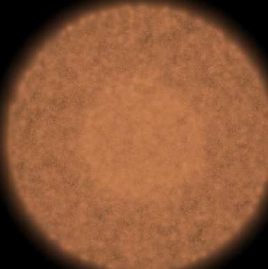
2                                                            Publications of the Astronomical Society of Japan, (2021), Vol. 00, No. 0

1 Introduction                                                    pernova driven winds converged within the simulations,
                                                                  with one gas-particle mass of less than 5 M⊙ . Emerick
Our goal is to gain a comprehensive picture of the                et al. (2019) also computed isolated dwarf galaxies with
formation and evolution of star clusters and galaxies.            star-by-star yields of supernovae. They have shown that
Simulations that can resolve individual stars (hereafter,         the outflows caused by supernova feedback have a larger
star-by-star simulations) of galaxies are expected to pro-        metallicity than that of the interstellar medium (ISM).
vide a breakthrough in studies of galaxy formation. These
                                                                      Exascale computational facilities will make it possible
simulations can assess the formation of star clusters and
                                                                  to perform star-by-star simulations up to the Milky Way
their evolution across the cosmic time (Krumholz et al.
                                                                  mass galaxy scale within the next decade. These facilities
2019). Humanity’s understanding of the assembly histo-
                                                                  are planned in different institutions. The supercomputer
ries of galaxies will be considerably improved by star-by-
                                                                  Fugaku in RIKEN has commenced operation. Oak Ridge
star comparisons with the chemo-dynamical properties of
                                                                  National Laboratory plans to operate the exascale super-
stars obtained from the astrometric satellite Gaia (Gaia
                                                                  computer Frontier in 2021. China plans three projects for
Collaboration et al. 2018), spectroscopic observations with
                                                                  exascale computing. By using such facilities, star-by-star
astronomical telescopes, and simulations. Feedback from
                                                                  simulations with 1011 particles are expected to be possible
supernovae is independent of the models in these high-
                                                                  if code with high-scalability can be developed.
resolution simulations because the latter can detail the evo-
                                                                     A sink particle approach has often been used in rel-
lution of supernova remnants (e.g., Dalla Vecchia & Schaye
                                                                  atively small-scale simulations (e.g., Bate et al. 1995;
2012; Hopkins et al. 2018a; Hu 2019).
                                                                  Bonnell et al. 2003, 2004; Krumholz et al. 2004; Bate
   Galaxies consist of objects with a broad mass range.           & Bonnell 2005; Jappsen et al. 2005; Clark et al. 2005;
The largest objects in the Local Group are M31 and                Federrath et al. 2010; Hubber et al. 2013b; Bleuler &
the Milky Way, as they have a total stellar mass of ∼             Teyssier 2014; Klassen et al. 2016; Gatto et al. 2017;
1011 M⊙ . Conversely, recently discovered ultra-faint dwarf       Shima et al. 2018; Kim et al. 2018a; Fukushima et al.
galaxies have a total stellar mass of only <     5
                                            ∼ 10 M⊙ (e.g.,        2020). Bonnell et al. (2003) performed a series of N -
Simon 2019). Globular clusters and open star clusters also        body/smoothed particle hydrodynamics (SPH) star clus-
have an extensive mass range, from 102 to 107 M⊙ (e.g.,           ter formation simulations from turbulent molecular clouds.
Portegies Zwart et al. 2010). These objects are formed            The mass of one gas particle of their simulation was
within the broader events of galaxy formation. Saitoh             0.002 M⊙ , and their results showed that the hierarchical
et al. (2009) have shown that mergers of galaxies induce          fragmentation of turbulent molecular clouds helped form
the formation of star clusters. Kim et al. (2018b) have also      small star clusters. The merging of these objects formed
identified that the mergers of high-redshift galaxies form        the final star clusters. He et al. (2019) performed a series of
globular cluster-like objects (see also, Ma et al. 2020). To      radiation-magneto-hydrodynamic simulations of star clus-
comprehensively understand their formation and relation-          ters with a spatial resolution of 200 to 2000 au. They
ship to the building blocks of galaxies, it is necessary to       found that the IMF’s observed power-law slope could be
evaluate small star clusters and ultra-faint dwarf galaxies       reproduced if they assumed that 40% of a star-forming
within the formation of more massive galaxies.                    gas clump was converted into the most massive stars, and
   In the last decade, the mass resolution in simulations         others were distributed to the smaller mass stars.
of galaxies has greatly improved (Vogelsberger et al. 2020,          For more massive clusters, ‘cluster particle’ approach is
and references therein). Bédorf et al. (2014) performed          used (Dale et al. 2012, 2014; Sormani et al. 2017; Kim et al.
an N -body simulation of a Milky Way mass galaxy using            2018a; Howard et al. 2018; Wall et al. 2019; He et al. 2019;
1011 particles. Current state-of-the-art hydrodynamic sim-        Fukushima et al. 2020). This is similar to the simple stel-
ulations of Milky Way mass galaxies have reached a mass           lar population (SSP) approximation in galaxy simulations
resolution of less than 104 M⊙ (e.g., Grand et al. 2017;          and cluster particles, containing a bunch of stars following
Hopkins et al. 2018b; Font et al. 2020; Agertz et al. 2020a;      a given mass function. The masses of cluster particles de-
Applebaum et al. 2021). A considerably higher resolu-             pend on the simulation scale and the resolution, but they
tion is possible in simulations of dwarf galaxies (e.g., Hirai    are typically orders of ten to a hundred.
et al. 2015, 2017; Rey et al. 2019; Wheeler et al. 2019;             Sink particle approach is difficult to apply for simula-
Lahén et al. 2019, 2020; Agertz et al. 2020b; Gutcke et al.      tions in a scale of galaxies. Simulations cannot resolve the
2021; Smith 2021). Recently, Hu (2019) performed a se-            formation of the lowest-mass stars even if exascale super-
ries of simulations of isolated dwarf galaxies with a mass        computers are used. At least 1015 particles are required to
resolution of ∼ 1 M⊙ . They showed that properties of su-         resolve the Jeans mass of 0.1 M⊙ with 100 particles, cor-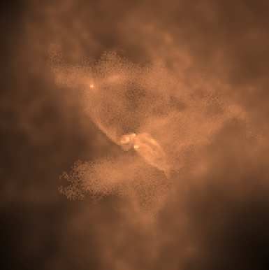
Publications of the Astronomical Society of Japan, (2021), Vol. 00, No. 0                                                           3

responding to the formation region for the stars with the                   This study is the first in a series of the SIRIUS
lowest mass in the simulations of Milky Way mass galaxies.              (SImulations Resolving IndividUal Stars) project, which
There are no computational resources that can compute                   seeks to understand the chemo-dynamical evolution of
such simulations. If we adopt the sink particle approach                star clusters and galaxies with high-resolution simulations.
to galaxy formation simulations with a mass resolution of               This project consists of three code papers: star formation
> 10 M⊙ , a large amount of gas (typically > 500 M⊙ ) is                model (this study), ASURA+BRIDGE code (Fujii et al.
∼                                               ∼
locked up in a sink particle. In the case of poor resolution,           2021b), and feedback (Fujii et al. 2021a) and subsequent
not all gas particles are going to form stars, resulting in             science papers. The purpose of this study is to construct
locking too much non-star-forming gas in a sink particle.               a star formation model for star-by-star simulations and
Kim & Ostriker (2017) have shown that the ISM properties                clarify the effects of parameters of the model in the simu-
such as vertical velocity dispersion and hot gas fraction do            lations. In this study, we perform a series of star cluster
not converge in simulations with the grid resolution larger             formation simulations from turbulent molecular clouds to
than 16 pc because supernovae are clustered in the large                test the newly developed models. We study the condition
sink particles. These consequences mean that we cannot                  to sample the IMF in this model and the influence of the
apply the sink particle approach to galaxy formation sim-               parameters in star-by-star simulations.
ulations.                                                                   This paper is organized as follows. The next section
   In almost all galaxy formation simulations, the simple               describes the implementation of the star formation models
stellar population (SSP) approximation, which considers a               for star-by-star simulations. Section 3 shows the code and
stellar component as a cluster of stars sharing the same                initial conditions. Section 4 systematically studies the ef-
age and metallicity with a given stellar initial mass func-             fects of parameters on the sampling of the assumed IMF
tion (IMF), is used to model star formation. With this                  in star clusters. Section 5 discusses the formation of an
approximation, once a gas particle satisfies a set of con-              ultra-faint dwarf galaxy (UFD). In section 6, we discuss
ditions imitating real star forming regions, (a part of) its            the applicability of our model. Section 7 summarizes the
mass converts into a collision-less star particle by following          main results.
Schmidt’s law (Schmidt 1959):
dρ∗    dρgas      ρgas
    =−       ≡ c∗      ,                                       (1)
 dt     dt        tdyn                                                  2 Star formation scheme
where ρ∗ and ρgas exhibit stellar and gas densities, respec-            2.1 Procedure for star formation
tively, tdyn is the local dynamical time, and c∗ is a dimen-
sionless parameter ranging from 0.01 − 0.1 (Katz 1992).                 The models of star formation developed for simulations
Although there are some variations in modeling star for-                with SSP approximation (e.g., Katz 1992; Okamoto et al.
mation and its conditions (e.g., Navarro & White 1993;                  2003; Stinson et al. 2006; Saitoh et al. 2008) must be mod-
Steinmetz & Mueller 1994; Stinson et al. 2006; Saitoh et al.            ified for star-by-star simulations of star clusters and galax-
2008; Hopkins et al. 2011), the star formation models used              ies. The intended mass resolution is mgas ≤ mmax, IMF in
in galaxy formation simulations are essentially the same.               this study. We also assumed that the stellar mass from the
    These star formation models cannot be easily applied to             adopted IMF was assigned to each star particle.
star-by-star simulations because of the breakdown of the                   In this section, we describe the procedure for the pro-
SSP approximation. Revaz et al. (2016) have shown that                  posed star formation model. The first step was to check the
the SSP approximation cannot correctly sample the IMF                   conditions for star formation. Gas particles became eligible
in the simulations of mass resolution of <       3
                                            ∼ 10 M⊙ . Since
                                                                        for star formation when they were conversing (∇ · v < 0) in
we have not yet understood what conditions derive IMFs,                 a higher density region than the threshold density (nth )
we need to rely on the stochastic sampling of IMFs (e.g.,               and in a colder region than the threshold temperature
Howard et al. 2014; Hu et al. 2017; Hu 2019). This case                 (Tth ). Gas particles that formed stars during the given
requires star particles with different masses. If the mass of           time interval ∆t were stochastically selected by the follow-
a star particle is larger than the mass of a gas particle, the          ing equation:
masses from surrounding gas particles must be accounted
                                                                             mgas                   ∆t
for. Moreover, the IMF should be sampled correctly in suf-              p=           1 − exp −c∗               ,                  (2)
                                                                             hm∗ i                 tdyn
ficiently large systems. However, there are no systematic
studies for modeling star-by-star simulations. It is neces-             where mgas , hm∗ i, c∗ , and tdyn were the mass of one gas
sary to confirm that the model can correctly sample the                 particle, the average value of stellar mass in the assumed
IMFs and compute properties of star clusters and galaxies.              IMF, the dimensionless star formation efficiency, and the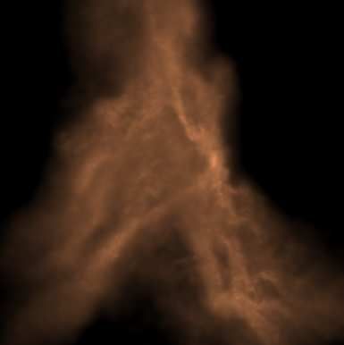
4 Publications of the Astronomical Society of Japan, (2021), Vol. 00, No. 0
local dynamical time, respectively.1 We set the dimen-
sionless star formation efficiency as 0.02 and 0.1 following
its observed constraints per free-fall time (Krumholz et al.
2019, and references therein).
We introduced the coefficient, mgas /hm∗ i. This expres-
sion was adopted to scale the number of newly formed stars
to the mass resolution. Note that the denominator of the
coefficient was not the mass of the star particle (m∗ ), which
was adopted in models of Okamoto et al. (2003); Stinson
et al. (2006); instead, it was the average stellar mass com-
puted from the adopted IMF (hm∗ i). This difference came
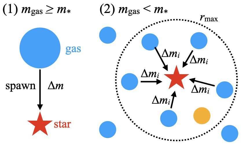
from the mass of each star particle. The masses of each star Fig. 1. Illustration of our star formation scheme. Gas particles that satisfied
particle in the SSP approximation were almost constant, all conditions of star formation were eliminated from the source of mass to
form a new star particle (yellow plot). The black-dashed circle represents the
whereas the masses were different among star particles in
maximum search radius (rmax , color online).
our case.
The second step was to compare the value of p to the
tained a mass of 5–10 m∗ (≡ minc ). We then adopted the
random number (R) from 0 to 1. If p > R, we assigned
maximum search radius (rmax ) to gather gas mass to form
stellar mass (m∗ ) from the minimum (mmin, IMF ) to the
stars and prevent an assemblage of this mass in an unre-
maximum (mmax, IMF ) mass of the IMF using the Chemical
alistically large region. If the required radius to assemble
Evolution Library (CELib, Saitoh 2017). The detailed im-
the gas mass in the region containing the mass of minc
plementation of CELib is described in section 2.2.
exceeded rmax , we forced the search radius to be rmax .
In the final step, gas particles that satisfied all con-
We estimated the required search radius (rth ) to form
ditions of star formation were converted into star parti-
a star with a mass m∗ by the following equation:
cles through one of two methods depending on whether
31
the mass of a gas particle (mgas ) was larger than m∗ or 3m∗
rth = , (4)
not. Figure 1 shows the schematic for converting gas par- 4πnH mH
ticles into a star particle. In the case of mgas ≥ m∗ , a where nH and mH were the number density and mass of hy-
gas particle was spawned to form a star particle (case 1 drogen, respectively. To form a star with a mass of 100 M⊙
in figure 1). The mass of the gas particle was reduced by in a region of nH = 1.2 × 105 cm−3 and nH = 1.2 × 107 cm−3 ,
∆m = mgas − m∗ . Positions and velocities of the par- the maximum search radius must be larger than 0.21pc and
ent gas particles are inherited to the newly formed stars. 0.04 pc, respectively. If the gas mass within rmax was less
When mgas > hm∗ i, mass resolution of the simulation was than 2 m∗ , we randomly re-assign the smaller stellar mass
not enough to explicitly sample all mass ranges of stars in for a star particle. If there were gas particles that satisfied
the IMFs. Several ways were proposed to assign proper- all conditions of star formation, they were excluded from
ties of stars to star particles (Colı́n et al. 2013; Hu et al. the mass transfer. Gas particles with temperature higher
2017; Hu 2019; Applebaum et al. 2020). Since all mod- than 103 K were also excluded to prevent assembling of
els in this study had mmin, IMF ≤ 1.5 M⊙ , lifetimes of un- mass from hot gas.
sampled stars were much longer than the total time of the We then converted the gas particle at the center of this
performed simulations. We did not put the effect of stellar region into a star particle. Positions (x∗,new ) and velocities
evolution of low mass stars in this study. (v∗,new ) of a newly star particles were re-assigned to ensure
If mgas < m∗ , a star particle was generated by assem- the momentum conservation. If the positions and velocities
bling masses of surrounding gas particles (case 2 in figure of the parent gas particle were xgas,p and vgas,p , x∗,new and
1). In this case, we first determined the region that con- v∗,new were reassigned as follows:
1
m∗ xgas,p + f ΣN
i=0 mgas,i xgas,,i
list
We can rewrite equation 2 as follows if c∗ ∆t/tdyn ≪ 1: x∗,new = N
, (5)
n o m∗ + f Σi=0
list
mgas,i
mgas ∆t
p= 1 − exp −c∗ . (3)
hm∗ i tdyn m∗ vgas,p + f ΣN
i=0 mgas,i vgas,,i
list
v∗,new = N
, (6)
This expression is harmonized to star formation’s probabilistic manner be- m∗ + f Σi=0
list
mgas,i
cause its range is from 0 to unity. In our numerical experiments, both
where xgas,i , vgas,i , mgas,i were positions, velocities,
expressions provided almost the same results, which indicated that the
condition c∗ ∆t/tdyn ≪ 1 was satisfied in our simulations. In this study, and masses of assembled gas particles, respectively.
we used equation 2. The amount of reduced gas mass was set as f ≡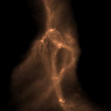
Publications of the Astronomical Society of Japan, (2021), Vol. 00, No. 0 5
(m∗ − mgas) /minc . t∗ ∝ m−3 ∗ ). Lifetimes of stars from 150 to 300 M⊙ were
Next, we reduced the masses of surrounding gas parti- taken from Schaerer (2002).
cles. The mass of gas particles after mass conversion was We adopted the IMF of Chabrier (2003) in the models,
(1−f )mgas to satisfy the mass conservation. After the star except for M40ks and M40kt. Recent observations of low
formation, gas particles with ten times less massive than mass stars suggested that the IMF in the low mass range
the average gas particle mass were merged to the nearest shows a flatter index of the power law than −1.35 (Kroupa
neighbor gas particle. When two particles were merged, 2001). The functional form of the adopted Chabrier IMF
the positions and velocities of merged particles were the is as follows:
centers of mass of two particles to ensure momentum con-
m ) 2
{log10 ( 0.079 }
servation. This scheme was introduced to prevent gas par-
exp − 2(0.69) 2 ,
dN
ticles that have significantly less massive than gas particles ∝ (0.1 M⊙ ≤ m ≤ 1 M⊙ ), (7)
in its neighborhood. d log10 m
m−1.3 ,
(1 M⊙ < m ≤ 100 M⊙ ),
2.2 Sampling of the IMF by CELib where m and N were the mass and the number of stars,
respectively. We also adopted the classical Salpeter IMF
We updated CELib to assign stellar masses to newly
(Salpeter 1955) from 0.1 to 100 M⊙ :
formed star particles. CELib first converted lifetimes to
a table numbered from 0 to 1 as weighted by the IMF (fig- dN
∝ m−1.35 , (8)
ure 2). It then assigned the stellar mass and the lifetime d log10 m
to the new star particle. and the IMF suggested from the simulation of the
Population III star formation (hereafter, we refer to this
IMF as Susa IMF; Susa et al. 2014). We defined the Susa
IMF from 0.7 to 300 M⊙ as follows:
1.0
(
m
2 )
dN log10 22.0
∝ exp − . (9)
d log10 m 2(0.5)2
0.8
Cumlative number of stars
This IMF was characterized by a large fraction of massive
stars.
0.6 Figure 3 shows the mass function stochastically gener-
ated by CELib using 106 samples. We generated 106 ran-
0.4 dom numbers from 0 to 1 by CELib and then assigned stel-
lar mass following the lifetime table weighted by the IMF.
0.2 Note that the IMF was generated not by N -body/SPH
simulations but by only using CELib. As shown in this
figure, CELib can sample the assumed IMFs. Deviations
0.0
seen in higher mass stars were caused by the small number
108 1010 1012 of samples.
log10[t* (yr)]
Fig. 2. Cumulative number normalized from 0 to 1 of stars with solar metal- 3 Simulations
licity as a function of the lifetime (t∗ ).
3.1 Code
Stellar lifetimes from lifetime tables were interpolated We adopted an N -body/SPH simulation code, ASURA
via polynomial function fitted using the least-squares fit- (Saitoh et al. 2008, 2009). Gravity was computed using
ting method (Saitoh 2017). We used the stellar lifetime the tree method (Barnes & Hut 1986) with the tolerance
table from Portinari et al. (1998) for 0.6 to 100 M⊙ . This parameter θ = 0.5. Because star clusters were collisional
lifetime represented the sum of the timescales of hydrogen- systems, these objects should be treated as direct N -body
and helium-burning computed in the Padova stellar evo- (e.g., Fujii et al. 2007; Hubber et al. 2013a; Wall et al. 2019)
lution library (Bressan et al. 1993; Fagotto et al. 1994a, to force the accuracy to a sufficiently high level. We did
1994b). For lifetimes (t∗ ) of stars with less than 0.6 M⊙ , not, however, apply a direct N -body computation in this
we extrapolated the lifetime table using the stellar mass- study; this was to avoid increasing uncertain parameters.
luminosity (L) relationship (L ∝ m4∗ , t∗ ∝ m∗ L−1 , i.e., Our next paper will show the implementation of the direct
6                                                                         Publications of the Astronomical Society of Japan, (2021), Vol. 00, No. 0

Fig. 3. The IMFs generated by CELib (red-solid curve). The blue-dashed curve represents (a) Chabrier IMF, (b) Salpeter IMF, and (c) Susa IMF (color online).

N -body and its effects on the properties of star clusters                      sonic turbulent motion of gas was modeled as a divergence-
(Fujii et al. 2021b).                                                           free random Gaussian velocity field proportional to the
    Hydrodynamics in ASURA were computed with the                               wave number of velocity perturbations with a power law
density-independent SPH method (Saitoh & Makino                                 index of −4 (Ostriker et al. 2001). The initial total gas
2013). An artificial viscosity was introduced to handle                         masses of clouds were set as 1 × 10³ M⊙ (models B03)
shocks. We adopted a variable viscosity model proposed                          and 4 × 10⁴ M⊙ (models M40k). The mass resolution of
by Morris & Monaghan (1997) with a slight modification                          model B03h was the same as the model adopted in Bonnell
of Rosswog (2009). We implemented a timestep limiter                            et al. (2003). The radii of the clouds were 0.5 pc and
for the supernova shocked region (Saitoh & Makino 2009)                         10.0 pc for models B03 and M40k, respectively. The free-
and a Fully Asynchronous Split Time-Integrator (FAST,                           fall times for the clouds of B03 and M40k were 0.19 and
Saitoh & Makino 2010) to accelerate the computation.                            0.83 Myr, respectively. We set the gravitational softening
We applied the cooling and heating function from 10 to                          length and the threshold density for star formation follow-
109 K, as generated by Cloudy ver.13.05 (Ferland et al.                         ing the Jeans length, assuming that the Jeans mass was
1998, 2013, 2017). At the end of the lifetime, stars with                       resolved by 100 gas particles and the temperature was 20
13 to 40 M⊙ exploded as core-collapse supernovae. We as-                        K. For models with mass resolutions of 0.001, 0.002, 0.01,
sumed that each supernova distributes thermal energy of                         0.02, and 0.1 M⊙ , the softening lengths corresponded to
1051 erg and elements to surrounding gas particles with the                     3.2 × 10² , 6.5 × 10² , 3.2 × 10³ , 6.5 × 10³ , and 3.2 × 10⁴ au,
yield of Nomoto et al. (2013). We did not implement other                       respectively. We set the metallicity as Z = 0.013 (Asplund
types of nucleosynthetic events. Metal diffusion was also                       et al. 2009). Table 1 lists the models adopted in this study.
computed based on the turbulence-motivated model (Shen
et al. 2010; Saitoh 2017; Hirai & Saitoh 2017). We set the
scaling factor for metal diffusion as 0.01 following Hirai                      3.2.2 Cosmological zoom-in simulations of ultra-
& Saitoh (2017). For cosmological zoom-in simulations,                                faint dwarf galaxies
we also implemented the effects of ultra-violet background
                                                                                We performed a cosmological zoom-in simulation of an
field (Haardt & Madau 2012) and self-shielding (Rahmati
                                                                                UFD. The initial condition was generated by music (Hahn
et al. 2013).
                                                                                & Abel 2011). A pre-flight N -body simulation was per-
                                                                                formed using Gadget-2 (Springel 2005) with a box size of
3.2 Initial conditions                                                          (4 Mpch−1 )3 . A halo for a zoom-in simulation was selected
3.2.1 Star clusters from turbulent molecular                                    using AMIGA halo finder (Gill et al. 2004; Knollmann
        clouds                                                                  & Knebe 2009). We selected a halo with a mass of
We adopted the turbulence-molecular cloud model                                 4.9 ×10⁸ M⊙ at the redshift z = 3. We confirmed that there
(Bonnell et al. 2003; Fujii 2015; Fujii & Portegies                             were no halos over 1012 M⊙ within 1Mpc from the zoomed-
Zwart 2015, 2016) using initial conditions generated by                         in halo.
the Astronomical Multipurpose Software Environment                                 A zoom-in hydrodynamic simulation was performed us-
(AMUSE, Portegies Zwart et al. 2009, 2013; Pelupessy                            ing ASURA. The total number of particles in the zoomed-
et al. 2013; Portegies Zwart & McMillan 2018). The super-                       in initial condition was 3.8× 10⁷ . Masses of a dark mat-
Publications of the Astronomical Society of Japan, (2021), Vol. 00, No. 0 7
Table 1. List of models.∗
Name Mtot (M⊙ ) rt (pc) Ng mg (M⊙ ) ǫg (au) nth (cm−3 ) rmax (pc) c∗ IMFs
B03vh 1 × 10³ 0.5 1× 10⁶ 0.001 3.2 × 10² 1.2 × 10⁹ 0.2 0.02 Chabrier (2003)
B03h 1 × 10³ 0.5 5× 10⁵ 0.002 6.5 × 10² 3.0 × 10⁸ 0.2 0.02 Chabrier (2003)
B03m 1 × 10³ 0.5 1× 10⁵ 0.01 3.2 × 10³ 1.2 × 10⁷ 0.2 0.02 Chabrier (2003)
B03l 1 × 10³ 0.5 5× 10⁴ 0.02 6.5 × 10³ 3.0 × 10⁶ 0.2 0.02 Chabrier (2003)
B03vl 1 × 10³ 0.5 1× 10⁴ 0.1 3.2 × 10⁴ 1.2 × 10⁵ 0.2 0.02 Chabrier (2003)
B03e 1 × 10³ 0.5 1× 10⁵ 0.01 3.2 × 10⁴ 1.2 × 10⁵ 0.2 0.02 Chabrier (2003)
B03n 1 × 10³ 0.5 1× 10⁵ 0.01 3.2 × 10³ 1.2 × 10⁵ 0.2 0.02 Chabrier (2003)
B03c 1 × 10³ 0.5 1× 10⁵ 0.01 3.2 × 10³ 1.2 × 10⁷ 0.2 0.2 Chabrier (2003)
B03sr 1 × 10³ 0.5 1× 10⁵ 0.01 3.2 × 10³ 1.2 × 10⁷ 0.02 0.02 Chabrier (2003)
B03lr 1 × 10³ 0.5 1× 10⁵ 0.01 3.2 × 10³ 1.2 × 10⁷ 2.0 0.02 Chabrier (2003)
M40km 4 × 10⁴ 10.0 4× 10⁶ 0.01 3.2 × 10³ 1.2 × 10⁷ 0.2 0.02 Chabrier (2003)
M40kl 4 × 10⁴ 10.0 4× 10⁵ 0.1 3.2 × 10⁴ 1.2 × 10⁵ 0.2 0.02 Chabrier (2003)
M40ke 4 × 10⁴ 10.0 4× 10⁶ 0.01 3.2 × 10⁴ 1.2 × 10⁵ 0.2 0.02 Chabrier (2003)
M40ksr 4 × 10⁴ 10.0 4× 10⁵ 0.1 3.2 × 10⁴ 1.2 × 10⁵ 0.02 0.02 Chabrier (2003)
M40klr 4 × 10⁴ 10.0 4× 10⁵ 0.1 3.2 × 10⁴ 1.2 × 10⁵ 2.0 0.02 Chabrier (2003)
M40ks 4 × 10⁴ 10.0 4× 10⁵ 0.1 3.2 × 10⁴ 1.2 × 10⁵ 0.2 0.02 Salpeter (1955)
M40kt 4 × 10⁴ 10.0 4× 10⁵ 0.1 3.2 × 10⁴ 1.2 × 10⁵ 0.5 0.02 Susa et al. (2014)
UFD 1 × 10⁷ 770 2× 10⁷ 18.4 1.9 × 10⁶ 1.0 × 10² 2.2 0.02 Chabrier (2003)
∗
From left to right, the columns show the names of the models, the initial total gas mass (Mtot ), the initial truncation radius (rt ), the
initial number of gas particles (Ng ), the mass of one gas particle (mg ), the gravitational softening length (ǫg ), the threshold density for
star formation (nth ), the maximum search radius (rmax ), the dimensionless star formation efficiency parameter (c∗ ), and adopted IMFs.
ter particle and a gas particle were 99.0 M⊙ and 18.5 M⊙ , 4c).
respectively. To avoid making stars with masses largely
different from gas particles, we set the Chabrier IMF from Figure 5 shows gas density probability distribution
1.5 M⊙ to 100 M⊙ . This assumption let average star par- function (PDF) in model B03h. This gas density
ticle mass 4.7 M⊙ , corresponding to 0.25 times the mass PDF can be well fitted with a log-normal PDF. The
of gas particles. This value led to a good balance between mean density (hlog10 nH i) and the standard deviation
time resolution and CPU time (Springel & Hernquist 2003; (σ) are hlog10 nH i = 4.89, σ = 0.86 at 0.15 Myr and
Revaz & Jablonka 2012). We set the gravitational soft- hlog10 nH i = 3.38, σ = 1.06 at 0.45 Myr. Decrease of the
ening lengths of dark matter particles as 19.8 pc follow- mean density is owing to the star formation. At 0.45 Myr,
ing (Hopkins et al. 2018b). The softening lengths of gas the cloud develops the power-law tail in a high-density re-
and star particles were set to contain 100 gas particles in gion (see section 6.1 for the discussion).
the threshold density. In this simulation, this value corre-
sponded to 9.1 pc.
4.1.1 Mass resolution
4 Star cluster formation Figure 6 shows the total stellar mass as a function of time
in models of different mass resolutions. The total stellar
4.1 Formation of star clusters from the turbulent
masses in models B03vh, B03h, B03m, and B03l are 551,
molecular clouds with 103 M⊙
556, 452, and 320 M⊙ , respectively, at 0.45 Myr. These
The turbulent motion of the gas induced the evolution of masses are similar to those in Bonnell et al. (2003, see
the molecular cloud. Figure 4 shows snapshots of gas and section 6.1). As shown in section 3.2, the Jeans lengths
stellar density distributions in model B03h. We placed the in the star forming regions in these models are less than
cloud with the random Gaussian velocity field as described 6.5 × 10³ au (= 3.2 × 10⁻² pc). These sizes are significantly
in section 3.2 (figure 4a). Supersonic turbulent motion in smaller than that of the system (= 5.0 × 10⁻¹ pc), allow-
this model produced shocks leading to the formation of ing them to detail the star formation process. They can
filamentary structures. Shocks also expelled the kinetic therefore convert over 30% of gas to stars. However, model
energy of the gas. This effect locally reduced the support B03vl only has a total stellar mass of 14 M⊙ at 0.45 Myr.
of turbulence. Once high density regions in the filament Because the Jeans length 3.2 × 10⁴ au (= 1.6 × 10⁻¹ pc)
self-gravitate, they collapse and can form stars (figure 4b). is a similar size as that of the system, this model cannot
After the star formation begins, gases are consumed (figure emulate the star formation process correctly.8 Publications of the Astronomical Society of Japan, (2021), Vol. 00, No. 0
0.4 (a) 0.00 Myr 0.4 (b) 0.25 Myr 0.4 (c) 0.45 Myr
y (pc)
0.2 0.2 0.2
y (pc)
y (pc)
0.0 0.0 0.0
−0.2 −0.2 −0.2
−0.4 −0.4 −0.4
−0.4 −0.2 0.0 0.2 0.4 −0.4 −0.2 0.0 0.2 0.4 −0.4 −0.2 0.0 0.2 0.4
x (pc) x (pc) x (pc)
Fig. 4. Gas column density and stellar distributions in model B03h. Panels (a), (b), and (c) represent snapshots at 0.00, 0.25, and 0.45 Myr from the beginning
of the simulation, respectively. The color gradation shows the logarithm of the column density from 1021 cm−2 (black) to 1025 cm−2 (yellow). White dots
depict stars. Larger sizes of dots represent more massive stars (color online).
10−1
102
10−2
Stellar mass (M⊙)
101
PM
B03vh
10−3 0 B03h
10
B03m
0.15 Myr B03l
0.45 Myr 10−1
B03vl
10−4 −1
10 101 103 105 107 0.0 0.1 0.2 0.3 0.4
log10(nH(cm−3)) Time (Myr)
Fig. 5. The density distribution of gas in model B03h at 0.15 Myr (the orange- Fig. 6. Total stellar mass as a function of time from the beginning of the
solid curve) and 0.45 Myr (the blue-solid curve) from the beginning of the simulation (the solid blue curve: B03vh, the dashed orange curve: B03h, the
simulation. Orange- and blue-dashed curves represent the best-fit log- dash-dotted green curve: B03m, the dotted red curve: B03l, and the solid
normal curves at 0.15 Myr and 0.45 Myr, respectively (color online). purple curve: B03vl; color online). The dotted brown line depicts the total
stellar mass (415 M⊙ ) at 0.45 Myr in the model computed in Bonnell et al.
(2003).
4.1.2 Gravitational softening length and threshold
density for star formation
We have varied the gravitational softening length and ilar level as model B03vl. This result means that resolving
threshold density for star formation to clarify the parame- the self-gravitating clumps is one of the keys for forming
ters that show the largest impacts on the total stellar mass stars in these models. Models B03vl and B03e do not have
of the system. Both parameters are related to the resolu- a sufficiently high resolution to resolve star-forming clumps
tion of the simulation. The effect of gravitational soften- in the molecular cloud.
ing is evident in figure 7a. Model B03e adopts the same Lack of sufficient spatial resolution prevents resolving
parameters of gravitational softening length and threshold high-density gas. Figure 8 shows gas density PDFs in mod-
density for star formation as model B03vl (ǫg = 3.2 × 10⁴ au els B03m and B03e. As shown in this figure, model B03e
and nth = 1.2 × 105 cm−3 ) but has the same mass resolution lacks gas with > 6 −3
∼ 10 cm , which cannot be resolved in this
as model B03m (mg = 0.01 M⊙ ). As shown in this figure, model. These results mean that if the gravitational soften-
the star formation in model B03e is suppressed at the sim- ing length is excessively large compared to the size of thePublications of the Astronomical Society of Japan, (2021), Vol. 00, No. 0 9
(a) (b) (c)
2 2 2
10 10 10
Stellar mass (M⊙)
Stellar mass (M⊙)
Stellar mass (M⊙)
101 101 101
100 100 100
B03m
B03e B03m B03m
−1 B03vl −1 B03n −1 B03c
10 10 10
0.0 0.1 0.2 0.3 0.4 0.0 0.1 0.2 0.3 0.4 0.0 0.1 0.2 0.3 0.4
Time (Myr) Time (Myr) Time (Myr)
Fig. 7. Similar to figure 6, but for models (a) B03m (solid blue curve), B03e (dashed orange curve), B03vl (dash-dotted green curve), (b) B03m (solid blue
curve), B03n (dashed orange curve), (c) B03m (solid blue curve), and B03c (dashed orange curve, color online).
system, the star formation cannot be computed correctly. are similar, owing to the limited initial total gas mass of
the cloud (= 1000 M⊙ ).
Model B03n begins star formation earlier than that of
model B03m (figure 7b). The conditions of star formation
10−1 are more easily satisfied in models with a lower value of
B03m nth . These results suggest that the choice of nth does not
B03e
considerably affect the formation of stars in this model.
10−2 4.1.3 Star formation efficiency
The value of c∗ does not strongly affect the total stellar
PM
mass of the system. Model B03c (c∗ = 0.1) has a stellar
mass of 554 M⊙ . This mass is only 1.2 times larger stellar
10−3 mass than that of model B03m (452 M⊙ , see figure 7c),
whereas model B03c has a value of c∗ that is five times
larger than that of model B03m. The threshold density for
star formation (nth = 1.2 × 107 cm−3 ) is 2 dex larger than
10−4 −1 the mean density of the cloud (∼ 105 cm−3 ). Because we
10 101 103 105
have adopted the Schmidt law (equation 1), the timescale
log10(nH(cm−3))
of the star formation is short enough to diminish the effect
of c∗ in this case. Therefore, the value of c∗ does not
Fig. 8. Similar to figure 5, but for models B03m (blue-solid curve) and B03e
substantially affect the total stellar mass of the system.
(orange-dashed curve, color online).
The value of the threshold density for star formation 4.1.4 Maximum search radius
does not substantially affect the total stellar mass of the The maximum search radius does not affect the time
system. Figure 7b compares the time evolution of the evolution of the total stellar mass. Figure 9a shows
stellar masses in models B03n (nth = 1.2 × 105 cm−3 ) and the total stellar mass as a function of time in models
B03m (nth = 1.2 × 107 cm−3 ). In model B03n, the stellar B03sr (rmax = 0.02 pc), B03m (rmax = 0.2 pc), and B03lr
mass at 0.45 Myr is 423 M⊙ . This value is similar to that (rmax = 2.0 pc). As shown in this figure, there is no signif-
of model B03m (452 M⊙ ). Regardless of the value of nth , icant difference among the models.
most of the stars are formed in a region with a significantly Regardless of the value of the maximum search radius,
higher density than the threshold for star formation. The the assumed IMF for stars with a mass lower than 10 M⊙
average star formation density at 0.25 Myr in models B03m is reproduced in model B03. Figure 9b represents the stel-
and B03n are 1.2 × 108 cm−3 and 4.9 × 107 cm−3 , respec- lar mass functions computed in models B03sr, B03m, and
tively. The total stellar masses at 0.45 Myr in both models B03lr. For stars larger than 1 M⊙ , the mass function fol-10 Publications of the Astronomical Society of Japan, (2021), Vol. 00, No. 0
102
B03sr 100 B03sr
(a) (b) (c)
B03m B03m
102 B03lr B03lr
Chabrier IMF
Stellar mass (M⊙)
Cumulative mass
Number of stars
101 101
100
B03sr 10−1
B03m
B03lr
10−1 100
0.0 0.1 0.2 0.3 0.4 10−1 100 101 102 10−1 100 101 102
Time (Myr) Stellar mass (M⊙) Stellar mass (M⊙)
Fig. 9. The effect of the maximum search radius in models B03sr (rmax = 0.02 pc, solid blue curves), B03m (rmax = 0.2 pc, dashed orange curves), and B03lr
(rmax = 2.0 pc, dash-dotted green curves). (a) Total stellar mass as a function of time, (b) the number of stars as a function of the mass of each star particle,
and (c) cumulative mass functions. Panels (b) and (c) are plotted at 0.45 Myr from the beginning of the simulation. The red dotted curve in panel (b) represents
the Chabrier IMF (color online).
lows the power-law distribution with an index of −1.3. The as a function of time in models B03m, B03m1, B03m2,
flattening shape in lower mass stars is caused by adopting B03m3, and B03m4. These models adopt the same pa-
the log-normal distribution in the Chabrier IMF. rameters except for random number seeds of the initial
Figure 9c denotes the cumulative mass of stars as a conditions. Owing to the randomness of the turbulent ve-
function of the stellar mass. According to this figure, the locity field, the onset of star formation varies from 0.19
cumulative masses of models B03m and B03lr are the same. to 0.25 Myr. The final stellar mass is also different among
These models adopt the same parameters, except for the the models. The lowest stellar mass at 0.45 Myr is 141 M⊙
maximum search radius. The required search radius to whereas the highest is 478 M⊙ .
form a star with 100 M⊙ in these models is rth = 0.04 pc
(equation 4). Models B03m and B03lr have larger values
of rmax than rth . This result implies that the maximum
search radius does not affect the stellar mass function as
far as its size is larger than that expected from the density B03m
of the star-forming region. B03m1
102 B03m2
The formation of the most massive stars appears to be
B03m3
Stellar mass (M⊙)
suppressed in model B03sr. However, it is difficult to eval- B03m4
uate the effects of the maximum search radius on the for-
mation of massive stars in this model. Because the mass
101
of the cloud has only 1000 M⊙ and the typical conversion
fraction of gas to stars is ∼ 0.4, a few massive stars are
formed in these models. In section 4.2, we discuss the ef-
100
fects of using a maximum search radius with more massive
clouds.
10−1
0.0 0.1 0.2 0.3 0.4
4.1.5 Run-to-run variations Time (Myr)
When we set the turbulent velocity field for the initial con-
ditions, we used a random number. The randomness in the Fig. 10. Similar to figure 6, but for models with different random number
turbulence affects the shape of collapsing molecular clouds seeds of initial conditions. The different colors represent models with dif-
and the star clusters forming within them. To clarify run- ferent random number seeds (color online).
to-run variations, we performed four additional runs for
model B03m, but with different random seeds for the tur- Molecular clouds of less than 1000 M⊙ do not have
bulent velocity field. Figure 10 shows the total stellar mass enough mass to adequately sample the IMF from 0.1 toPublications of the Astronomical Society of Japan, (2021), Vol. 00, No. 0 11
100 M⊙ . The fraction of massive stars is only a small per- lier phases than in model M40kl. The former model can
centage in all stars. The random number seed for the ini- resolve turbulent motions of gas more accurately than the
tial conditions and star formation affect the formation of latter. The chaotic nature of turbulence motion induces a
massive stars in these small clouds. Figure 11 compares high-density region locally. Models with a higher mass res-
cumulative mass function in models with different random olution have more chances to form a star-forming region,
number seeds. Even if we assume the same initial gas mass, thus forming stars in an earlier phase.
the masses of the most massive stars formed in these mod- On the other hand, models B03 have a considerably
els vary from 23.5 M⊙ to 91.0 M⊙ . Thus, the formation of high density (the free-fall time of 0.19 Myr) and compact
massive stars in small molecular clouds is highly stochas- clouds. In this model, the conditions for star formation can
tic. This model is therefore not suitable for evaluating the be easily satisfied. Therefore, the onset of star formation
effects of the value of rmax on the sampling of IMFs. in models B03 weakly depends on the mass resolution.
4.2.2 Gravitational softening length
The choice of gravitational softening length in M40k does
not largely affect the evolution of the stellar mass in the
100
adopted range of ǫg , but the effect is similar to the models
B03. M40ke adopts the same gravitational softening length
as in M40kl (ǫg = 3.2 × 10⁴ au), but the initial number of
gas particles is the same as that in M40km (Ng = 4.0 ×10⁶ ).
Cumulative mass
We have shown that star formation is significantly sup-
pressed by increasing the gravitational softening length in
B03. In contrast, the star formation is not suppressed in
B03m
M40ke (the green dash-dotted curve in figure 13). This
B03m1
B03m2 difference is caused by the size of the clouds. B03 has a
10−1 B03m3 radius of 0.5 pc, which is comparable to the size of the soft-
B03m4 ening length of B03l. However, the softening size is much
smaller than the radius of M40k (rt = 10pc). Thanks to the
10−1 100 101 102 large radius compared to the adopted gravitational soft-
Stellar mass (M⊙)
ening length, M40kl can form stars even if the softening
length is the same as B03l, which excessively suppresses
Fig. 11. Similar to figure 9c, but for models with a different random number star formation.
seed. Different colors represent models with different random number seeds
(color online).
4.2.3 Maximum search radius
The maximum search radius does not largely affect the
evolution of the total stellar mass also in M40k. Figure
4.2 Formation of star clusters from the turbulent 14a represents the total stellar mass as a function of time
molecular clouds with 4 × 10⁴ M⊙ in models M40ksr (rmax = 0.02 pc), M40kl (rmax = 0.2 pc),
The star formation in a larger cloud similarly behaves with and M40klr (rmax = 2.0 pc). As shown in this figure, the
that of models B03. Figure 12 shows snapshots of gas and time evolution of the total stellar mass is the same in M40kl
stellar density distributions in model M40kl. The initial and M40klr. However, the total stellar mass in M40ksr is
condition (figure 12a) and the afterward evolution (figure lower than the other models. This result is owed to the
12b) are induced with the same mechanism with models formation of massive stars being suppressed in this model.
B03 (see section 4.1). This cloud makes several star clus- Figures 14b and 14c show the stellar mass functions
ters because of the large cloud’s mass (figure 12c). computed in M40ksr, M40kl, and M40klr. The cumulative
functions in M40kl and M40klr are overlap. Thus, choosing
4.2.1 Mass resolution a maximum search radius larger than rth does not affect
In this subsection, we describe the formation of star clus- the shape of the stellar mass function.
ters in a cloud with an initial gas mass of 4 × 10⁴ M⊙ . Setting an exceedingly small search radius prevents
Figure 13 shows the time evolution of stellar mass in mod- forming massive stars. Figure 14c clearly shows the lack of
els M40km and M40kl. Unlike model B03 (figure 6), the massive stars in M40ksr. The lack of massive stars in this
onset of star formation in model M40km is shifted to ear- model produces a larger number of low mass stars than12 Publications of the Astronomical Society of Japan, (2021), Vol. 00, No. 0
(a) 0.00 Myr (b) 2.30 Myr (c) 3.70 Myr
y (pc) 5 5 5
y (pc)
y (pc)
0 0 0
−5 −5 −5
−10−10 −5 0 5 10 −10−10 −5 0 5 10 −10−10 −5 0 5 10
x (pc) x (pc) x (pc)
Fig. 12. Similar to figure 4, but for model M40kl. Panels (a), (b), and (c) represent snapshots at 0.00, 2.30, and 3.70 Myr from the beginning of the simulation,
respectively (color online).
that models with a maximum radius smaller than the es-
timated search radius (equation 4) tend to underestimate
the fraction of massive stars.
Models with the appropriate size of a maximum search
104 radius can sample IMFs with a different shape. Figures
15 and 16 show stellar mass functions computed in models
103 with different IMFs. As shown in this figure, all models
Stellar mass (M⊙)
can fully sample the IMFs. Even if we assume Susa IMF, it
is possible to create stars with a stellar mass of ≈ 300 M⊙ .
102 The required maximum search radius to form stars with
300 M⊙ in a region of 1.2 × 105 cm−3 is 0.29 pc. In M40kt,
101 M40km
we set rmax = 0.5 pc. Thus, it is possible to fully sample
any form of IMFs if a sufficiently large search radius is
M40kl chosen.
100 M40ke The maximum search radius should be adjusted de-
0 2 4 6 pending on the threshold density of star formation (nth ).
Time (Myr) If nth = 104 cm−3 is chosen, rmax > 0.48 pc must be set to
allow a correct sampling of stars with 100 M⊙ . However,
Fig. 13. Similar to figure 6, but for models M40km (solid blue curve), M40kl if nth = 107 cm−3 is adopted, the required value of rmax is
(dashed orange curve), and M40ke (dash-dotted green curve, color online). only 0.05 pc. In summary, it is necessary to set a maxi-
mum search radius larger than the value estimated from
the threshold density for star formation to correctly sample
those of other models. The most massive star formed in
the assumed IMF.
M40ksr is 23.9 M⊙ , while M40kl and M40klr form stars
with 94.7 M⊙ and 100.0 M⊙ , respectively.
Notably, massive stars can be formed in sufficiently high 5 Dwarf galaxy formation
density regions even if a small search radius is chosen. In this section, we show that our star formation model
However, most stars tend to form slightly above the thresh- can be applied to galaxy formation simulations. Figure
old density for star formation (1.2 ×105 cm−3 in this case). 17 shows dark matter and stellar distribution of the sim-
This case does not improve the sampling of the IMF in ulated UFD. As shown in this figure, stars are formed at
models with a small maximum search radius. the center of the dark matter halo. The star formation
The choice of the maximum search radius affects the was quenched at the redshift z = 8.7 because the super-
number of massive stars. The expected number of massive nova feedback blow the gas away from the halo. At this
stars (10–100 M⊙ ) from the Chabrier IMF is ≈ 50 in a star redshift, total stellar and halo masses of this galaxy are
cluster with 5000 stars. In M40kl and M40ksr, there are 1.36 ×10³ M⊙ and 7.46 ×10⁶ M⊙ , respectively. The stellar
43 and 41 massive stars, respectively. On the other hand, mass-halo mass ratio is therefore 1.83 ×10⁻⁴ , meaning that
M40klr has only 13 massive stars. This result indicates this galaxy is highly dark matter dominated. This resultPublications of the Astronomical Society of Japan, (2021), Vol. 00, No. 0 13
103 100
(a) (b) M40ksr (c) M40ksr
104 M40kl M40kl
M40klr M40klr
Chabrier IMF
103 102
Stellar mass (M⊙)
Cumulative mass
Number of stars
102
101 10−1
101 M40ksr
M40kl
100 M40klr
100 −1
0 1 2 3 4 5 6 10 100 101 102 10−1 100 101 102
Time (Myr) Stellar mass (M⊙) Stellar mass (M⊙)
Fig. 14. Similar to figure 9, but for models M40ksr (solid blue curve), M40kl (dashed orange curve), and M40klr (dash-dotted green curve). Panels (b) and (c)
are plotted at the time when the total stellar mass reaches 4000 M⊙ (3.8 Myr for M40ksr and 3.7 Myr for M40kl and M40klr, color online).
M40ks 100
M40kl
103 M40kt
Salpeter IMF
Chabrier IMF
Cumulative mass
Number of stars
102 Susa IMF
M40ks
−1 M40kl
10 M40kt
101
Salpeter IMF
Chabrier IMF
Susa IMF
100 −1
10 100 101 102 10−1 100 101 102
Stellar mass (M⊙) Stellar mass (M⊙)
Fig. 15. Similar to figure 9b, but for models adopting different IMFs. The solid Fig. 16. Similar to figure 9c, but for models adopting different IMFs. The solid
blue, dashed orange, and dotted green curves represent M40ks (Salpeter blue, dashed orange, and dotted green curves represent M40ks (Salpeter
IMF), M40kl (Chabrier IMF), and M40kt (Susa IMF) at 6.0 Myr, respectively IMF) at 3.7 Myr, M40kl (Chabrier IMF) at 3.7 Myr, and M40kt (Susa IMF) at
(color online). 6.0 Myr, respectively(color online).
is consistent with the extrapolation from the abundance- the Chabrier IMF. The star with 40 M⊙ has already ex-
matching results, predicting the stellar mass of less than ploded as supernovae at the time of this snapshot. The
103 M⊙ in a halo with ∼ 107 M⊙ (Read et al. 2017). The lack of stars more massive than 40 M⊙ is owing to the
half-mass radius and velocity dispersion of this UFD are small total stellar mass (1.36 × 10³ M⊙ ). Models B03 (fig-
51 pc and 2.0 km s−1 . These values are consistent with the ure 9) also lack stars with the high-mass end of the IMF.
typical value of UFD around the Milky Way (Simon 2019). This result comes from the assumption that we restrict the
gas mass within rmax to be larger than 2 m∗ (see section
Expected stellar mass function is reproduced in this 6.3). The cut-off in the stellar mass function at the lowest
simulation. Figure 18 shows masses of star particles formed mass end is due to the lack of mass resolution. Since the
in this model. As shown in this figure, the slope of the stel- initial gas particle mass is 18.5 M⊙ in this simulation, we
lar mass function from 1.5 M⊙ to 40 M⊙ is consistent with set the minimum star particle mass to be 1.5 M⊙ in order14 Publications of the Astronomical Society of Japan, (2021), Vol. 00, No. 0
Chabrier IMF
102
Number of stars
101
100
100 101 102
Stellar mass (M⊙)
Fig. 17. Spatial distribution of dark mater and stars in the simulated UFD Fig. 18. Similar to figure 9b, but for the simulated UFD at z = 8.7. Plotted
at z = 8.7. The color scale represents the log-scale surface density of dark stellar mass is the initial stellar mass. The most massive star in this model
matter in each grid from 10−0.9 M⊙ pc−2 (black) to 102.3 M⊙ pc−2 (white). (40 M⊙ ) has already exploded as supernovae at the time of this snapshot.
Red circles show stars. More massive stars are drawn with larger plots (color Blue-solid and orange-dashed lines show the result of model UFD and the
online). expected number of stars from the Chabrier IMF, respectively (color online).
not to overproduce stars. Note that if we have to treat
feedback from low mass stars, we need to make compound
star particles (Hu et al. 2017; Applebaum et al. 2020). formation.
Our scheme satisfies the Kennicutt-Schmidt relation. It
is well know that the surface gas density and star formation
rates are expressed with
ΣSFR = AΣN
gas , (10)
−2.0 Kennic tt (1998)
where A and N are the constants (Schmidt 1959; Kennicutt Teich et al. (2016)
1989, 1998). Kennicutt (1998) has shown that the value of This st dy
−2.5
log[ΣSFR (M⊙ yr−⊙ kpc−2)]
the power-law index is N = 1.4 ± 0.15. Recent surveys have
found that this relation continues to dwarf galaxies (Teich
et al. 2016). Star formation models for galaxy formation
therefore needs to satisfy this relation.
−3.0
Figure 19 shows the surface density of star forma-
tion rates and gas in our simulation and observations. −3.5
In this simulation, we derive the surface density of gas
within 100 pc from the center of the galaxy (Σgas =
10−0.31 M⊙ pc−2 ) and star formation rates averaged in 100 −4.0
Myr (ΣSFR = 10−3.66 M⊙ yr−1 kpc−2 ). These values are
0.0 0.5 1.0
consistent with the Kennicutt-Schmidt relation. This re-
log[Σgas (M⊙ pc−2)]
sult is also consistent with the value in simulations of dwarf
galaxies, which adopts the star formation model similar to
this study (Gutcke et al. 2021). Since we computed the
Fig. 19. The Kennicutt-Schmidt relation (color online). The orange square
UFDs, both Σgas and ΣSFR are located in the lowest val- and blue filled-circles represent model UFD and observations by Teich et al.
ues. As we assume the local Schmidt law in this simulation (2016), respectively. Green line shows the fitted function in Kennicutt (1998).
(equation 1), we can confirm that it is possible to adopt
this star formation scheme to the simulations of galaxyPublications of the Astronomical Society of Japan, (2021), Vol. 00, No. 0 15
6 Discussion density for star formation. In model B03h, we assume
nth = 3.0 × 108 cm−3 (table 1) while the threshold den-
6.1 Comparison with other methods
sity corresponds to ∼ 1.5 × 104 cm−3 in model Σ-M5E4-
In this subsection, we compare results computed in pre- R15. In fact, model B03n (nth = 1.2 × 105 cm−3 ) starts
vious studies with different methods. We firstly discuss star formation ∼ 0.15 Myr earlier compared to model
the gas density PDF presented in figure 5. The shape B03m (nth = 1.2 × 107 cm−3 , figure 7b).
of the gas density PDF characterizes the evolution of the Early phases of the time evolution of stellar mass are dif-
gas (Vazquez-Semadeni 1994). Simulations of molecular ferent between models B03h and Σ-M5E4-R15. Raskutti
clouds (e.g., Ostriker et al. 2001; Vázquez-Semadeni & et al. (2016) argued that there was a break of the power-
Garcı́a 2001; Slyz et al. 2005) and galaxies (e.g., Wada law of the time evolution of star formation at around
2001; Wada & Norman 2007; Kravtsov 2003; Tasker & M∗ ∼ 0.1Mcl,0 , where Mcl,0 was the initial cloud mass.
Bryan 2008; Robertson & Kravtsov 2008) have shown that However, they confirmed that this was owing to the artifi-
the PDF shows log-normal around a mean density. This cial outcome from their initial condition. This result means
feature is a characteristic of supersonic turbulence. Several that the difference in the evolution of star formation could
studies have shown that there is a power-law tail at high- not come from the different star formation scheme but the
density region, which would be arisen from a balance be- assumption of the different initial conditions.
tween turbulence and gravity (Jaupart & Chabrier 2020). For 0.2 < (t − t∗ )/tff < 1.0, star formation of both mod-
These features are also seen in observations (Kainulainen els shows similar slope. Raskutti et al. (2016) have shown
et al. 2009, 2011; Lombardi et al. 2010; Froebrich & Rowles that the evolution of the stellar mass can be fitted with
2010; Schneider et al. 2012, 2013, 2015a, 2015b, 2015c, ∼ t1.5 in this phase. As shown in figure 20, time evolu-
2016; Brunt 2015; Corbelli et al. 2018). Our models also tion of stellar mass can also be approximated with this
show the gas density PDF with the log-normal distribution power-law in model B03h. Lee et al. (2015) have argued
around a mean density and the power-law tail at high- the importance of the self-gravity. If they remove the self-
density (nH > 5 −3
∼ 10 cm , figure 5). This result means that gravity, the time evolution of the star formation efficien-
we can correctly compute the evolution of molecular clouds cies becomes slower compared to models with self-gravity.
with supersonic turbulence and self-gravity even if we in- As both models B03h and Σ-M5E4-R15 in Raskutti et al.
clude the stochastically sampled star formation model. (2016) include self-gravity, this result suggests that the
Next, we discuss star formation efficiencies. Since we evolution of the SFE is not affected by the scheme of the
adopt the initial conditions following Bonnell et al. (2003) star formation.
for models B03, we compare the total stellar mass in mod- Note that none of the models compared here adopt any
els B03h and B03m to those of Bonnell et al. (2003). The form of feedback from massive stars. Because of this as-
main difference between our models and those of Bonnell sumption, both models tend to convert a larger fraction of
et al. (2003) is the approach for the conversion of gas to gas to stars (≈ 40–50%) than the observed inferred value
stars. In Bonnell et al. (2003), they assume that stars are (10-30%, Lada & Lada 2003). This issue is studied in our
formed from sink particles, while our model stochastically paper in this series (Fujii et al. 2021a).
converts gas particles to star particles. We need to confirm
that our models do not largely alter the results obtained
by the sink particle approach. 6.2 Mass of gas particles
As shown in section 4.1.1, the total masses in models We implemented the particle merging algorithm (section
B03h and B03m are 556 M⊙ and 452 M⊙ , respectively. The 2.1) to reduce the calculation cost. Figure 21 shows the
average mass of all models with different random number distribution of gas particle masses in model B03h at 0.45
seeds is 349 M⊙ (section 4.1.5). These masses are roughly Myr from the beginning of the simulation. Thanks to the
consistent with the stellar mass (415 M⊙ ) in the models of particle merging algorithm, few particles are less than the
Bonnell et al. (2003). original mass (= 0.002 M⊙ ). Mass fractions of gas particles
Figure 20 compares the time evolution of the stellar less than 0.5, 0.25, and 0.125 times the initial mass are
mass divided by the initial cloud mass computed in mod- 0.031, 0.015, 0.0026, respectively.
els B03h and Σ-M5E4-R15 without feedback in Raskutti The DISPH is insensitive to the contamination of gas
et al. (2016). Both models assume uniform density sphere particles with different masses. Saitoh & Makino (2013)
as the initial condition. Model B03h begins star formation tested the evaluation of the density and pressure around
later than that of the model in Raskutti et al. (2016). This the contact discontinuity of eight times different density
difference is caused by the assumed value of the threshold with equal separation. This set-up results in the use ofYou can also read