Influence of biomass burning vapor wall loss correction on modeling organic aerosols in Europe by CAMx v6.50 - GMD
←
→
Page content transcription
If your browser does not render page correctly, please read the page content below
Geosci. Model Dev., 14, 1681–1697, 2021
https://doi.org/10.5194/gmd-14-1681-2021
© Author(s) 2021. This work is distributed under
the Creative Commons Attribution 4.0 License.

Influence of biomass burning vapor wall loss correction on modeling
organic aerosols in Europe by CAMx v6.50
Jianhui Jiang1 , Imad El Haddad1 , Sebnem Aksoyoglu1 , Giulia Stefenelli1 , Amelie Bertrand1,2 , Nicolas Marchand2 ,
Francesco Canonaco1 , Jean-Eudes Petit3 , Olivier Favez3 , Stefania Gilardoni4 , Urs Baltensperger1 , and
André S. H. Prévôt1
1 Laboratory   of Atmospheric Chemistry, Paul Scherrer Institute, 5232 Villigen PSI, Switzerland
2 Aix  Marseille Univ, CNRS, LCE, Marseille, France
3 Institut National de l’Environnement Industriel et des Risques (INERIS), Verneuil-en-Halatte, France
4 Italian National Research Council – Institute of Polar Sciences, Bologna, Italy

Correspondence: Imad El Haddad (imad.el-haddad@psi.ch), Sebnem Aksoyoglu (sebnem.aksoyoglu@psi.ch), and Jianhui
Jiang (jianhui.jiang@psi.ch)

Received: 14 August 2020 – Discussion started: 4 September 2020
Revised: 7 February 2021 – Accepted: 17 February 2021 – Published: 24 March 2021

Abstract. Increasing evidence from experimental studies          cept for the SOA yields, which were optimized by assum-
suggests that the losses of semi-volatile vapors to chamber      ing there is no vapor wall loss. The VBS_WLS generally
walls could be responsible for the underestimation of or-        shows the best performance for predicting OA among all OA
ganic aerosol (OA) in air quality models that use parame-        schemes and reduces the mean fractional bias from −72.9 %
ters obtained from chamber experiments. In this study, a box     (VBS_BASE) to −1.6 % for the winter OA. In Europe, the
model with a volatility basis set (VBS) scheme was devel-        VBS_WLS produces the highest domain average OA in win-
oped, and the secondary organic aerosol (SOA) yields with        ter (2.3 µg m−3 ), which is 106.6 % and 26.2 % higher than
vapor wall loss correction were optimized by a genetic al-       VBS_BASE and VBS_noWLS, respectively. Compared to
gorithm based on advanced chamber experimental data for          VBS_noWLS, VBS_WLS leads to an increase in SOA by
biomass burning. The vapor wall loss correction increases the    up to ∼ 80 % (in the Balkans). VBS_WLS also leads to bet-
SOA yields by a factor of 1.9–4.9 and leads to better agree-     ter agreement between the modeled SOA fraction in OA
ment with measured OA for 14 chamber experiments un-             (fSOA) and the estimated values in the literature. The sub-
der different temperatures and emission loads. To investigate    stantial influence of vapor wall loss correction on modeled
the influence of vapor wall loss correction on regional OA       OA in Europe highlights the importance of further improve-
simulations, the optimized parameterizations (SOA yields,        ments in parameterizations based on laboratory studies for
emissions of intermediate-volatility organic compounds from      a wider range of chamber conditions and field observations
biomass burning, and enthalpy of vaporization) were imple-       with higher spatial and temporal coverage.
mented in the regional air quality model CAMx (Compre-
hensive Air Quality Model with extensions). The model re-
sults from the VBS schemes with standard (VBS_BASE)
and vapor-wall-loss-corrected parameters (VBS_WLS), as           1   Introduction
well as the traditional two-product approach, were com-
pared and evaluated by OA measurements from five Aero-           Organic aerosol (OA) accounts for a substantial fraction of
dyne aerosol chemical speciation monitor (ACSM) or aerosol       atmospheric particulate matter (Jimenez et al., 2009), which
mass spectrometer (AMS) stations in the winter of 2011.          is closely associated with human health impacts and climate
An additional reference scenario, VBS_noWLS, was also de-        change (Cohen et al., 2017; Kanakidou et al., 2005; Lelieveld
veloped using the same parameterization as VBS_WLS ex-           et al., 2015). Organic aerosol originates from a variety of
                                                                 natural and anthropogenic sources (Hallquist et al., 2009),

Published by Copernicus Publications on behalf of the European Geosciences Union.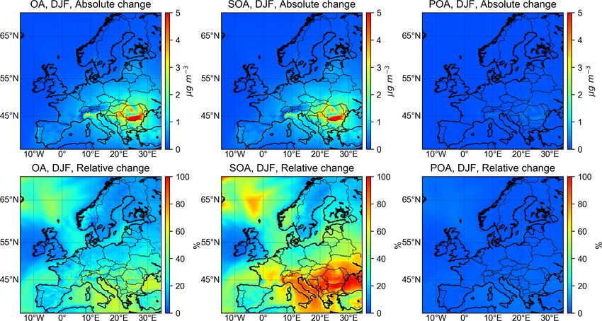
1682                 J. Jiang et al.: Influence of biomass burning vapor wall loss correction on modeling organic aerosols

among which residential biomass burning has been recog-            son et al., 2007). Nevertheless, recent studies have shown
nized as the dominant source for both primary (POA) and            that vapor wall losses lead to even larger variability in SOA
secondary (SOA) organic aerosols in Europe during winter-          yields according to different chamber conditions and pre-
time (Butt et al., 2016; Jiang et al., 2019b; Qi et al., 2019).    cursor species (Akherati et al., 2019; Cappa et al., 2016).
Despite its substantial contribution to OA, biomass burning        On the other hand, some studies took vapor wall loss cor-
OA is largely underestimated by chemical transport models          rections into account in CTMs using the SOA yields gener-
(CTMs) (Ciarelli et al., 2017a; Hallquist et al., 2009; Robin-     ated from the statistical oxidation model (SOM). Cappa et
son et al., 2007; Theodoritsi and Pandis, 2019; Woody et al.,      al. (2016) and Akherati et al. (2019) used the traditional two-
2016).                                                             product model to fit vapor-wall-loss-corrected SOA yields
   Many efforts have been devoted to understanding and di-         and applied the yields in the regional CTM UCD/CIT (Uni-
minishing the gap between modeled and observed OA from             versity of California at Davis/California Institute of Technol-
biomass burning. One of the major reasons for underesti-           ogy). They reported, however, that the two-product fits might
mated OA is the absence of semi-volatile organic compounds         not be sufficiently robust. Furthermore, Hodzic et al. (2016)
(SVOCs) from residential biomass burning in the current            used a vapor-wall-loss-corrected VBS parameterization in
emission inventories (Denier van der Gon et al., 2015). A          the global model GEOS-Chem based on chamber experi-
smog chamber study showed that the precursors tradition-           ments conducted on individual precursors, which are highly
ally included in CTMs account for only ∼ 3 %–27 % of the           dependent on the experimental conditions. Each of these
observed SOA from residential biomass burning (Bruns et            studies clearly called for a better assessment of the uncer-
al., 2016). In order to compensate for the effects from miss-      tainties across the entire range of precursor compounds as
ing precursors, various modeling studies have treated POA          well as under different chamber conditions.
as semi-volatile and adopted different scaling approaches to          Here, we (1) developed a VBS-based box model and fit
calculate SVOC and IVOC emissions. The most commonly               the vapor-wall-loss-corrected SOA yields of biomass burn-
used method is to increase the POA emissions by a factor           ing IVOCs based on 14 chamber experiments under different
of 3 (Ciarelli et al., 2017a; Fountoukis et al., 2014; Jiang et    temperature and emission loads, (2) implemented the vapor-
al., 2019b; Tsimpidi et al., 2010), while recent studies have      wall-loss-corrected VBS parameters in the regional chemical
also developed new profiles based on nonmethane organic            transport model Comprehensive Air Quality Model with ex-
compounds (NMOCs) (Cai et al., 2019; Lu et al., 2018).             tensions (CAMx), and (3) investigated the role of vapor wall
However, an increasing number of laboratory experimental           loss correction in model performance by comparing mod-
studies have found that SVOC and IVOC emissions have               eled organic aerosols from traditional and modified VBS
high variability depending on different burning conditions         OA schemes with ambient observations at multiple Euro-
and fuel types (Hatch et al., 2015, 2017; Jen et al., 2019;        pean sites. Biomass burning in this study refers to residential
Koss et al., 2018; Sekimoto et al., 2018), and the estima-         biomass burning, while wildfires and prescribed burning are
tion of SVOCs and IVOCs in modeling studies remains to             not included.
be improved. Meanwhile, increasing evidence from chamber
experiments has demonstrated that losses of semi-volatile va-
pors to chamber walls could lead to a substantial underesti-       2     Parameterization method
mation of OA (Akherati et al., 2020; Bertrand et al., 2018;
Bian et al., 2015; Krechmer et al., 2016; Loza et al., 2010;       2.1    Chamber experimental data
Matsunaga and Ziemann, 2010; Zhang et al., 2014). Unlike
particle wall losses – which are routinely corrected in cham-      The parameterization of the VBS scheme was based on ex-
ber studies – the effects of vapor wall losses are rarely inves-   perimental data from two smog chamber campaigns in 2014–
tigated and considered in modeling practices.                      2015. It includes 14 experiments conducted under various
   Zhang et al. (2014) reported that vapor wall losses may         temperature conditions (−10, 2, 15 ◦ C) and covered a wide
lead to an underestimation of SOA by a factor of 1.1–4.2, de-      range of emission loads (from 19 to 284 µg m−3 ). Emissions
pending on different NOx conditions. This factor has been          were generated by combustion of beechwood in three dif-
adopted by several CTM studies to scale up the yields of           ferent woodstoves, including conventional and modern burn-
SOA. For instance, Baker et al. (2015) tested the sensitiv-        ers, manufactured in 2002–2010. Beechwood is selected as
ity of CMAQ to vapor wall loss by increasing the yields            it is one of the major forest types in Europe, and beech-
of semi-volatile gases by a factor of 4, with the traditional      wood is widely used for residential heating and cooking in
two-product approach used for OA simulations. This factor          Europe. Although different biomass fuel types may largely
was also implemented in a box model with a volatility basis        affect the emitted organic gas species and affect SOA for-
set (VBS) scheme (Hayes et al., 2015), which distributed or-       mation, a recent study showed that the effect of biomass
ganic species into logarithmically spaced volatility bins, and     fuel type on SOA formation is much smaller than the ef-
was shown to improve the model performance for predicting          fects of initial organic mass (OM) load and hydroxyl (OH)
SOA (Donahue et al., 2011, 2006; Hodzic et al., 2010; Robin-       radical exposure (Lim et al., 2019). The organic gases cover-

Geosci. Model Dev., 14, 1681–1697, 2021                                            https://doi.org/10.5194/gmd-14-1681-2021
J. Jiang et al.: Influence of biomass burning vapor wall loss correction on modeling organic aerosols                         1683

ing 86 intermediate-volatility and semi-volatile organic com-       cles, kw is the rate constant of vapor lost to the wall, kdil is
pounds (IVOCs and SVOCs), which are SOA precursors,                 the dilution rate, and Ceqi,p and Ceqi,w represent the gas-phase
were measured by a proton-transfer-reaction time-of-flight          equilibrium concentrations to the aerosol particles and cham-
mass spectrometer (PTR-ToF-MS). The PTR-ToF-MS was                  ber wall surface, respectively:
operated under standard conditions in H3 O+ mode, as in-
troduced in Stefenelli et al. (2019). A common set of 263
ions was extracted from the measurements, and among these
                                                                    dCi
ions, 86 showed clear decay with time and were identified               = P · ζi − kcs Ci − Ceqi,p
as potential SOA precursors. These are listed in Table S1 of         dt

Stefenelli et al. (2019). The aerosol evolution was monitored           − kw Ci − Ceqi,w − kdil · Ci .                          (1)
by a high-resolution time-of-flight aerosol mass spectrometer
(HR-ToF-AMS). The particle wall loss has been corrected as
described in Stefenelli et al. (2019). The conditions of each
chamber experiment are shown in Table S1. A more detailed           The production rates of oxidized organic gases (P ) are used
description of the experiments can be found in Stefenelli et        as inputs of the box model. They are determined by the con-
al. (2019), Bertrand et al. (2017), and Bruns et al. (2016).        sumption rates of precursors measured by PTR taking into
                                                                    account their dilution. ζi represents the mass fraction of pri-
2.2   VBS box model                                                 mary and oxidation products in a volatility bin i. ζi of POA
                                                                    from biomass burning is obtained from May et al. (2013),
A VBS box model was developed to simulate the formation             with values of 0.2, 0.1, 0.1, 0.2, 0.1, and 0.3 for compounds in
and evolution of primary and secondary OA in the chamber.           each volatility bin. ζi of oxidation products is assumed to fol-
In the model, we assumed that the condensable gases gener-          low a kernel normal distribution as a function of log C ∗ , ζ ∼
ated from oxidation of the precursors could (1) partition to        N (µ, σ 2 ), where µ is the median value of log C ∗ and σ is
the particle phase, (2) be lost on the chamber wall, and/or         the standard deviation, which will be optimized as described
(3) be diluted by other gases injected into the smog chamber.       in Sect. 2.3. The assumption of a normal distribution could
CAMx includes four types of precursors from anthropogenic           ensure positive ζi values, allow constraining the total mass
sources, i.e., toluene, xylene, benzene, and IVOCs, which in-       fraction of the certain surrogate to equal 1, and reduce the
cludes all the other unspeciated organic gases. According to        model’s degree of freedom significantly, as reported in Ste-
our measurements, the traditional anthropogenic precursors          fenelli et al. (2019). The time series of kdil is obtained from
toluene, xylene, and benzene only account for ∼ 15 % of the         Stefenelli et al. (2019). The kcs of each experiment is ob-
total organic gases. To facilitate the implementation of the        tained from Bertrand et al. (2018). The kw varies significantly
optimized parameters in CAMx, all the measured SOA pre-             depending on the chamber conditions such as the chamber
cursors including the traditional ones were lumped into one         size and relative humidity. Zhang et al. (2014) reported kw
surrogate as IVOCs with the same reaction rate and volatility       values of 2.5 × 10⁻⁴ s−1 and 1 × 10⁻⁴ s−1 for toluene and
distribution. In comparison, Stefenelli et al. (2019) assigned      other VOCs, respectively, while it is much higher in recent
the same set of compounds to six different classes accord-          studies, such as 1.2 × 10⁻³ to 2.4 × 10⁻³ s−1 in Krechmer
ing to their properties (reaction rates, expected SOA yields,       et al. (2016), 1.28 × 10⁻³ s−1 in Akherati et al. (2020), and
etc.) as well as their origins and occurrence in the emissions.     ∼ 1 × 10⁻³ to 3.3 × 10⁻³ s−1 in Bertrand et al. (2018). To
These included furans and methoxy-phenols from the pyroly-          cover the wide range of vapor wall loss, we tested three kw
sis of cellulose and lignin, respectively, single-ring and poly-    values of 0.0020, 0.0033, and 0.0040 s−1 based on the con-
aromatic hydrocarbons from flaming combustion, and oxy-             ditions of our chamber. A base case was also developed by
genated non-aromatic compounds with fewer and more than             assuming there is no vapor wall loss in the chamber (kw = 0).
six carbon atoms. The current lumping approach of all these         The condensation of a species in the particle phase (Cp ) can
species into one surrogate, despite variations in their prop-       then be described by Eq. (2).
erties, is more adapted for implementation into CAMx and
for assessing vapor wall losses with additional parameters
included in the box model. The organic compounds were dis-
                                                                    dCi,p
tributed into six logarithmically spaced volatility bins corre-           = kcs Ci − Ceqi,p − kdil · Ci,p                       (2)
sponding to saturation concentrations of 10−1 , 100 , 101 , 102 ,    dt
103 , and 104 µg m−3 . The change in the organic gas concen-
tration (C) for a constituent within the volatility bin i (Ci )
can be described by Eq. (1), where P is the production of or-       Following the partitioning model of Pankow (1994), the gas-
ganic gas (OG) in the chamber due to oxidization of precur-         phase concentrations at equilibrium with respect to the parti-
sors, kcs is the condensation sink (s−1 ) describing the speed      cle phase (Ceqi,p ) and to the chamber wall (Ceqi,w ) are deter-
of condensable gases condensing on existing aerosol parti-          mined by their partitioning coefficients ξi and ξi,w (Donahue

https://doi.org/10.5194/gmd-14-1681-2021                                              Geosci. Model Dev., 14, 1681–1697, 2021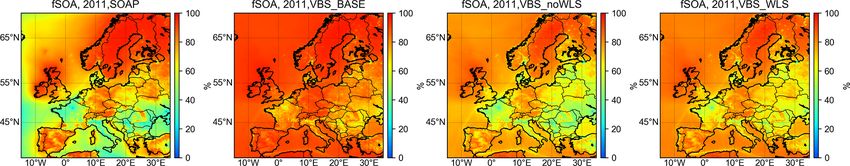
1684                 J. Jiang et al.: Influence of biomass burning vapor wall loss correction on modeling organic aerosols

et al., 2009), as shown in Eqs. (3) and (4).                        reaching 20. The GA is conducted using the genetic algo-
                                                                    rithm solver in the MATLAB R2019a Global Optimization
                                             C ∗ −1

                                                                    Toolbox (The MathWorks, Inc).
Ceqi,p = (Ci,g + Ci,p ) · [1 − ξi ], ξi = 1 + i              (3)
                                             COA
Ceqi,w = (Ci,g + Ci,w ) · [1 − ξi,w ],                              3     Modeling approach
                 C ∗ −1

 ξi,w = 1 + i                                                (4)    3.1    Regional chemical transport model CAMx
                Cwall
                                                                    The regional model CAMx version 6.50 (Ramboll, 2018)
Here, C ∗ represents the saturation concentration, COA is the
                                                                    was used to model organic aerosol in Europe (15◦ W–35◦ E,
wall-loss-corrected OA concentration measured by the AMS,
                                                                    35–70◦ N) for the whole year of 2011, with a horizontal
and Cwall is the equivalent organic mass concentration at
                                                                    resolution of 0.25◦ × 0.125◦ and 14 terrain-following ver-
the wall determined in Bertrand et al. (2018). The Clausius–
                                                                    tical layers from ∼ 20 m above the ground up to 460 hPa.
Clapeyron equation (Eq. 5) was applied to take into account
                                                                    The Carbon Bond 6 Revision 2 (CB6r2) gas-phase mecha-
the effects of temperature on C ∗ :
                                                                    nism (Hildebrandt Ruiz and Yarwood, 2013) was selected.
                                                                    The gas–aerosol partitioning of inorganic aerosols was sim-

  ∗     ∗    T0          1Hvap /8.314
C = CT 0 ·       · exp                  ,                 (5)       ulated by the ISORROPIA thermodynamic model (Nenes et
             T           1/T0 − 1/T
                                                                    al., 1998). For organic aerosols, several OA schemes, includ-
where CT∗ 0 is the mass saturation concentration under the          ing both the traditional two-product approach (SOA chem-
reference temperature (T0 ). T is the temperature of each           istry partitioning scheme, SOAP) and the VBS scheme with
experiment, while T0 equals 298 K. 1Hvap (J) is the en-             different parameterizations, were applied (see Sect. 3.2).
thalpy of vaporization at the reference temperature, and               The meteorological parameters were prepared with the
8.314 is the universal gas constant (J mol−1 K−1 ). 1Hvap =         Weather Research and Forecasting model (WRF ver-
{70 000 − 11 000 × log C ∗ } is adopted for the primary set         sion 3.7.1; Skamarock et al., 2008) based on the 6 h European
(May et al., 2013), while 1Hvap of the oxidized products is         Centre for Medium-Range Weather Forecasts (ECMWF) re-
determined during model optimization. The Cwall was deter-          analysis global data (Dee et al., 2011). The meteorological
mined in previous studies to be of the order of a few mil-          parameters were evaluated and reported in a previous study
ligrams per cubic meter (mg m−3 ; Bertrand et al., 2018). In        (Jiang et al., 2019a), which showed that most of the meteoro-
this study, we run the box model for three different Cwall val-     logical parameters met the criteria for meteorological model
ues (1, 5, 25 mg m−3 ) with a reference temperature of 2 ◦ C        performance by Emery (2001). The initial and boundary
(275.15 K) according to Bertrand et al. (2018).                     conditions were obtained from the global model MOZART-
                                                                    4/GEOS-5 (Horowitz et al., 2003). Inputs of ozone column
2.3    Model optimization                                           densities were produced based on the Total Ozone Map-
                                                                    ping Spectrometer (TOMS) data by the National Aeronau-
The model is optimized to constrain the volatility distribution     tics and Space Administration (NASA, https://acd-ext.gsfc.
(as a function of log C ∗ , ζ ∼ N (µ, σ 2 )) and 1Hvap of the ox-   nasa.gov/anonftp/toms/omi/data/Level3e/ozone/, last access:
idized products. A genetic algorithm (GA) is used to find the       17 March 2021), and the photolysis rates were then cal-
best-fit parameters leading to the lowest average root mean         culated by the Tropospheric Ultraviolet and Visible (TUV)
square error (RMSE) and mean bias (MB) between modeled              Radiation Model version 4.8 (NCAR, 2011). The source-
and measured OA concentrations for all 14 experiments. The          specific anthropogenic emissions were based on the Euro-
genetic algorithm is a metaheuristic algorithm inspired by          pean emission inventory TNO-MACC-III (Monitoring At-
the natural selection process to generate optimized solutions       mospheric Composition and Climate) (Kuenen et al., 2014).
(Mitchell, 1996). It begins by creating an initial population of    The biogenic emissions (isoprene, monoterpenes, sesquiter-
individual solutions (20 different combinations of µ, σ , and       penes, soil NO) were simulated by the PSI model devel-
1Hvap here) within certain upper and lower bounds, called           oped at the Laboratory of Atmospheric Chemistry at the Paul
parents. The performance of each solution is evaluated by a         Scherrer Institute (Andreani-Aksoyoglu and Keller, 1995;
fitness function, which is the sum of RMSE and MB between           Jiang et al., 2019a; Oderbolz et al., 2013). More details about
the modeled and measured OA concentrations of 14 experi-            the model inputs can be found in our previous studies per-
ments in this study. A new generation of solutions is then          formed using the same input data (Jiang et al., 2019a, b).
formed either by making random changes to a single parent
(called mutation) or by combining the vector entries of a pair      3.2    Parameterization of OA schemes
of parents (called crossover). The process will be repeated
until reaching the stopping conditions, which involves either       To investigate the effects of vapor-wall-loss-corrected yields
the number of iterations reaching 50 or the stall generations       and to compare to other modifications and/or parameteriza-
(generation with no significant change in the fitness function)     tions that are currently strongly debated in the community,

Geosci. Model Dev., 14, 1681–1697, 2021                                             https://doi.org/10.5194/gmd-14-1681-2021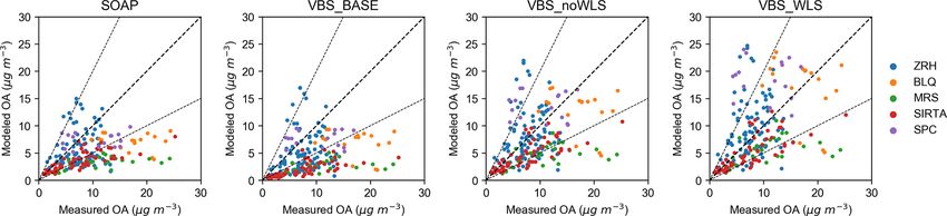
J. Jiang et al.: Influence of biomass burning vapor wall loss correction on modeling organic aerosols                                             1685

Table 1. Description of the different OA schemes.

                     OA scheme             IVOBa emissions            kOH for IVOB                 SOA yields for IVOB
                                                                      (cm3 molec−1 s−1 )           (ppm / ppm)b
                     SOAP                  4.5· POA_BB                1.34                         /c
                     VBS_BASE                                         4.0                          [0.081, 0.135, 0.800, 0.604, 0.0]
                     VBS_3POA                                         4.0                          [0.081, 0.135, 0.800, 0.604, 0.0]
                     VBS_noWLS             12· POA_BB                 1.5                          [0.014, 0.036, 0.076, 0.136, 0.44]
                     VBS_WLS                                          1.5                          [0.078, 0.118, 0.157, 0.177, 0.312]
                   a IVOB is the abbreviation for “IVOCs from biomass burning” in CAMx.
                   b The yield values correspond to volatility bins with saturation concentrations of 10−1 , 100 , 101 , 102 , and 103 µg m−3 .
                   c SOAP does not separate IVOCs from biomass burning and other anthropogenic sectors, and therefore it is not comparable
                   with the SOA yields for IVOBs.

five simulations with different OA schemes were conducted                                    posed to be a reference case representing the commonly
in this study (Table 1). Besides VBS_WLS, which uses                                         used approach without vapor wall loss, and therefore
the optimized parameterization with vapor wall loss correc-                                  we adopted the routine approach of multiplying the
tion for the biomass burning sector, SOAP and VBS_BASE                                       POA emissions by a factor of 3 to offset the influence
represent the two standard parameterizations in CAMx;                                        of missing SVOC emissions. This approach has been
VBS_3POA represents a common approach to offset the                                          widely used in modeling studies (Ciarelli et al., 2016,
missing SVOC emissions in recent modeling studies without                                    2017a; Shrivastava et al., 2011; Tsimpidi et al., 2010).
vapor wall loss, and VBS_noWLS is another reference case                                     All the other parameters were kept the same as the
without vapor wall loss, which uses exactly the same param-                                  standard VBS parameterization in CAMx v6.50. The
eters as VBS_WLS except for the SOA yields from IVOCs.                                       VBS_BASE IVOC emissions were adopted here.
Details about each OA scheme are introduced below.
                                                                                          – VBS_WLS. The VBS_WLS used the optimized pa-
  – SOAP. The SOAP (SOA chemistry partitioning) module                                      rameters by the VBS box model, including the emis-
    is a semi-volatile equilibrium scheme based on the tra-                                 sions and vapor-wall-loss-corrected yields for IVOCs
    ditional two-product approach. POA emissions are as-                                    from residential biomass burning, and the 1Hvap
    sumed to be inert in SOAP. The updated parameteriza-                                    of the oxidized products. The modified parameters
    tion of SOAP2.1 in CAMx v6.50 used the aerosol yield                                    for volatility-bin-specific yields and 1Hvap of the
    data that correct for vapor wall losses in smog chamber                                 oxidized products from IVOCs can be found at
    experiments based on Zhang et al. (2014).                                               https://doi.org/10.5281/zenodo.3998342 (Jiang, 2020).
                                                                                            The optimized mass yields in the box model were
  – VBS_BASE. The VBS_BASE used the standard VBS                                            converted to molar yields using the default molecular
    parameterization in CAMx v6.50. The IVOC emissions                                      weights in CAMx (Table 1). Both the optimized and
    from different sources were calculated based on the lit-                                default molar yields have a sum larger than 1 as the
    erature. IVOCs from gasoline and diesel vehicles were                                   VBS scheme accounts for both oxygenation and frag-
    calculated as 25 % and 20 % of NMVOC emissions                                          mentation (Koo et al., 2014). The reaction rate with
    from gasoline and diesel vehicles, respectively (Jathar                                 OH (kOH ) was calculated based on the measurements
    et al., 2014). IVOC emissions from residential biomass                                  following Stefenelli et al. (2019). Based on the cham-
    burning were estimated as 4.5 times POA emissions                                       ber measurements, the IVOC emissions from residen-
    based on Ciarelli et al. (2017a). The IVOC emissions                                    tial biomass burning are ∼ 13.7 times the primary OM
    from other anthropogenic sources were calculated as 1.5                                 load (Fig. S1), among which the traditional precursors
    times POA as proposed by Robinson et al. (2007).                                        in CAMx from biomass burning (toluene, xylene, and
                                                                                            benzene) account for ∼ 15 % of the total emissions. To
  – VBS_3POA. An increasing number of experimental and
                                                                                            avoid double counting of these traditional precursors,
    modeling studies have reported a considerable contri-
                                                                                            which are already included in the emission inventory,
    bution of semi-volatile organic compounds (SVOCs)
                                                                                            we applied a factor of 12 to calculate the IVOC emis-
    to SOA formation (Bruns et al., 2016; Ciarelli et al.,
                                                                                            sions from biomass burning. The IVOC emissions from
    2017b; Denier van der Gon et al., 2015; Hatch et al.,
                                                                                            other sources were estimated by using the same ap-
    2017; Woody et al., 2015), while SVOCs are absent
                                                                                            proach as in VBS_3POA.
    in the current emission inventories. Despite consider-
    able variability of SVOC emissions from biomass burn-                                 – VBS_noWLS. The VBS_noWLS was designed as a ref-
    ing according to recent studies, the VBS_3POA is sup-                                   erence for VBS_WLS, which adopted the same pa-

https://doi.org/10.5194/gmd-14-1681-2021                                                                       Geosci. Model Dev., 14, 1681–1697, 2021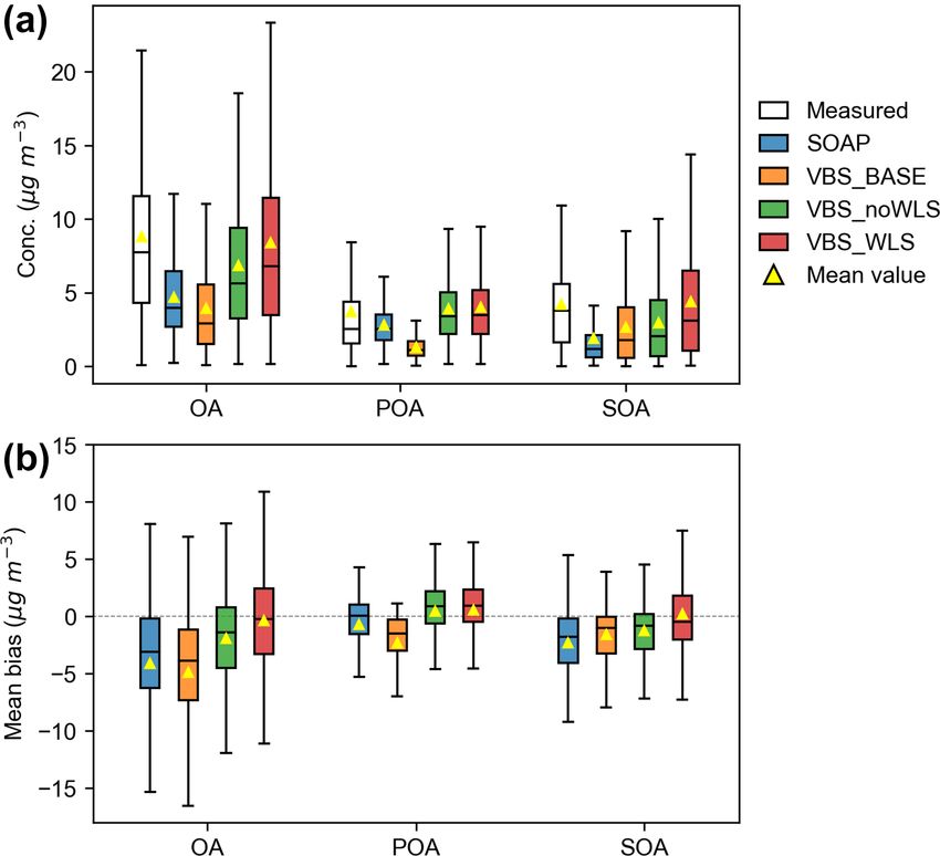
1686 J. Jiang et al.: Influence of biomass burning vapor wall loss correction on modeling organic aerosols
rameters as VBS_WLS except for the yields. The as temperature and chamber conditions. While the model
VBS_noWLS used the fitted yields from the box model simulation without vapor wall loss correction largely over-
assuming that there is no vapor wall loss (kw = 0). estimates OA at the initial time point and underestimates
the final OA (Fig. S3), the agreement between the mod-
3.3 Model evaluation eled and measured trends improved when the vapor wall loss
was taken into account. The mean bias (MB) and root mean
The general model performance for the major air pollu- square error (RMSE) between the modeled and observed OA
tants (SO2 , NO2 , O3 , PM2.5 ) was reported in our previ- in 14 experiments are 6.7 and 42.2 µg m−3 for the case under
ous study (Jiang et al., 2019b), which was comparable to median chamber conditions, which are 48 % and 12 % lower
other modeling studies in Europe. OA measurements and than in the case without vapor loss correction (MB = −12.8,
source apportionment studies using positive matrix factor- 47.8 µg m−3 ). To investigate the role of vapor wall loss in
ization (PMF) analysis from five Aerodyne aerosol chemi- modeled OA, another set of simulations was performed in
cal speciation monitor (ACSM) or aerosol mass spectrome- which we used the same optimized parameterization under
ter (AMS) stations in the winter of 2011 were used to evalu- the median chamber conditions but set kw = 0. In these cases,
ate modeled primary and secondary organic aerosol by dif- the modeled OA concentrations (dashed line in Fig. 1) were
ferent OA schemes: Zurich (Canonaco et al., 2013), Mar- based on the assumption that there is no vapor wall loss. The
seille (Bozzetti et al., 2017), the SIRTA (Site Instrumental wall loss ratio Rwall , which is defined as the ratio between
de Recherche par Télédétection Atmosphérique) facility lo- the modeled OA concentration without (kw = 0) and with
cated in the Paris region (Zhang et al., 2019), and Bologna (kw = 0.0033 s−1 , Cwall = 5 mg m−3 ) vapor wall loss, was
and San Pietro Capofiume (SPC) (Paglione et al., 2020). For calculated for the end point of each experiment (Fig. 1c). The
Zurich and SIRTA, only data collected from late autumn to Rwall values varied from 1.5 (Exp2) to 3.2 (Exp11) among the
early spring (January, February, March, November, and De- 14 experiments and showed a clear dependence on the initial
cember) – when emissions from biomass burning are rela- OA loads.
tively high – were used for the statistical analysis, although To further understand the factors influencing Rwall , we
the observations covered longer time periods. The spatial dis- conducted a series of model simulations with and without va-
tribution and observation periods of each station are shown in por wall loss under different initial organic mass loads, tem-
Fig. S2. Statistical metrics, including mean bias (MB), mean perature, and condensation sink inputs (Fig. 2). Higher kw
error (ME), root mean square error (RMSE), mean fractional and Cwall lead to higher Rwall values for all the cases, and dif-
bias (MFB), and mean fractional error (MFE), between mod- ferent chamber conditions (kw , Cw ) could result in a different
eled and observed primary and secondary OA were calcu- Rwall by a factor of 1.2–1.6, depending on different temper-
lated. ature, OM loads, and condensation sinks. The Rwall values
generally decrease with increasing initial OM loads, which
4 Results and discussion is consistent with the fact that Rwall values for Exp8–14 are
higher than Exp1–7. The increased Rwall with the increasing
4.1 Modeled and measured OA from chamber temperature explains why Exp10 through Exp14 (T = 15 ◦ C)
experiments have higher Rwall than Exp8 and Exp9 (T = −10 ◦ C), while
they have similar OM load levels. The condensation sink is
The optimized parameters were then applied to the box inversely correlated with Rwall , indicating that the higher the
model to simulate OA production for 14 chamber ex- rate of condensable gases condensing on the existing parti-
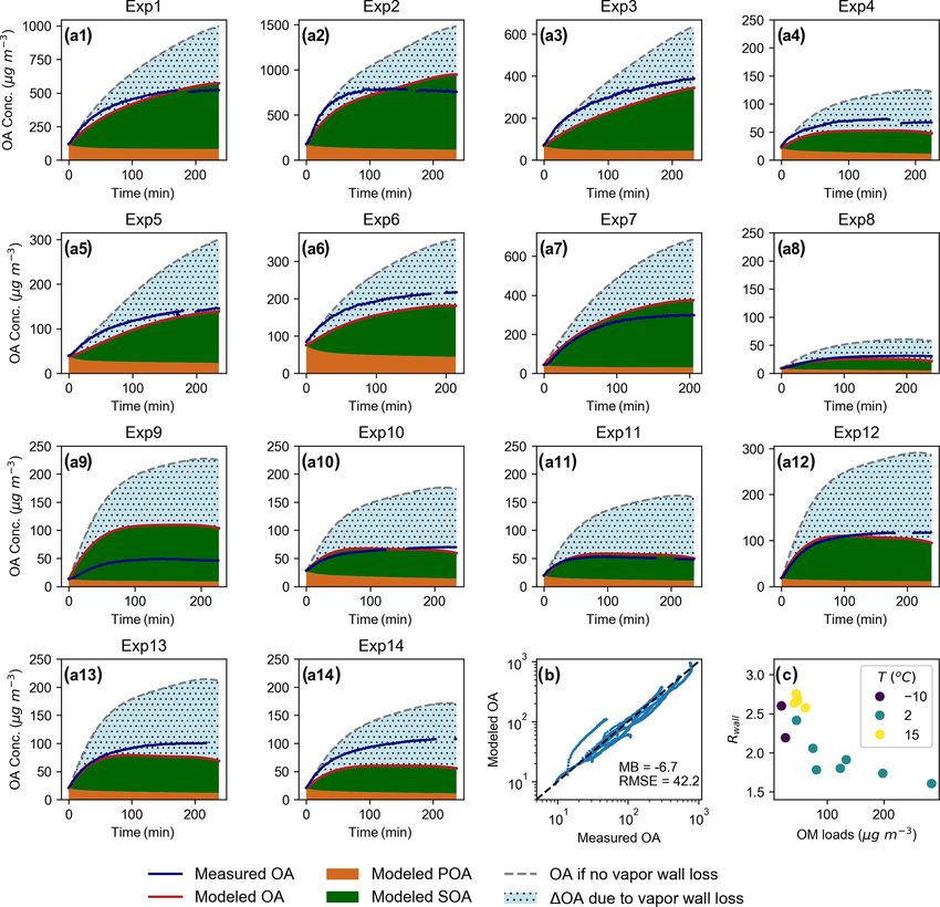
periments. Figure 1 shows the comparison between mea- cles, the lower the vapor loss to the chamber wall, and there-
sured OA and modeled primary and secondary OA under fore the lower the effect of vapor wall loss on modeled OA.
the median chamber conditions (kw = 0.0033 s−1 , Cwall = The optimized volatility distribution for the secondary
5 mg m−3 ) for each experiment. The model reproduces the condensable gases from biomass burning (ppm per ppm
process of OA formation for most of the experiments well, IVOC) based on different wall loss assumptions (kw > 0 or
except for experiments no. 9 and no. 14, which have rel- kw = 0) is displayed in Fig. 3a. The optimized yields con-
atively lower OM loads (26 and 48 µg m−3 for Exp9 and sidering vapor wall loss lead to a 3.3 times higher mass in
Exp14, respectively). This can be partially explained by the the low-volatility bins (log C ∗ ≤ 0) compared to that assum-
different weighting impact for experiments with high or low ing kw = 0, indicating significant effects of vapor wall loss
OM loads. The experiments with higher OM loads normally correction on predicting SOA production. To give a more di-
have larger MB and RMSE at the beginning of optimiza- rect view of the effects of vapor wall loss on the SOA yield,
tion and therefore have a higher impact during the model we integrated the mass of SOA for all the volatility bins at
optimization. A direct consequence is that the optimized pa- 298 K (Fig. 3b). The mass yield under the median cham-
rameters would work better for experiments with higher OM ber conditions for vapor wall loss (kw = 0.0033 s−1 , Cwall =
loads. However, the model performance in each experiment 5 mg m−3 ) is higher than the base case without considering
could also be influenced by a series of other factors such the vapor wall loss about by factors of 4.9 (when COA =
Geosci. Model Dev., 14, 1681–1697, 2021 https://doi.org/10.5194/gmd-14-1681-2021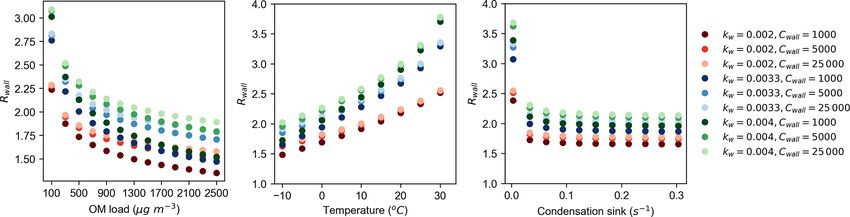
J. Jiang et al.: Influence of biomass burning vapor wall loss correction on modeling organic aerosols                           1687

Figure 1. Comparison between measured and modeled OA with an optimized parameterization under kw = 0.0033 s−1 and Cwall =
5 mg m−3 (a, b). Relation between the end-point wall loss factor Rwall of each experiment and initial OM loads under different temper-
ature (c). The gray dashed lines in (a) represent modeled OA with the same parameterization but kw = 0.

0.1 µg m−3 ) to 1.9 (when COA = 1000 µg m−3 ). The influ-            stations in winter. The statistical results are shown in Table 2,
ence of vapor wall loss on mass yield decreases with decreas-        and the distributions of OA concentrations and the mean bias
ing temperature. At 0 ◦ C, the mass yield with vapor wall loss       between modeled and measured primary and secondary OA
correction is higher than the base case by factors of 4.3 (when      are displayed in Fig. 4. OA is underestimated overall with all
COA = 0.1 µg m−3 ) to 1.7 (when COA = 1000 µg m−3 ).                 OA schemes. The VBS schemes lead to a better model per-
                                                                     formance than the two-product approach SOAP, except for
4.2   Performance of CAMx with different OA schemes                  VBS_BASE with the default VBS parameterization. These
                                                                     results are consistent with a previous study using CAMx
                                                                     (Meroni et al., 2017), in which the better performance of
The modeled OA concentrations with different OA schemes
                                                                     SOAP compared to the default VBS was reported as a result
were compared with measurements from five ACSM/AMS

https://doi.org/10.5194/gmd-14-1681-2021                                                Geosci. Model Dev., 14, 1681–1697, 2021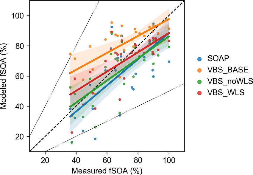
1688                  J. Jiang et al.: Influence of biomass burning vapor wall loss correction on modeling organic aerosols

Figure 2. Dependence of the wall loss factor Rwall (COA, kw =0 /COA, optimalkw ) on initial organic mass load, temperature, and condensation
sink.

Figure 3. Optimized yield factors (a) and the mass yield of SOA from biomass burning at 298 K (b) with and without vapor wall loss
correction. The blue bars (a) and line (b) with vapor wall loss refer to median chamber conditions with kw = 0.0033 s−1 and Cwall =
5 mg m−3 .

of error compensation. The improved performance of modi-                corrected yields for biomass burning improve the model per-
fied VBS (3POA, noWLS, WLS) for OA mainly comes from                    formance in February and March, while there is an overesti-
the contribution of SOA (Table 2). The modeled SOA by                   mation of OA and SOA for all the OA schemes in November
3POA and noWLS is very similar, and therefore the analy-                (Fig. S4a). The largest contribution to OA during this pe-
sis below will focus on the comparison between noWLS and                riod was found to be from biogenic SOA, which was poten-
WLS, for which the only difference is that WLS uses vapor-              tially overestimated due to overestimated temperatures dur-
wall-loss-corrected yields for IVOCs from biomass burning,              ing the same time period (Jiang et al., 2019b). Bologna and
while noWLS uses the fitted yields assuming no vapor wall               SPC are located in the Po Valley where biomass burning con-
loss (kw = 0). WLS reduces the MFB between the modeled                  tributes most to winter OA (Jiang et al., 2019b), and therefore
and measured SOA from 52.5 % in noWLS to 20.0 %. WLS                    higher effects from vapor wall loss correction on SOA are
shows a better average MB than noWLS; however, it also                  observed compared to other sites. At SPC, fog scavenging
increases the upper whisker of the MB (Fig. 4b), largely af-            processes played an important role in OA during the mea-
fected by overestimated SOA in Bologna and SPC.                         surements (Gilardoni et al., 2014); however, the meteoro-
   Limited by the availability of OA measurements, the ef-              logical model failed to reproduce the fog events due to the
fects of vapor wall loss correction on model performance                coarse resolution in this study (Jiang et al., 2019b). Conse-
present a clear site dependence in this study. The modeled              quently, both VBS_WLS and noWLS lead to an overestima-
and measured daily average OA concentrations at each site               tion of OA and SOA, while SOAP and VBS_BASE show
are shown in Fig. 5. The temporal variations of primary                 better performance, probably due to compensation for errors
and secondary OA at these sites can be found in Fig. S4.                (Fig. S4e). In Bologna, a significant overestimation of tem-
VBS_WLS leads to the best performance for both OA and                   perature was found on 2 to 6 December (Jiang et al., 2019b),
SOA in Marseille and SIRTA, in spite of an overall un-                  leading to a significant underestimation of SOA for all the
derestimation (Fig. S4b, c). In Zurich, the vapor-wall-loss-            OA schemes (Fig. S4d). Excluding this period, the mod-

Geosci. Model Dev., 14, 1681–1697, 2021                                                   https://doi.org/10.5194/gmd-14-1681-2021
J. Jiang et al.: Influence of biomass burning vapor wall loss correction on modeling organic aerosols 1689
Table 2. Statistical results for model performance in simulating OA, SOA, and POA. The number of daily average observations from five
ACSM/AMS stations is 216.
Species OA scheme MB ME RMSE MFB MFE r
(µg m−3 ) (µg m−3 ) (µg m−3 ) (%) (%)
OA SOAP −4.1 4.9 7.2 −44.3 65.3 0.38
VBS_BASE −4.9 5.6 7.9 −72.9 83.3 0.29
VBS_3POA −1.6 4.3 6.5 −12.4 51.7 0.42
VBS_noWLS −1.9 4.3 6.5 −17.4 52.7 0.41
VBS_WLS −0.4 4.6 6.9 −1.6 52.2 0.41
SOA SOAP −2.3 3.1 4.3 −77.8 98.3 0.12
VBS_BASE −1.6 2.8 4.1 −63.0 90.6 0.22
VBS_3POA −1.2 2.8 4.1 −51.1 84.3 0.23
VBS_noWLS −1.3 2.8 4.0 −52.5 84.9 0.24
VBS_WLS 0.2 3.2 4.6 −20.0 76.4 0.26
POA SOAP −0.7 1.9 3.1 4.4 56.7 0.49
VBS_BASE −2.3 2.5 4.0 −64.1 81.5 0.44
VBS_3POA 0.8 2.4 3.4 36.3 64.2 0.45
VBS_noWLS 0.4 2.2 3.2 30.1 61.9 0.45
VBS_WLS 0.6 2.3 3.3 32.4 62.5 0.45
emissions from biomass burning, which were estimated by
the same factor for the whole domain but were reported
to have substantial inter-country variations (Denier van der
Gon et al., 2015). Missing formation and removal processes
such as photolytic and heterogeneous oxidation in the model
could also result in different model performance for specific
sites. In addition, in spite of the advanced chamber measure-
ments we used to optimize the yield parameters covering a
wide range of precursor species and multiple temperature and
chamber conditions, the fitted vapor-wall-loss-corrected pa-
rameterization is still highly uncertain. To achieve a more ro-
bust parameterization and to further improve the model per-
formance for OA, more studies on SVOC and IVOC emis-
sions, as well as the formation and removal mechanisms of
SOA based on extensive laboratory studies and field observa-
tions with higher spatial and temporal coverage, are needed.
4.3 Effects of vapor wall loss correction on modeled
OA in Europe
Figure 4. Concentrations of measured and modeled OA, POA, and
SOA at five ACSM or AMS stations in winter (a) and mean bias for 4.3.1 OA
different OA schemes (b). The lines inside boxes represent median
values, and the yellow triangles represent mean values. The modeled OA results in Europe for the whole year of 2011
with different OA schemes were compared to investigate
the effects of OA schemes and the vapor wall loss correc-
eled SOA by VBS_WLS is 89 % higher than the measure- tion. Among all the sources, residential biomass burning con-
ments, while the modeled SOA concentrations by the other tributed 16.3 %–52.6 % POA and 5.9 %–28.9 % SOA in win-
schemes are closer to the measurements, with relative differ- ter (Jiang et al., 2019b), indicating the potential roles of va-
ences of −64 % for SOAP, −10 % for VBS_BASE, and 4 % por wall loss for the biomass burning sector. Figure 6 shows
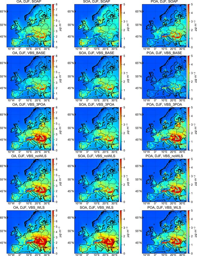
for VBS_noWLS. the modeled OA, SOA, and POA in winter (December–
The distinct performance of vapor-wall-loss-corrected January–February). VBS_WLS leads to the highest domain
VBS at different sites could arise from various factors. It average OA (2.3 µg m−3 ), which is 16.4 %, 26.2 %, 38.7 %,
might come from the high uncertainties of SVOC and IVOC and 106.6 % higher than VBS_3POA, VBS_noWLS, SOAP,
https://doi.org/10.5194/gmd-14-1681-2021 Geosci. Model Dev., 14, 1681–1697, 20211690 J. Jiang et al.: Influence of biomass burning vapor wall loss correction on modeling organic aerosols
Figure 5. Measured and modeled daily average OA using different OA schemes in winter. ZRH: Zurich, BLQ: Bologna, MRS: Marseille,
SIRTA: Paris SIRTA, SPC: San Pietro Capofiume.
and VBS_BASE, respectively. The VBS schemes generally (domain average 71.4 %–87.3 %) compared to SOAP (do-
produce higher OA than SOAP, except for the default param- main average 69.9 %) in most of the domain except for north-
eterization (VBS_BASE) in which the lack of SVOC emis- ern Europe, where SOAP produces high biogenic SOA. The
sions is not considered. However, SOAP leads to the second increased POA emissions to offset the missing SVOC emis-
highest SOA after VBS_WLS, especially in northern Eu- sions (3POA, noWLS, WLS) decrease the fSOA compared to
rope where monoterpene emissions from coniferous forests the default VBS parameterization (BASE), while the vapor
are relatively high. This is mostly because of the high ter- wall loss correction yields (WLS) result in ∼ 5.8 % higher
pene SOA yields in SOAP2.1, which were reduced in the fSOA than noWLS for the domain average, and the largest
later version of the CAMx model (CAMx v7.0, http://www. grid-scale increase reaches 43.4 % in the Balkans. The ab-
camx.com, last access: 17 March 2021). The vapor-wall- solute differences between fSOA for WLS and noWLS are
loss-corrected yields lead to increased SOA in large areas of relatively higher in rural areas than urban areas, where fSOA
central and southern Europe (Fig. 7). The largest difference is is lower due to high primary emissions.
predicted for the Po Valley and Romania regions with a high The modeled fSOA values were compared with mea-
residential biomass burning impact (Fig. S5). The overall surements from previous studies in Europe (Crippa et al.,
relative differences between VBS_WLS and VBS_noWLS 2014; Jiang et al., 2019b). The measured fSOA from the
are more than 80 %, and the highest grid-scale increment literature covered 18 sites and different seasons between
reaches 5.6 µg m−3 in the region of the Balkans. The mod- 2008 and 2011 (Table S2). SOAP tends to underestimate
eled POA concentrations are similar to those in the VBS case the fSOA, while VBS_BASE significantly overpredicts the
with correction for SVOC (3POA, noWLS, WLS), with do- fSOA (Fig. 9). Both WLS and noWLS tend to underestimate
main average concentrations ranging from 0.9 (noWLS) to the high fSOA and overestimate the low fSOA. VBS_WLS
1.1 (3POA) µg m−3 , and therefore no significant effects were has 5 % higher fSOA than VBS_noWLS and shows the
observed from vapor wall loss correction (Fig. 6). The POA highest agreement on the range of fSOA with the mea-
simulated by VBS_BASE (0.3 µg m−3 ) is even lower than surements and the average fSOA values (measured: 69.6 %;
SOAP (0.7 µg m−3 ), as POA is semi-volatile and could evap- VBS_WLS: 69.1 %). The largest improvements occur in
orate and react with oxidants to form secondary products in winter when the vapor-wall-loss-corrected yields of biomass
VBS, while SOAP assumes POA to be inert. burning emissions largely increase the SOA production.
The effects of different VBS schemes on OA are much
smaller in summer (Fig. S6). Despite a slight increase
from the VBS_BASE (1.2 µg m−3 ), the modeled OA by 5 Conclusions
the three modified VBS schemes is quite similar (1.4–
1.5 µg m−3 ). The effects of vapor-wall-loss-corrected yields In this study, we optimized the SOA yields for a VBS-based
for biomass burning emissions are negligible due to low box model using 14 chamber experiments with biomass
emissions in summer (Fig. S7). SOAP produced the highest burning and implemented the fitted VBS parameters (SOA
OA (2.1 µg m−3 ) in summer due to the high SOA yields from yields, IVOC emissions from biomass burning, and enthalpy
monoterpenes as explained before. of vaporization) in the regional air quality model CAMx
v6.5. The influence of the vapor wall loss correction on the
4.3.2 Fraction of SOA in OA model performance was investigated by comparing modeled
primary and secondary OA with traditional and modified OA
The effects of the updated VBS schemes on the fraction of schemes, including the two-product approach (SOAP), the
annual average SOA in total OA (fSOA = SOA / OA) are standard VBS (VBS_BASE), VBS with 3 times the POA
shown in Fig. 8. The VBS schemes lead to a higher fSOA to compensate for the missing SVOCs (VBS_3POA), VBS
Geosci. Model Dev., 14, 1681–1697, 2021 https://doi.org/10.5194/gmd-14-1681-2021J. Jiang et al.: Influence of biomass burning vapor wall loss correction on modeling organic aerosols 1691 Figure 6. Modeled OA, SOA, and POA in winter (DJF, December–January–February) by different OA schemes. https://doi.org/10.5194/gmd-14-1681-2021 Geosci. Model Dev., 14, 1681–1697, 2021
1692                J. Jiang et al.: Influence of biomass burning vapor wall loss correction on modeling organic aerosols

Figure 7. Differences in modeled OA, SOA, and POA in winter (DJF, December–January–February) by VBS schemes with (VBS_WLS)
and without (VBS_noWLS) vapor wall corrections.

Figure 8. Modeled fractions of annual mean SOA to total OA (fSOA) using different OA schemes. Modeled results for VBS_3POA are very
similar to VBS_noWLS and are therefore not shown here.

with vapor wall loss correction (VBS_WLS), and an addi-             spectively. The largest influence of vapor wall loss correc-
tional reference scenario with the same parameterizations as        tion was predicted in Romania where the VBS_WLS in-
in VBS_WLS except for using the default SOA yields from             creases SOA by ∼ 80 % compared to VBS_noWLS due to
biomass burning IVOCs (VBS_noWLS).                                  high emissions from residential biomass burning. VBS_WLS
   The vapor wall loss correction increases the mass dis-           also leads to the highest agreement with measurements for
tributed in the low-volatility bins (log C ∗ ≤ 0) by a factor       the SOA fraction in OA (fSOA) from the literature.
of 4.3 and increases the SOA yields by a factor of 1.9–4.9             The optimized parameterization with vapor wall loss cor-
(at 298 K). Comparison of the modeled results with different        rection in this study is expected to provide some insight to
OA schemes to field measurements from five ACSM/AMS                 improve SOA underestimation in CTMs. Despite the overall
stations in Europe in winter suggests that VBS_WLS gen-             improvement of model performance for predicting SOA, the
erally has the best performance to predict OA, which lowers         VBS_WLS was found to increase the mean bias at specific
the highest mean fractional bias from −72.9 % (VBS_BASE)            sites compared to noWLS. To achieve a more robust param-
to −1.6 % for OA and from −77.8 % (SOAP) to 20.0 % for              eterization and to further improve the model performance,
SOA. In Europe, the VBS_WLS produces the highest do-                complementary studies on SVOC and IVOC emissions, as
main average OA in winter (2.3 µg m−3 ), which is 106.6 %           well as on the formation and removal mechanisms of SOA
and 26.2 % higher than VBS_BASE and VBS_noWLS, re-

Geosci. Model Dev., 14, 1681–1697, 2021                                             https://doi.org/10.5194/gmd-14-1681-2021
J. Jiang et al.: Influence of biomass burning vapor wall loss correction on modeling organic aerosols                                 1693

                                                                       National Supercomputing Centre (CSCS). We thank the Aerosol,
                                                                       Clouds and Trace gases Research InfraStructure (ACTRIS) and the
                                                                       Chemical On-Line cOmpoSition and Source Apportionment of fine
                                                                       aerosoL (COLOSSAL) cost action (CA16109) for support and har-
                                                                       monization within OA measurements and data treatments.

                                                                       Financial support. This research has been supported by
                                                                       the Schweizerischer Nationalfonds zur Förderung der Wis-
                                                                       senschaftlichen Forschung (grant no. 200021_169787) and the
                                                                       European Union’s Horizon 2020 research and innovation program
                                                                       through the EUROCHAMP-2020 Infrastructure Activity (grant
                                                                       no. 730997).

                                                                       Review statement. This paper was edited by Christoph Knote and
Figure 9. Comparison between modeled and measured fSOA from
                                                                       reviewed by two anonymous referees.
the literature over the year (see data and sources in Table S2). The
shading indicates the confidence intervals of the regression lines.

                                                                       References

based on extensive laboratory studies and field observations           Akherati, A., Cappa, C. D., Kleeman, M. J., Docherty, K. S.,
with higher spatial and temporal coverage, are still needed.             Jimenez, J. L., Griffith, S. M., Dusanter, S., Stevens, P. S., and
                                                                         Jathar, S. H.: Simulating secondary organic aerosol in a regional
                                                                         air quality model using the statistical oxidation model – Part
Code and data availability. The source code of the stan-                 3: Assessing the influence of semi-volatile and intermediate-
dard CAMx model is available at the RAMBOLL web-                         volatility organic compounds and NOx , Atmos. Chem. Phys., 19,
site (http://www.camx.com, last access: 17 March 2021).                  4561–4594, https://doi.org/10.5194/acp-19-4561-2019, 2019.
The modified CAMx codes and the source code of the                     Akherati, A., He, Y., Coggon, M. M., Koss, A. R., Hodshire,
MATLAB-based VBS box model are available online at                       A. L., Sekimoto, K., Warneke, C., de Gouw, J., Yee, L., Se-
https://doi.org/10.5281/zenodo.3998342 (Jiang, 2020). Data in the        infeld, J. H., Onasch, T. B., Herndon, S. C., Knighton, W.
figures are available at https://doi.org/10.5281/zenodo.4267890          B., Cappa, C. D., Kleeman, M. J., Lim, C. Y., Kroll, J. H.,
(Jiang, 2021).                                                           Pierce, J. R., and Jathar, S. H.: Oxygenated aromatic com-
                                                                         pounds are important precursors of secondary organic aerosol
                                                                         in biomass-burning emissions, Environ. Sci. Technol., 54, 8568–
                                                                         8579, https://doi.org/10.1021/acs.est.0c01345, 2020.
Supplement. The supplement related to this article is available on-
                                                                       Andreani-Aksoyoglu, S. and Keller, J.: Estimates of monoterpene
line at: https://doi.org/10.5194/gmd-14-1681-2021-supplement.
                                                                         and isoprene emissions from the forests in Switzerland, J. Atmos.
                                                                         Chem., 20, 71–87, https://doi.org/10.1007/bf01099919, 1995.
                                                                       Baker, K. R., Carlton, A. G., Kleindienst, T. E., Offenberg, J. H.,
Author contributions. JJ and IEH conceived the study. JJ carried         Beaver, M. R., Gentner, D. R., Goldstein, A. H., Hayes, P. L.,
out the model simulation and data analysis. GS and AB conducted          Jimenez, J. L., Gilman, J. B., de Gouw, J. A., Woody, M. C., Pye,
the chamber measurements. NM, FC, JEP, OF, and SG provided the           H. O. T., Kelly, J. T., Lewandowski, M., Jaoui, M., Stevens, P. S.,
measurement data. SA, ASHP, and UB supervised the entire work            Brune, W. H., Lin, Y.-H., Rubitschun, C. L., and Surratt, J. D.:
development. The paper was prepared by JJ. All authors discussed         Gas and aerosol carbon in California: comparison of measure-
and contributed to the final paper.                                      ments and model predictions in Pasadena and Bakersfield, At-
                                                                         mos. Chem. Phys., 15, 5243–5258, https://doi.org/10.5194/acp-
                                                                         15-5243-2015, 2015.
Competing interests. The authors declare that they have no conflict    Bertrand, A., Stefenelli, G., Bruns, E. A., Pieber, S. M., Temime-
of interest.                                                             Roussel, B., Slowik, J. G., Prevot, A. S. H., Wortham,
                                                                         H., El Haddad, I., and Marchand, N.: Primary emissions
                                                                         and secondary aerosol production potential from woodstoves
Acknowledgements. We are grateful to the European Centre for             for residential heating: Influence of the stove technology
Medium-Range Weather Forecasts (ECMWF) for the meteoro-                  and combustion efficiency, Atmos. Environ., 169, 65–79,
logical data, the National Aeronautics and Space Administration          https://doi.org/10.1016/j.atmosenv.2017.09.005, 2017.
(NASA) and its data-contributing agencies (NCAR, UCAR) for the         Bertrand, A., Stefenelli, G., Pieber, S. M., Bruns, E. A., Temime-
TOMS and MODIS data, the global air quality model data, and the          Roussel, B., Slowik, J. G., Wortham, H., Prévôt, A. S. H., El
TUV model. We thank RAMBOLL for support with CAMx. Simu-                 Haddad, I., and Marchand, N.: Influence of the vapor wall loss
lations with WRF and CAMx models were performed at the Swiss             on the degradation rate constants in chamber experiments of lev-

https://doi.org/10.5194/gmd-14-1681-2021                                                   Geosci. Model Dev., 14, 1681–1697, 2021
1694 J. Jiang et al.: Influence of biomass burning vapor wall loss correction on modeling organic aerosols oglucosan and other biomass burning markers, Atmos. Chem. Ciarelli, G., El Haddad, I., Bruns, E., Aksoyoglu, S., Möhler, O., Phys., 18, 10915–10930, https://doi.org/10.5194/acp-18-10915- Baltensperger, U., and Prévôt, A. S. H.: Constraining a hy- 2018, 2018. brid volatility basis-set model for aging of wood-burning emis- Bian, Q., May, A. A., Kreidenweis, S. M., and Pierce, J. R.: sions using smog chamber experiments: a box-model study Investigation of particle and vapor wall-loss effects on con- based on the VBS scheme of the CAMx model (v5.40), Geosci. trolled wood-smoke smog-chamber experiments, Atmos. Chem. Model Dev., 10, 2303–2320, https://doi.org/10.5194/gmd-10- Phys., 15, 11027–11045, https://doi.org/10.5194/acp-15-11027- 2303-2017, 2017b. 2015, 2015. Cohen, A. J., Brauer, M., Burnett, R., Anderson, H. R., Frostad, J., Bozzetti, C., El Haddad, I., Salameh, D., Daellenbach, K. R., Estep, K., Balakrishnan, K., Brunekreef, B., Dandona, L., Dan- Fermo, P., Gonzalez, R., Minguillón, M. C., Iinuma, Y., Poulain, dona, R., Feigin, V., Freedman, G., Hubbell, B., Jobling, A., Kan, L., Elser, M., Müller, E., Slowik, J. G., Jaffrezo, J.-L., Bal- H., Knibbs, L., Liu, Y., Martin, R., Morawska, L., Pope, C. A., tensperger, U., Marchand, N., and Prévôt, A. S. H.: Or- Shin, H., Straif, K., Shaddick, G., Thomas, M., van Dingenen, R., ganic aerosol source apportionment by offline-AMS over a van Donkelaar, A., Vos, T., Murray, C. J. L., and Forouzanfar, M. full year in Marseille, Atmos. Chem. Phys., 17, 8247–8268, H.: Estimates and 25-year trends of the global burden of disease https://doi.org/10.5194/acp-17-8247-2017, 2017. attributable to ambient air pollution: an analysis of data from the Bruns, E. A., El Haddad, I., Slowik, J. G., Kilic, D., Klein, Global Burden of Diseases Study 2015, Lancet, 389, 1907–1918, F., Baltensperger, U., and Prévôt, A. S. H.: Identification https://doi.org/10.1016/s0140-6736(17)30505-6, 2017. of significant precursor gases of secondary organic aerosols Crippa, M., Canonaco, F., Lanz, V. A., Äijälä, M., Allan, J. D., Car- from residential wood combustion, Sci. Rep.-UK, 6, 27881, bone, S., Capes, G., Ceburnis, D., Dall’Osto, M., Day, D. A., De- https://doi.org/10.1038/srep27881, 2016. Carlo, P. F., Ehn, M., Eriksson, A., Freney, E., Hildebrandt Ruiz, Butt, E. W., Rap, A., Schmidt, A., Scott, C. E., Pringle, K. J., Red- L., Hillamo, R., Jimenez, J. L., Junninen, H., Kiendler-Scharr, dington, C. L., Richards, N. A. D., Woodhouse, M. T., Ramirez- A., Kortelainen, A.-M., Kulmala, M., Laaksonen, A., Mensah, Villegas, J., Yang, H., Vakkari, V., Stone, E. A., Rupakheti, M., S. A. A., Mohr, C., Nemitz, E., O’Dowd, C., Ovadnevaite, J., Pan- Praveen, P., G. van Zyl, P., P. Beukes, J., Josipovic, M., Mitchell, dis, S. N., Petäjä, T., Poulain, L., Saarikoski, S., Sellegri, K., E. J. S., Sallu, S. M., Forster, P. M., and Spracklen, D. V.: The im- Swietlicki, E., Tiitta, P., Worsnop, D. R., Baltensperger, U., and pact of residential combustion emissions on atmospheric aerosol, Prévôt, A. S. H.: Organic aerosol components derived from 25 human health, and climate, Atmos. Chem. Phys., 16, 873–905, AMS data sets across Europe using a consistent ME-2 based https://doi.org/10.5194/acp-16-873-2016, 2016. source apportionment approach, Atmos. Chem. Phys., 14, 6159– Cai, S., Zhu, L., Wang, S., Wisthaler, A., Li, Q., Jiang, J., and 6176, https://doi.org/10.5194/acp-14-6159-2014, 2014. Hao, J.: Time-resolved intermediate-volatility and semivolatile Dee, D. P., Uppala, S. M., Simmons, A. J., Berrisford, P., Poli, organic compound emissions from household coal combus- P., Kobayashi, S., Andrae, U., Balmaseda, M. A., Balsamo, G., tion in Northern China, Environ. Sci. Technol., 53, 9269–9278, Bauer, P., Bechtold, P., Beljaars, A. C. M., van de Berg, L., Bid- https://doi.org/10.1021/acs.est.9b00734, 2019. lot, J., Bormann, N., Delsol, C., Dragani, R., Fuentes, M., Geer, Canonaco, F., Crippa, M., Slowik, J. G., Baltensperger, U., A. J., Haimberger, L., Healy, S. B., Hersbach, H., Holm, E. V., and Prévôt, A. S. H.: SoFi, an IGOR-based interface for Isaksen, L., Kallberg, P., Kohler, M., Matricardi, M., McNally, the efficient use of the generalized multilinear engine (ME- A. P., Monge-Sanz, B. M., Morcrette, J. J., Park, B. K., Peubey, 2) for the source apportionment: ME-2 application to aerosol C., de Rosnay, P., Tavolato, C., Thepaut, J. N., and Vitart, F.: The mass spectrometer data, Atmos. Meas. Tech., 6, 3649–3661, ERA-Interim reanalysis: configuration and performance of the https://doi.org/10.5194/amt-6-3649-2013, 2013. data assimilation system, Q. J. Roy. Meteor. Soc., 137, 553–597, Cappa, C. D., Jathar, S. H., Kleeman, M. J., Docherty, K. S., https://doi.org/10.1002/qj.828, 2011. Jimenez, J. L., Seinfeld, J. H., and Wexler, A. S.: Simulating Denier van der Gon, H. A. C., Bergström, R., Fountoukis, C., secondary organic aerosol in a regional air quality model us- Johansson, C., Pandis, S. N., Simpson, D., and Visschedijk, ing the statistical oxidation model – Part 2: Assessing the influ- A. J. H.: Particulate emissions from residential wood com- ence of vapor wall losses, Atmos. Chem. Phys., 16, 3041–3059, bustion in Europe – revised estimates and an evaluation, At- https://doi.org/10.5194/acp-16-3041-2016, 2016. mos. Chem. Phys., 15, 6503–6519, https://doi.org/10.5194/acp- Ciarelli, G., Aksoyoglu, S., Crippa, M., Jimenez, J.-L., Nemitz, E., 15-6503-2015, 2015. Sellegri, K., Äijälä, M., Carbone, S., Mohr, C., O’Dowd, C., Donahue, N. M., Robinson, A. L., Stanier, C. O., and Pandis, Poulain, L., Baltensperger, U., and Prévôt, A. S. H.: Evaluation S. N.: Coupled partitioning, dilution, and chemical aging of of European air quality modelled by CAMx including the volatil- semivolatile organics, Environ. Sci. Technol., 40, 2635–2643, ity basis set scheme, Atmos. Chem. Phys., 16, 10313–10332, https://doi.org/10.1021/es052297c, 2006. https://doi.org/10.5194/acp-16-10313-2016, 2016. Donahue, N. M., Robinson, A. L., and Pandis, S. N.: Ciarelli, G., Aksoyoglu, S., El Haddad, I., Bruns, E. A., Crippa, Atmospheric organic particulate matter: From smoke to M., Poulain, L., Äijälä, M., Carbone, S., Freney, E., O’Dowd, secondary organic aerosol, Atmos. Environ., 43, 94–106, C., Baltensperger, U., and Prévôt, A. S. H.: Modelling win- https://doi.org/10.1016/j.atmosenv.2008.09.055, 2009. ter organic aerosol at the European scale with CAMx: evalu- Donahue, N. M., Epstein, S. A., Pandis, S. N., and Robinson, A. ation and source apportionment with a VBS parameterization L.: A two-dimensional volatility basis set: 1. organic-aerosol based on novel wood burning smog chamber experiments, At- mixing thermodynamics, Atmos. Chem. Phys., 11, 3303–3318, mos. Chem. Phys., 17, 7653–7669, https://doi.org/10.5194/acp- https://doi.org/10.5194/acp-11-3303-2011, 2011. 17-7653-2017, 2017a. Geosci. Model Dev., 14, 1681–1697, 2021 https://doi.org/10.5194/gmd-14-1681-2021
You can also read