Comparing estimation techniques for temporal scaling in palaeoclimate time series - NPG
←
→
Page content transcription
If your browser does not render page correctly, please read the page content below
Nonlin. Processes Geophys., 28, 311–328, 2021
https://doi.org/10.5194/npg-28-311-2021
© Author(s) 2021. This work is distributed under
the Creative Commons Attribution 4.0 License.

Comparing estimation techniques for temporal scaling in
palaeoclimate time series
Raphaël Hébert1,2 , Kira Rehfeld3 , and Thomas Laepple1,4
1 Alfred-Wegener-Institut  Helmholtz-Zentrum für Polar- und Meeresforschung, Telegrafenberg A45,
14473 Potsdam, Germany
2 Institute of Geosciences, University of Potsdam, Karl-Liebknecht-Str. 24–25, 14476 Potsdam, Germany
3 Institut für Umweltphysik, Ruprecht-Karls-Universität Heidelberg, Im Neuenheimer Feld 229, 69120 Heidelberg, Germany
4 MARUM – Center for Marine Environmental Sciences and Faculty of Geosciences,

University of Bremen, 28334 Bremen, Germany

Correspondence: Raphaël Hébert (raphael.hebert@awi.de)

Received: 17 February 2021 – Discussion started: 5 March 2021
Revised: 4 May 2021 – Accepted: 24 May 2021 – Published: 29 July 2021

Abstract. Characterizing the variability across timescales         possible that this changes as a function of timescale, it is a de-
is important for understanding the underlying dynamics of          sirable characteristic for the method to handle both stationary
the Earth system. It remains challenging to do so from             and non-stationary cases alike.
palaeoclimate archives since they are more often than not
irregular, and traditional methods for producing timescale-
dependent estimates of variability, such as the classical pe-
riodogram and the multitaper spectrum, generally require           1   Introduction
regular time sampling. We have compared those traditional
methods using interpolation with interpolation-free methods,       Palaeoclimate archives are crucial for improving our under-
namely the Lomb–Scargle periodogram and the first-order            standing of climate variability on decadal to multi-centennial
Haar structure function. The ability of those methods to pro-      timescales and beyond (Braconnot et al., 2012). They pro-
duce timescale-dependent estimates of variability when ap-         vide independent data for the evaluation of the climate mod-
plied to irregular data was evaluated in a comparative frame-      els which are used to project future climate change. To this
work, using surrogate palaeo-proxy data generated with real-       end, quantitative estimates of variability based on palaeocli-
istic sampling. The metric we chose to compare them is the         mate records allow us to compare past changes in variance
scaling exponent, i.e. the linear slope in log-transformed co-     over a wide range of timescales (e.g. Laepple and Huybers,
ordinates, since it summarizes the behaviour of the variabil-      2014b, a; Rehfeld et al., 2018; Zhu et al., 2019) and to com-
ity across timescales. We found that, for scaling estimates        pare how variance is distributed across different timescales
in irregular time series, the interpolation-free methods are       (e.g. Mitchell, 1976; Huybers and Curry, 2006; Lovejoy,
to be preferred over the methods requiring interpolation as        2015; Nilsen et al., 2016; Shao and Ditlevsen, 2016).
they allow for the utilization of the information from shorter        We generally refer to scaling as the statistical charac-
timescales which are particularly affected by the irregularity.    terization of the changes in climate variability as a func-
In addition, our results suggest that the Haar structure func-     tion of timescale τ or, equivalently, as a function of fre-
tion is the safer choice of interpolation-free method since the    quency f , such that f = τ −1 . The term scaling often im-
Lomb–Scargle periodogram is unreliable when the underly-           plies, although not necessarily, power law scaling. A stochas-
ing process generating the time series is not stationary. Given    tic process is said to be power law scaling over a range of
that we cannot know a priori what kind of scaling behaviour        timescales [τ1 , τ2 ] if a timescale-dependent statistical metric
is contained in a palaeoclimate time series, and that it is also   S(τ ) approximately follows a power law relationship such
                                                                   that S(τ ) ∝ τ a , where a is a general power law scaling ex-

Published by Copernicus Publications on behalf of the European Geosciences Union & the American Geophysical Union.
312                                                                      R. Hébert et al.: Scaling of palaeoclimate time series

ponent. Therefore, the power spectrum of such processes            1997; Schulz and Mudelsee, 2002; Rehfeld et al., 2011).
will appear linear on a log-log plot over a given range of         More recently, Lovejoy and Schertzer (2012) advocated for
timescales (Percival and Walden, 1993). The corresponding          the use of the Haar structure function (HSF), based on Haar
power law scaling exponent can be informative of the under-        wavelets (Haar, 1910), in geophysics due to its ease of inter-
lying dynamics of the system, such as the degree of tempo-         pretation and accuracy. Incidentally, the HSF can easily be
ral auto-correlation, i.e. the system’s memory (Mandelbrot         adapted for irregular time series.
and Wallis, 1968; Lovejoy et al., 2015; Graves et al., 2017;           Another method which is often used for scaling analysis is
Fredriksen and Rypdal, 2015; Del Rio Amador and Lovejoy,           the detrended fluctuations analysis (DFA Peng et al., 1995;
2019). While assuming power law scaling may be a simpli-           Kantelhardt et al., 2001, 2002), which has also been applied
fication, it is a rather accurate first-order description for a    to climatic and palaeoclimatic time series (Koscielny-Bunde
vast range of geophysical processes (Cannon and Mandel-            et al., 1996; Rybski et al., 2006; Shao and Ditlevsen, 2016).
brot, 1984; Pelletier and Turcotte, 1999; Malamud and Tur-         However, a prestudy showed that it was less efficient for ir-
cotte, 1999; Fedi, 2016; Corral and González, 2019).               regular time series, and we decided to omit it for clarity. In
   Methods used for scaling analysis generally assume that         addition, it underestimates variance at any given timescale
the process under investigation has been sampled at regular        because of the necessary detrending (Nilsen et al., 2016), and
time steps. This is appropriate for some instrumental obser-       it is therefore of limited use beyond the estimation of scaling
vations and annually resolved palaeoclimate archives such          exponents.
as tree and coral rings. However, since most palaeoclimate             In the present work, we compare the different methods for
archives are the product of slow and intermittent accumu-          the scaling of variability and make them accessible in a sin-
lation in sediments or ice sheets, sampling them at regular        gle software package. Our main aim is to assess their abil-
depth intervals translates to irregular time intervals (Bradley,   ity to estimate variability across timescales in a palaeocli-
2015). In addition, the irregular accumulation process usu-        matological context which often entails scarce and irregular
ally has to be reconstructed and necessarily introduces age        time series. In order to benchmark the methods, we evalu-
uncertainty (Rehfeld and Kurths, 2014), although it does not       ate them on surrogate data with known properties similar to
affect the scaling estimates strongly (Rhines and Huybers,         those of palaeoclimate records without abrupt transitions. Fi-
2011).                                                             nally, we apply the methods to a database comprising Last
   Therefore, the primary challenge is that scaling analysis       Glacial maximum (LGM) and Holocene records to evaluate
methods need to be adapted for the analysis of sparse and          their performances on real data.
irregular series. There are two approaches to this problem
that can be distinguished.
   First, an interpolation routine can be employed prior to        2     Data and methods
the analysis in order to regularize the series. Once the se-
                                                                   In this section, we outline the different methods considered to
ries are regular, traditional methods such as the classical pe-
                                                                   evaluate scaling and how they can be compared. We also pro-
riodogram (CPG; Schuster, 1898; see Table 1 for a list of all
                                                                   vide a method to generate palaeo-proxy surrogate data with
the acronyms used in this paper) or the multitaper spectrum
                                                                   realistic variability and sampling, which is then used to test
method (MTM; Thomson, 1982) can be used. See this ap-
                                                                   and compare the scaling methods.
proach used in a palaeoclimatology context in Huybers and
Curry (2006), Laepple and Huybers (2014a, b) and Rehfeld
                                                                   2.1    Scaling estimation methods
et al. (2018) and an implementation of these methods in R for
regular climate data, including functions for statistical test-    Scaling generally refers to the behaviour of a quantity S(τ )
ing, scaling exponent estimation and trend estimations for         as a function of scale τ (or frequency f such that f = τ −1 )
different residual models provided by Vyushin et al. (2009).       for a given process X(t). In the current work, we exclusively
   Second, the estimator can be adjusted for arbitrary sam-        consider time series, but the same methods can be used to
pling times. The so-called Lomb–Scargle periodogram (LSP;          investigate spatial scaling relationships. The quantity S(τ )
Lomb, 1976; Scargle, 1982; Horne and Baliunas, 1986; Van-          considered can be the statistical moments of an appropriately
derPlas, 2018) was developed in the field of astronomy to          defined fluctuation 1X, such as the power spectral density or
identify periodic components in noisy astronomical time se-        Haar fluctuations. It is usual to assume such a form to define a
ries with sampling hiatus and was often used to analyze laser      structure function for the statistical moments (Schertzer and
Doppler velocimetry experiments, which produce irregularly         Lovejoy, 1987; Lovejoy and Schertzer, 2012) of the process
sampled velocity data (Benedict et al., 2000; Munteanu et al.,     under investigation as follows:
2016; Damaschke et al., 2018), and for the detection of
                                                                                        q
biomedical rhythms (Schimmel, 2001). The LSP has some-             S1X,q (X, τ ) = h1Xj,τ i ∝ τ ξ(q) ,                          (1)
times been used in a palaeoclimatological context (Schulz
and Stattegger, 1997; Trauth, 2020), although it may intro-        where “h . . . i” denotes ensemble averaging over all fluctua-
duce additional bias and variance (Schulz and Stattegger,          tions j available at the given scale τ , q is the statistical mo-

Nonlin. Processes Geophys., 28, 311–328, 2021                                         https://doi.org/10.5194/npg-28-311-2021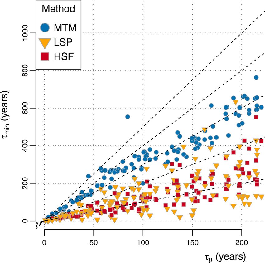
R. Hébert et al.: Scaling of palaeoclimate time series                                                                                313

Table 1. Table of acronyms used in this paper and references.

                           Acronym     Long name                             Key reference
                           CPG         Classical periodogram                 Schuster (1898)
                           LSP         Lomb–Scargle periodogram              Lomb (1976), Scargle (1982)
                           MTM         Multitaper spectrum method            Thomson (1982)
                           HSF         First-order Haar structure function   Lovejoy and Schertzer (2012)
                           DFA         Detrended fluctuations analysis       Peng et al. (1995)
                           LGM         Last Glacial maximum                  CLIMAP Project Members (1976)
                           fGn         Fractional Gaussian noise             Mandelbrot and Van Ness (1968)
                           fBm         Fractional Brownian motion            Mandelbrot and Van Ness (1968)

ment (i.e. q = 1 corresponds to the mean, q = 2 to the vari-            intermittency correction from the moment scaling function
ance, q = 3 to the skewness and so on), and ξ(q) = qH −                 K(q).
K(q) is the exponent function, where H is the fluctuation                  Under the quasi-Gaussian assumption, we can simplify
scaling exponent and K(q) is the moment scaling function.               Eq. (2) since this implies K(2) ≈ 0 and, therefore, the fol-
K(q) is zero for some monofractals such as the well-studied             lowing:
case of Gaussian processes and, thus, for these specific cases,
all statistical moments scale similarly, i.e. ξ(q) ∝ qH .               β ≈ 1 + 2H .                                                   (3)
   The equivalent metric for the power spectrum method is               This allows us to convert estimated β̂ (where ∧ denotes an es-
the spectral scaling exponent β (see Sect. 2.1.1 for a formal           timator for the given quantity) into their equivalent estimated
definition). The two scaling exponents can be related by the            fluctuation scaling exponents Ĥ . We use the fluctuation scal-
following:                                                              ing exponent H for intercomparison between the methods in
                                                                        this study. H is a natural choice as it directly describes the
β = 1 + 2H − K(2),                                              (2)     behaviour of fluctuations in real space and is the usual pa-
                                                                        rameter in functions for generating fractional noises (Man-
where K(q) at q = 2 is used since the spectrum is a second-             delbrot and Van Ness, 1968; Mandelbrot, 1971; Molz et al.,
order statistic. This relation can be understood intuitively            1997). While the fluctuation exponent H takes its origin in
since β describes the scaling of the power spectral density             the so-called Hurst exponent (Hurst, 1956), its meaning and
obtained via the Fourier transform of the auto-covariance               definition have evolved and changed over time (see Graves
function, whereas H describes the scaling of the real space             et al. (2017) and Lovejoy et al. (2021) for historical sum-
fluctuations. Therefore, since the auto-covariance is propor-           maries).
tional to the expectation value of the (zero mean) time series             The process for estimating the scaling exponents can be di-
squared, the exponent H is multiplied by two, while the in-             vided into three steps. First, if the series is irregularly spaced,
tegration in the definition of the Fourier transform increases          it requires regularization in order to be usable for the CPG
the scaling exponent by +1.                                             and the MTM. The regularization is not necessary for the
   In this work, we will focus on the (monofractal) quasi-              HSF and the LSP, which have the advantage that they can be
Gaussian case, i.e. when statistics approximately follow the            calculated directly on the irregular time series. Second, the
Gaussian distribution, in order to minimize the number of               fluctuations proper to each method are calculated as a func-
estimated parameters. Palaeoclimate archives often lack the             tion of timescale, and finally, the scaling exponent is fitted on
resolution and/or length to estimate many parameters with               the result.
confidence. This assumption is rather well justified for tem-
perature and precipitation time series at timescales longer             2.1.1   Power spectrum
than the turbulent weather regime (i.e. timescales longer
than weeks or a few years, depending on the location and                For an ergodic, weakly stationary stochastic process, the
medium; Lovejoy and Schertzer, 2012), but it is unclear over            power spectrum P of a single realization X is given by
what range of time and timescales it may hold. For a series             the Fourier transform of the auto-covariance function γ and,
on glacial–interglacial timescales comprising a Dansgaard–              equivalently, the squared Fourier transform of the signal, as
Oeschger event, multifractality has been observed (Schmitt              follows (von Storch and Zwiers, 1984):
et al., 1995; Shao and Ditlevsen, 2016), and the Gaussian ap-
                                                                                   |F{X}|2
proximation does not hold. This is also the case for highly in-         P (τ ) =           = F(γ {X}) ,                                (4)
termittent archives which clearly display multifractality, such                       T
as volcanic series (Lovejoy and Varotsos, 2016) or dust flux            where τ is the timescale, T is the temporal coverage of X,
(Lovejoy and Lambert, 2019), which would also require the               and F denotes the Fourier transform operator. Equivalently,

https://doi.org/10.5194/npg-28-311-2021                                              Nonlin. Processes Geophys., 28, 311–328, 2021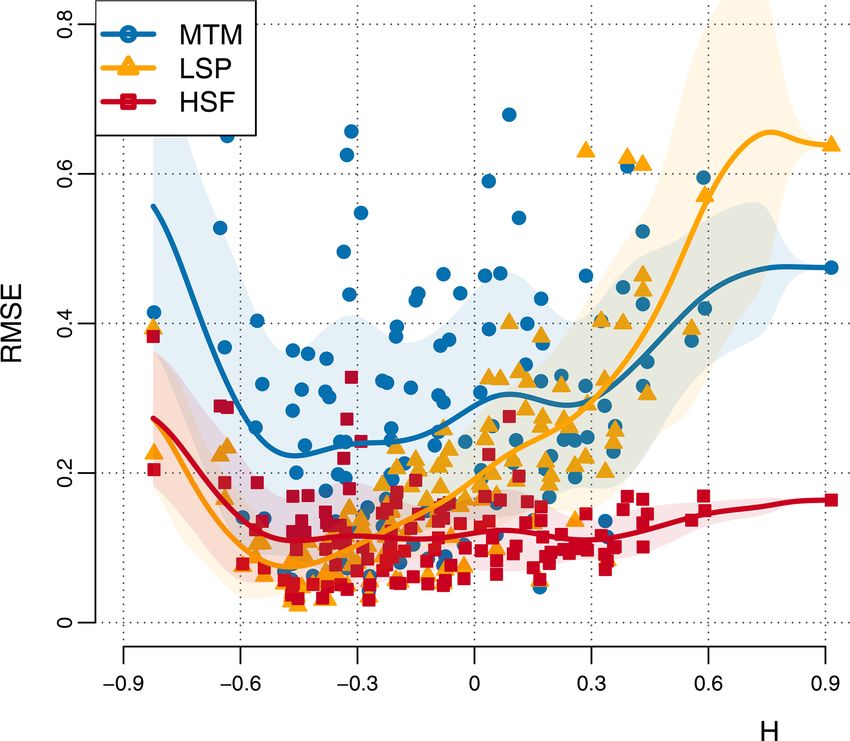
314 R. Hébert et al.: Scaling of palaeoclimate time series
the power spectrum can be given as a function of the fre- therefore, a linear interpolation multiplies the power spec-
quency f = τ −1 instead of the timescale τ . We choose to trum by sinc4 modulated by the resolution of the interpola-
write it as a function of timescale to allow for a visual com- tion (Smith, 2011), resulting in a power loss near the Nyquist
parison with the Haar method below, and also because it is frequency.
more intuitive; a non-expert can easily grasp what the 1000-
year timescale means rather than the equivalent 0.001-year−1 Lomb–Scargle periodogram
frequency.
As an alternative to the classical periodogram which requires
Classical periodogram regular data, Scargle (1982) introduced the LSP as a gener-
alized form of the CPG, as follows (Eq. 5):
The power spectrum for a discrete process X with N time "
N
#2
steps at regular intervals τ0 can be estimated using the clas- A2 X 2π(tj − T )
P̂LS (τ ) = X(tj ) cos (8)
sical periodogram as follows (Chatfield, 2013): 2 j
τ
" #2
N
N 2 B2 X 2π(tj − T )
1 X −2πiτ0 t + X(tj ) sin , (9)
P̂C (τ ) = Xt e τ . (5) 2 τ
π N t=1 j
where A, B and T are arbitrary functions of timescale τ
If log(P (τ )) behaves linearly over a range of log- and sampling
q times tj , which can be irregular. We see that,
transformed timescales log(τ ), the time series is consid-
if A = B = N2 and T = 0, we would recover the classical
ered to be power law scaling over this timescale band, i.e.
periodogram in case of regular sampling, but the reduction
P (τ ) ≈ Aτ β for an arbitrary constant A.
is not unique and other choices of A and B can be made.
Multitaper spectrum The periodogram estimates are chi-squared distributed with
2 degrees of freedom (i.e. an exponential distribution), and
The MTM method improves upon the CPG by producing in- therefore, A and B will be chosen to retain this property. For
dependent estimates using a set of orthogonal functions. The independent and identically distributed white noise, it is the
prolate spheroidal wave functions ht,k (Slepian and Pollak, case when, as in the following:
1961), also known as the Slepian tapers, have the desirable
v
uN
property of minimizing spectral leakage (Thomson, 1982).
uX 2π tj
A(τ, tj ) = t cos2 , (10)
The spectral individual estimates for the kth taper can be j
τ
written in a form similar to the periodogram above, as fol-
lows: v
uN
uX 2π νtj
N 2 B(τ, tj ) = t sin2 . (11)
1 X −2πiτ0 t
j
τ
P̂k (τ ) = hk,t Xt e τ . (6)
π N t=1
The CPG is invariant to time translation since shifting the
time steps by a constant value only affects the phase of the
The estimator can then be expressed as the mean of the K
complex exponential inside the absolute value. The function
tapered estimates as follows:
T is thus introduced for the generalized periodogram to re-
tain that property, which is the case when, as in the following:
1 K−1
X
P̂MT (τ ) = P̂k (τ ). (7) N
K k=0 P
sin 4π τ −1 t
j
τ j
T (τ, tj ) = tan−1 . (12)
Interpolation 4π PN
−1
cos 4π τ tj
j
To produce the power spectrum with the methods above, it
is necessary to interpolate the series at a regular resolution. The LSP has been mostly used in astronomy to detect pe-
Following Laepple and Huybers (2013), the data were first riodic components in noisy irregular data. As outlined above,
linearly interpolated to 10 times the mean resolution and then the functions A and B are chosen following the assumption
low-pass filtered, using a finite response filter with a cut-off that the process X is approximately white noise with no tem-
frequency of 1.2 divided by the target mean resolution in or- poral correlation. This assumption is, of course, problematic
der to avoid aliasing. Linear interpolation corresponds to a from the perspective of climate time series which usually
convolution in the temporal domain with a triangular win- exhibit long-range temporal correlations, but as we will see
dow. The Fourier transform of the triangular window is sinc2 , later, good estimates of scaling exponents can nonetheless be
where the sinc function is defined as sinc = x −1 sin(x), and recovered over a wide range of H .
Nonlin. Processes Geophys., 28, 311–328, 2021 https://doi.org/10.5194/npg-28-311-2021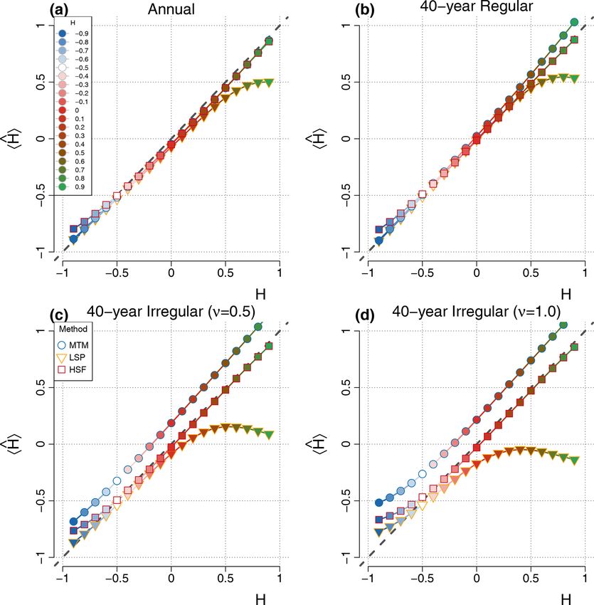
R. Hébert et al.: Scaling of palaeoclimate time series                                                                                         315

2.1.2       Haar structure function                                               2.1.3   Slope estimation

The HSF allows us to perform the scaling analysis in real                         For a power law relationship between variables x and y, such
space, i.e. without performing a Fourier transform. When                          as y = Ax B , it is usual to use standard least square fitting to
used to define a structure function, Haar wavelets are appro-                     find the coefficient A and the exponent B as the linear coef-
priate for estimating the fluctuation exponent of processes                       ficients of the equivalent linear relationship after taking the
with H ∈ (−1, 1) (Lovejoy and Schertzer, 2012), a range                           logarithm of the equation, such that log y = B log x + log A.
covering most geophysical processes. Therefore, and also be-                      Least square fitting assumes the residuals are normally dis-
cause of its readiness to be applied to irregular series and its                  tributed, which is often a good approximation for the loga-
ease of interpretation, Lovejoy and Schertzer (2012) argued                       rithm of the power spectral density of a stochastic process at
that it makes it a convenient choice for the scaling analysis                     a given frequency.
of geophysical time series.                                                          In the case of stationary Gaussian processes, it can be
   Haar fluctuations H are simple to implement for irregular                      shown that the CPG and LSP estimates at a given timescale
sampling. They can be defined for a given interval of length                      are distributed like a chi-square distribution with degrees of
τ as the difference between the mean of the first half of the                     freedom equal to 2 (i.e. an exponential distribution), and for
interval with the second half, as follows:                                        the MTM, it is approximately twice the number of tapers, al-
Hτ,j (X(ti ))                                                                     beit slightly less depending on their degree of dependence.
                                                                                  The logarithm of the distributions mentioned above is simi-
        2           X                              X
                                                                                  lar enough to a normal distribution to obtain reasonable es-
  =                                 X(ti ) −                    X(ti ) .   (13)
        τ        τ                                          τ                     timates with an ordinary least-square fit. Another option is
            tj +   < t i < tj + τ              tj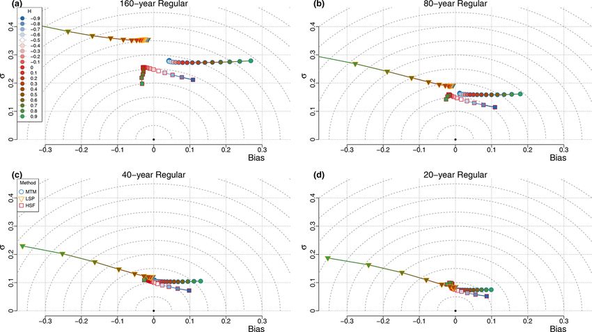
316                                                                    R. Hébert et al.: Scaling of palaeoclimate time series

Kunz et al., 2020), fitting over the small timescales produces    Generation of irregular palaeo-series
a positive bias on the slope estimation. Therefore, when es-
timating the scaling exponents for the irregular series, we       To produce irregularly sampled series akin to palaeoclimate
consistently fitted above 3 times the mean resolution τµ as       archives, an annual resolution series with a given scaling ex-
a compromise (i.e. 1.5 times the Nyquist frequency). This         ponent is first produced, with the above method, and then
choice of τmin was informed (as for the methods below) from       degraded at the desired resolution using two different meth-
the results using the palaeoclimate database (see Sect. 3.3).     ods. The first one is to simply block average, and the second
   For both the HSF and LSP, we used twice the resolution         one is to subsample a low-pass filtered version of the series.
as τmin for the regular cases, and we used τmin = 2τµ for the        For the block averaging method, boundaries are deter-
irregular cases.                                                  mined as the midpoint between subsequent time steps, and
                                                                  all data in between are averaged. This corresponds, in the
2.2     Evaluation of the estimators                              temporal domain, to a convolution with a square window,
                                                                  or, equivalently in the Fourier domain, to a multiplication
2.2.1    Surrogate data                                           of the Fourier transform with the sinc function (sinc(x) =
                                                                  x −1 sin(x)). Therefore, the power spectrum is multiplied by
                                                                  a sinc2 , and this brings about a loss of power at the high fre-
To test the methods, we produce surrogate data with the same
                                                                  quencies. For the second method, the timescale of the low-
characteristic as the palaeoclimate archives, namely a given
                                                                  pass filter is taken as twice the mean resolution of the series,
scaling behaviour and an irregular sampling in time.              and the filtered series is simply subsampled at the desired
                                                                  time steps. In the frequency domain, the filtering corresponds
Simulation of power law noise                                     to multiplying the spectrum by a square function, which cuts
                                                                  off variability below the specified timescale, and therefore,
A classical example of a non-stationary process (H > 0) is        this is useful for reducing the aliasing of higher frequencies.
normal Brownian motion (H = 21 ), which is produced by (in-          The first method would correspond to an archive sampled
teger order) integration of a normal Gaussian white noise         without gaps and where there is no smoothing of the sig-
(H = − 21 ). A process with a given scaling behaviour can         nal, for example speleothem and varved sediments, if sam-
be obtained by fractional, rather than integer, order integra-    ples containing several layers are taken or marine records
tion (or differentiation) of a given set of innovations, i.e. a   when the sample distance is smaller than the typical mix-
random series of uncorrelated values obtained from a cer-         ing depth in the sediment (Berger and Heath, 1968). The
tain distribution. To generate our surrogate data, we consider    second method would correspond to archives with spaced-
the simplest case for which the innovations are drawn from a      out sampling (for example, 1 cm every 10 cm) and including
normal Gaussian distribution. This leads to the classical frac-   processes such as bio-turbation and diffusion which smooth
tional Gaussian noise (fGn) and fractional Brownian motion        out the high-frequency signal, for example biochemical and
(fBm; Mandelbrot and Van Ness, 1968; Mandelbrot, 1971;            ecological data extracted from sediment cores (Dolman and
Molz et al., 1997). For any fGn process, there is a related       Laepple, 2018; Dolman et al., 2021). We show the second
fBm process which can be obtained by (integer order) in-          method as our main result, since it is more common to have
tegration, which increases the scaling exponent of the pro-       archives with such smoothing processes, but also because it
cess by +1. It is usual to define the associated fGn and fBm      removes most of the aliasing effect from our results. It, there-
processes by the same scaling exponent h ∈ (0, 1), which di-      fore, leaves a clearer picture of the other effects inherent to
rectly describes the scaling behaviour of the HSF for the fBm     each method. It is, however, an idealization since the smooth-
or for the fGn after (integer order) integration. However, it     ing timescale of the physical processes involved is not related
is inconvenient to use the same parameter for both fGn and        to the resolution; it should be independently estimated and
fBm when considering them in a common framework, and              accounted for in applied studies, although it is seldom re-
we prefer to also identify the fGn by the scaling behaviour       ported. All the results were also computed for the block av-
of its HSF rather than that of its integral, such that it has     erage method and are shown in the Supplement (Figs. S1–S5
H ∈ (−1, 0). In the current paper, we generally refer to both     and S7–S10).
fGn and fBm as “fractional noise” described by an exponent           Previous studies have shown that the distribution of sam-
H ∈ (−1, 1). They are generated using an algorithm devel-         pling times for typical sedimentary records can be approxi-
oped by Franzke et al. (2012).                                    mated by a gamma distribution (Reschke et al., 2019a). To
   Series with H ∈ (−0.5, −0.3) are typical of monthly land       systematically test the impact of increasingly irregular sam-
air surface temperature up to decadal timescales, while series    pling, we thus draw the time steps from a gamma distribution
with H ∈ (−0.3, 0) are more typical of sea surface tempera-       defined by its shape parameter k (or skewness ν, such that
ture over similar timescales. Non-stationary behaviour with       k = ν −1 ) and mean parameter µ which corresponds to the
H > 0 is typically observed in pre-Holocene series compris-       mean time step τµ . When the skewness parameter is ν = 0,
ing Dansgaard–Oeschger events (Nilsen et al., 2016).              then we have regular sampling of width µ. Figure 1 shows an

Nonlin. Processes Geophys., 28, 311–328, 2021                                        https://doi.org/10.5194/npg-28-311-2021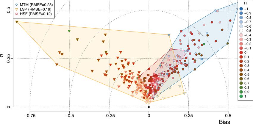
R. Hébert et al.: Scaling of palaeoclimate time series                                                                         317

example of such a surrogate series at annual resolution and        the input scaling exponents. For each method, we calculate
an irregularly degraded version (with time steps drawn from        the bias and standard deviation over the ensembles of surro-
a gamma distribution with ν = 1), along with the results of        gate data, for input H between −0.9 and 0.9 in increments of
applying the three scaling estimation methods considered for       0.1. This wide range of H values covers all values encoun-
the main analysis, i.e. the MTM, the HSF and the LSP. We           tered later in the multiproxy database; the vast majority of
omit a discussion of the results computed using the CPG as         climatic series even fall within an even more restricted range
they are generally very similar to those of the MTM, albeit        of H ∈ [−0.5, 0.5]. First, we consider the ideal case of reg-
with higher variance.                                              ular sampling, then we study the effect of irregular sampling
                                                                   and finally, the impact of the length of the time series.
2.2.2    Performance metrics and performance plots
                                                                   3.1   Effect of regular and irregular sampling
Our aim is to evaluate how the different methods perform in
the estimation of scaling exponents for irregularly sampled        We evaluate the estimators for four cases pertaining to the
palaeoclimate data X(t), with different scaling behaviour and      resolution of the data and always a fixed length of 128 data
of variable length and irregularity. In order to assess the ac-    points (Figs. 3 and 4). The first case considers annual data,
curacy and precision of our scaling exponent estimator Ĥ for      which was directly simulated and not degraded afterwards; it
a given set of parameters, we generate an ensemble of sur-         is, therefore, regular. It is shown for comparison with the sec-
rogate data X̂(t) and analyze its statistics. We evaluate three    ond case, where we simulate 5120-year-long series and then
measures, namely the bias B for the accuracy of the estima-        degrade them to 40-year resolution. This allows us to study
tor Ĥ with respect to the input H , the standard deviation σ      the impact of the degrading method, which is necessary for
for the precision of the estimator and the root mean square        producing irregular series. The third and fourth cases deal
error (RMSE), which combines both previous measures as             with series of 128 irregular time steps drawn from a gamma
follows:                                                           distribution with skewness ν = 0.5 and ν = 1, respectively,
B = hĤ i − H                                              (15)    and a mean parameter of 40 years so that the resulting series
    q                                                              have the same mean resolution as the second (regular) case.
σ = hĤ 2 i − hĤ i2                                       (16)    To illustrate the contribution of different frequency ranges to
                                                                   the precision and accuracy of the estimators, the scaling ex-
RMSE2 = B 2 + σ 2 .                                        (17)
                                                                   ponents were also fit on subranges of equal width in the log
We exploited the geometric relation between the three to eas-      of the timescales, which we refer to as the shorter timescales,
ily visualize the results. We summarize the results for a set      the intermediate timescales and the longer timescales, cor-
of parameters by one point on a bias–standard deviation di-        responding to, respectively, 2–9.2 τµ , 4.3–19.9 τµ and 9.2–
agram (Fig. 4), where the x axis gives the bias, the y axis        42.7 τµ , where τµ is the mean resolution of the time series
the standard deviation and the distance from the origin then       (Fig. 5).
corresponds to the root mean square error. The bias and stan-          For the annual data series, the scaling exponent H can gen-
dard deviation for each combination are calculated from a          erally be recovered for all values of H ∈ [−0.9, 0.9], with a
large ensemble of surrogate data (10 000 realizations).            standard deviation below 0.13 and an absolute bias less than
                                                                   0.06 (Fig. 4; top left), except for the LSP when H > −0.1, as
2.3     Data                                                       it increasingly underestimates higher values of H . The small
                                                                   bias observed in the MTM and LSP estimates stems from
In order to test the methods with the sampling properties of
                                                                   the shorter timescales (Fig. 5), which are sensitive to alias-
typical palaeo-proxy data, we consider an available database
                                                                   ing of the power below the Nyquist frequency, and, there-
of marine and terrestrial proxy records for temperature (Re-
                                                                   fore, the measured scaling slope of series with negative β
hfeld et al., 2018), which was also used for signal-to-noise
                                                                   (i.e. H < −0.5) are biased high, whereas increasingly neg-
ratio assessments by Reschke et al. (2019b). Each of the 99
                                                                   ative bias is obtained for increasingly positive values of β
sites covers at least 4000 years in the interval of the Holocene
                                                                   (H > −0.5). It follows that the flat case of β = 0 (H = −0.5)
(8–0 kyr ago; 88 time series in total) and/or the LGM (27–
                                                                   is unbiased by aliasing since the aliased power is likewise
19 kyr ago; 39 time series total) at a mean sampling inter-
                                                                   flat. The HSF-based estimates also have a significant bias in
val of 225 years or lower. These records are irregularly sam-
                                                                   the other direction when the series considered have an input
pled in time and come with different sampling characteristics
                                                                   H decreasing below H = −0.5 (Fig. 3).
(Fig. 2).
                                                                       The second case of regular 40-year series yields similar
                                                                   results to the previous case, although there is no more alias-
3     Results                                                      ing since we subsampled the 5120-year-long series at 40-
                                                                   year intervals after an 80-year low-pass filter was applied
Using the methods described above to generate synthetic            (Fig. 4; top right). The MTM returns a consistent estimate
data, we can evaluate the ability of each method to recover        with a variance which remains almost constant over the range

https://doi.org/10.5194/npg-28-311-2021                                        Nonlin. Processes Geophys., 28, 311–328, 2021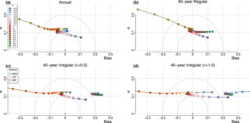
318                                                                            R. Hébert et al.: Scaling of palaeoclimate time series

Figure 1. (a, e, i, m, q, u) Surrogate time series generated with a given H are shown at annual resolution (brown), degraded to a regular
50-year resolution (blue) and degraded to an irregular and random spacing drawn out of a gamma distribution, with skewness ν = 1 and a
mean of 50 years. (b, f, j, n, r, v) Shown are the mean power spectra, estimated using the MTM of 100 realizations of surrogate time series,
generated as in the first column and shown with the same colour scheme. The irregular case is also shown after dividing the power spectra
by the expected sinc4 bias due to interpolation (dashed pink line). Also shown are the bounds for the fitting range considered later (vertical
dashed blue line) at the Nyquist frequency corresponding to 100 years, at 1.5 times the Nyquist frequency corresponding to 150 years and
at one-third of the length of the time series at 2000 years. (c, g, k, o, s, w) Same as the second column but for the LSP instead of the MTM.
(d, h, l, p, t, x) Same as the second column but showing HSF instead of MTM power spectra.

Nonlin. Processes Geophys., 28, 311–328, 2021                                                 https://doi.org/10.5194/npg-28-311-2021
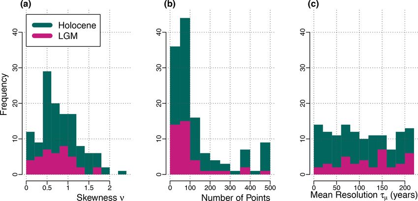
R. Hébert et al.: Scaling of palaeoclimate time series                                                                                       319

Figure 2. Sampling characteristics of the 127 palaeoclimate time series (Rehfeld et al., 2018). The 88 Holocene series (teal) and 39 Last
Glacial maximum series (pink) are evaluated along the following characteristics: (a) the skewness ν of the distribution of time steps, (b) the
number of points, i.e. samples, and (c) the mean resolution τµ of the time steps.

Figure 3. Mean estimate hĤ i from the surrogate time series with input values of H ∈ (−1, 1) (i.e. β ∈ (−1, 3)). Deviations from the one-
to-one line (dashed grey) correspond to the bias B of the mean estimate hĤ i. Different types of data are evaluated, namely (a) regular
annual data, i.e. it was directly simulated and not degraded after, (b) regular surrogate data degraded at regular 40-year intervals and irregular
surrogate data with time steps drawn from a gamma distribution with (c) skewness ν = 0.5 or (d) skewness ν = 1.

https://doi.org/10.5194/npg-28-311-2021                                                  Nonlin. Processes Geophys., 28, 311–328, 2021
320                                                                               R. Hébert et al.: Scaling of palaeoclimate time series

Figure 4. Bias–standard deviation diagram for ensembles of H estimate surrogate time series, with input values of H ∈ (−1, 1) (i.e. β ∈
(−1, 3)). Different types of data are evaluated, namely (a) regular annual data, i.e. it was directly simulated and not degraded after, (b) regular
surrogate data degraded at regular 40-year intervals and irregular surrogate data with time steps drawn from a gamma distribution with
(c) skewness ν = 0.5 or (d) skewness ν = 1.

of H . The estimator has little bias for stationary series with                The negative bias for the LSP evoked above for H > 0.5
H < 0, but it steadily increases for higher values as the lower             amplifies with irregularity and even significantly affects a
frequencies bend upward (Fig. 5). This seems to be related                  wider range of H values, down to H = −0.5 for the most
to the biased low characteristic of the MTM at the longest                  irregular case (ν = 1.). This is a consequence of higher than
timescales (Prieto et al., 2007), which creates an inflection               expected variance over the smaller timescales in the LSP
point (around 1t ≈ 3000 years on Fig. 1), and the power lost                when the slope is steep, as already identified by Schulz and
to its right appears redistributed to its left. Therefore, as H             Mudelsee (2002) using red noise. The HSF estimates, on the
increases, the amount of power lost is more important and                   other hand, remain mostly insensitive to the irregular sam-
the inflection stronger. The LSP estimates are also largely                 pling for all H > −0.5, but we already identified the positive
unbiased until about H = 0.5, and above it, a strong nega-                  bias in the regular case when H < −0.5 amplifies for more
tive bias is developed, particularly on the side of the smaller             negative values of H . Similarly, all methods yield increasing
timescales (Figs. 5, 3 and 1).                                              positive bias for such an anti-persistent time series (i.e. with
   The problem of irregularity is considered, using irregular               H < −0.5) when the sampling is irregular. This conjuncture
surrogate data skewness parameter ν = 0.5 and ν = 1 (Fig. 4;                seems to indicate that the anti-correlation characteristic of
bottom row). In the case of the MTM, we observe a consis-                   H < −0.5 processes is lost, to some extent, when degraded
tent bias for all H of about 0.5 and 0.1 for the shorter and                in an irregular manner to produce the surrogate data, as they
intermediate timescales, respectively, for the weakly irregu-               all show a similar increase of their bias (by about 0.15 for the
lar case (ν = 0.5) and practically no bias (0.02) at the longer             H = −0.9 case) with respect to their bias for the H = −0.5
timescales (Fig. 5). This corresponds very closely to the ex-               case (Figs. 3 and 4).
pected bias from the linear interpolation step, and it could
potentially be accounted and corrected for. While it is out-                3.2   Effect of time series length
side of the scope of this study to formally develop such a
method, if we apply a first-order correction by dividing the                While the irregularity had a larger impact on the bias of the
MTM spectra by a sinc4 with time constant corresponding to                  estimator, the length of the time series mostly influences the
the mean sampling resolution, we can greatly reduce the bias                variance of the estimator (Figs. 6 and S12).
down to the Nyquist frequency (Figs. 1 and S11).

Nonlin. Processes Geophys., 28, 311–328, 2021                                                    https://doi.org/10.5194/npg-28-311-2021
R. Hébert et al.: Scaling of palaeoclimate time series 321
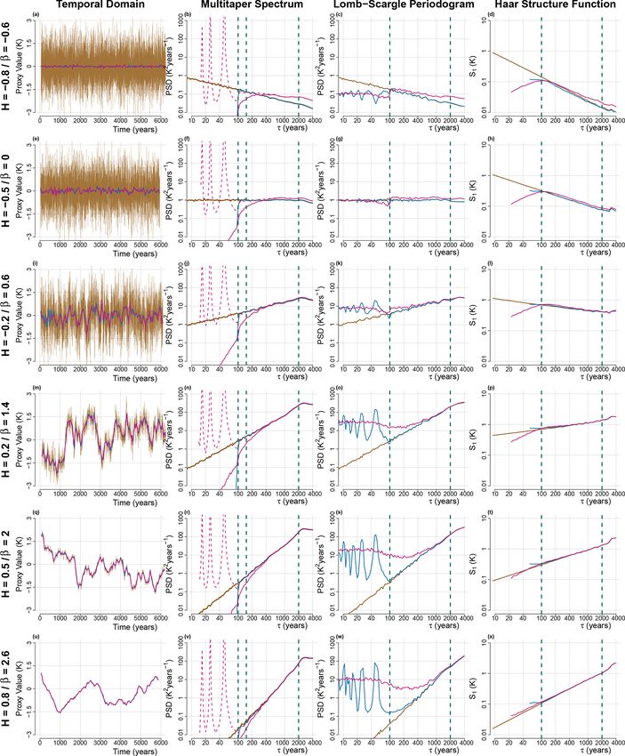
Figure 5. Timescale dependence of the bias and variance for regular and irregular series. We evaluate the following three methods: MTM
(circles), HSF (squares) and LSP (triangles). The colours correspond to the input H value for each simulation, ranging from −0.9 to 0.9
in increments of 0.1. The rows correspond to different types of surrogate series, namely (a–c) annual data, (d–f) regular data, (g–i) mildly
irregular data (ν = 0.5) and (j–l) strongly irregular data (ν = 1.0); see Sect. 2.2.1. The columns correspond to three different fitting ranges in
terms of the mean resolution τµ . (a, d, g, j) Shorter timescales – 2–9.2 τµ . (b, e, h, k) Intermediate timescales – 4.3–19.9 τµ . (c, f, i, l) Longer
timescales – 9.2–42.7 τµ .
In the case of the MTM estimates, all values of H result year resolution (Fig. S12). The bias also improves when the
in a similar standard deviation for a given resolution. When resolution increases, particularly for the higher values of H ,
the resolution is doubled, the standard
√ deviation increases by such as for H = 0.9, which goes from B ≈ 0.27 at the 160-
a factor close to the expected 2 (by ∼ 1.4–1.7), going from year resolution to B ≈ 0.10 at the 20-year resolution, while
σ ≈ 0.27 at the 160-year resolution to σ ≈ 0.07 at the 20-
https://doi.org/10.5194/npg-28-311-2021 Nonlin. Processes Geophys., 28, 311–328, 2021322 R. Hébert et al.: Scaling of palaeoclimate time series
Figure 6. The performance of the estimators is shown for regular surrogate data of different resolutions at (a) 160 years, (b) 80 years,
(c) 40 years and (d) 20 years. For each case, the series spanned 5120 years, and therefore, each case contains 32, 64, 128 and 256 data points,
respectively.
for negative H values it goes from B ≈ 0.05–0.07 to |B| < 3.3 Application to database
0.01 for the same resolution change (Figs. 6 and S6).
In the case of the LSP, up to H ≈ 0.1, the standard devi-
√ In order to see how these results translate to typical proxy
ation of the estimates also decrease by a factor close to 2 records, we perform the analysis with surrogate data with
(by ∼ 1.4–1.8; Fig. S12) with each doubling of resolution, sampling characteristic and scaling behaviour directly ex-
going from σ ≈ 0.35 at the 160-year resolution to σ ≈ 0.08 tracted from the database of Holocene and LGM records (see
at the 20-year resolution, and the bias improves only slightly Sect. 2.3). We make the assumption that the series approxi-
since it was already small (|B| < 0.04). For the higher H mately follow power law scaling, and that they can, therefore,
values, the standard deviation improves less (by ∼ 1.2–1.4 be modelled by fractional noise described by a scaling expo-
at H = 0.9; Fig. S12), going from σ ≈ 0.43 at the 160-year nent H . Since the best H to describe the approximate scal-
resolution to only σ ≈ 0.19 at the 20-year resolution. At the ing behaviour of the series is unknown, we make an initial
same time, the bias change becomes more positive, thus com- approximation with each method and take the median of the
pensating slightly better for the overall strong negative bias three results as the reference value for the given series, with
characteristic of the LSP estimates for very high H values. which we generate an ensemble of surrogates with the same
In the case of the HSF, when increasing the resolution, the sampling scheme as the given series. We use the real time
standard deviation of the estimates improves more for the steps in order to evaluate the impact of each specific sam-
lower H values than for the higher values, improving by a pling scheme. Again, we consistently fitted up to one-third
factor of ∼ 1.4–1.8 for H = −0.9 to ∼ 1.2–1.4 for H = 0.9 of the length (see Sect. 2.1.3) but empirically determined the
(Fig. S12). Overall, the standard deviation improves from best minimum fitting scale τmin such that it minimizes the
σ ≈ 0.20–0.25 at the 160-year resolution to σ ≈ 0.06–0.09 RMSE of the estimator with respect to the reference H used
at the 20-year resolution. The slight negative bias found for to generate the surrogate data.
the H > −0.5 estimates (|B| < 0.04) practically vanishes but We found the HSF to yield the smallest τmin of the three
not the positive one for H < −0.5, which only decreases methods, with τmin below twice the value of the mean reso-
slightly. lution τµ for 121 out of 127 series and even below τµ for 43
out of 127 (Fig. 7). The LSP yielded similar results, with 109
out of 127 series having τmin below twice the value of τµ and
Nonlin. Processes Geophys., 28, 311–328, 2021 https://doi.org/10.5194/npg-28-311-2021R. Hébert et al.: Scaling of palaeoclimate time series 323
4 Discussion
Our comparative study indicates that, for irregular time se-
ries, the methods with interpolation, i.e. the CPG and the
MTM, are less efficient for evaluating variability across
timescales than the methods without interpolation, i.e. the
LSP and the HSF. In the case of regular time series, however,
all methods were found to perform similarly (Fig. 4b) for a
wide range of input H and only showed bias on the fringes
of the H range considered. In addition, we found that the
choice of method should also be informed by the character-
istics of the underlying process measured since there was an
observed dependence between the performance metrics and
the scaling exponent H which generated the surrogate data.
As such, the LSP may only be appropriate for irregular series
suspected of having H near or below H = −0.5, while the
HSF shows better reliability even when H is near or above
H = 0. It might not be so surprising that the LSP performed
poorly for higher H values since it has been developed to
approximate the CPG for stationary noise processes (Scar-
Figure 7. The best minimum fitting timescales τmin (minimizing gle, 1982), and processes with H > 0 are non-stationary, i.e.
the RMSE in H ) are shown for each method as a function of the their mean is not stable and changes with time.
mean resolution τµ for ensembles of surrogate data generated with
In addition to the irregularity, we also compared how the
the same sampling scheme as the corresponding palaeoclimate time
resolution of the time series affects the estimators of H .
series from the database.
While making the series more irregular mostly affected the
accuracy of the estimates, i.e. their bias, without affecting
their precision, i.e. their standard deviation, increasing the
resolution mostly improved the precision and the accuracy
only to a lesser extent. Increasing the resolution naturally im-
41 out of 127 having τmin even lower than τµ . This contrasts proves the estimates as it provides more information and also
with the MTM, which almost never suggests best results for because it decreases the relative weight of the most uncer-
τmin below twice the value of τµ but rather an average mini- tain timescales, i.e. the smaller timescales, near the sampling
mum resolution τ min = 3.3 τµ , compared to τ min = 1.2 τµ for resolution, and the longer timescales, near the length of the
the HSF and τ min = 1.3 τµ for the LSP. This underlines the series.
point that, because interpolation-free methods give more re- Our conclusions, however, rely on the real data having
liable estimates at shorter timescales, they allow for a better similar properties to the surrogate data used to validate the
usage of the full data. methods, and the conclusions may be different if the real
The HSF yields the best results of all three methods, both data have properties different than the assumed power law
in terms of variance of the estimates and in terms of bias, scaling. It is difficult to say, for example, which method
with a mild tendency towards positive biases. The MTM also would perform best if the data analyzed contained two differ-
tends to show positive biases, albeit higher, while the LSP ent scaling regimes, i.e. one with low H and the other with
tends to show negative biases. Both the MTM and the LSP high H (Lovejoy and Schertzer, 2013). Another limitation of
generally show a higher variance of their estimators than the our surrogate data is that it is Gaussian distributed, whereas
HSF (Fig. 8), although for different reasons. The MTM has a real palaeoclimate data can exhibit multifractality (Schmitt
higher variance because the higher τmin does not allow us to et al., 1995; Shao and Ditlevsen, 2016). Furthermore, in or-
use the smaller timescales in the estimation procedure, while der to degrade the simulated annual time series into irregu-
the LSP shows higher variance because of the time series lar palaeoclimate-like data, we had to use simplified numer-
with high input H for which it performs poorly, especially ical methods to mimic the physical processes and manipula-
when the data are irregular (Fig. 4). tions leading to the recording and retrieval of palaeoclimate
On average, the HSF method gave the lowest RMSE = archives. For our purpose, we chose to low-pass filter the data
0.11 ± 0.04 compared to RMSE = 0.30 ± 0.15 and RMSE = and subsample, since this is very common in sedimentary
0.19±0.15 for the MTM and the LSP, respectively. The poor data and ice cores because of, respectively, bio-turbation and
performance of the LSP compared to the HSF stems from the diffusion (Dolman and Laepple, 2018; Dolman et al., 2021;
higher H , since it performs as well as the Haar when H < 0, Kunz et al., 2020). However, reality is more complex, and
with RMSE = 0.12 ± 0.07 (Fig. 9). other processes could significantly alter the recorded signal
https://doi.org/10.5194/npg-28-311-2021 Nonlin. Processes Geophys., 28, 311–328, 2021324 R. Hébert et al.: Scaling of palaeoclimate time series
Figure 8. Bias–standard deviation diagram for the surrogate time series generated using time steps from the palaeoclimate database. The
input H , used to generate the time series, is indicated by the colour inside the markers. The shaded polygons contain all the points for a given
method (see the legend for colours).
In summary, it is difficult to ascertain which method is the
best since the answer depends on the irregularity, the res-
olution and, most importantly, the underlying H values. In
this respect, the HSF is possibly the safer method for palaeo-
climate applications since it only performs poorly for series
with H < −0.5, an almost unseen behaviour in climatic time
series at timescales longer than decadal. Although the LSP
gives equally good results for H /0 and even better near
H = −0.5, i.e. white noise, its increasing bias and standard
deviation for higher H values makes it an uncertain choice
for timescales longer than centennial timescales since cli-
mate time series at those timescales often show values of
H ≈ 0 and greater. The MTM produces good estimates for
relatively regular series but struggles with highly irregular
time series, since it must rely on interpolation. While this
produces a large bias on the shorter timescales which we
have thus discarded, the bias is rather consistent, and meth-
ods could be developed to correct for it (e.g. Fig. S11). On
Figure 9. RMSE of the H estimates as a function of the input H for
the other hand, the longer timescales of the MTM are rel-
the surrogate time series based on the proxy database. The RMSEs
are given for the three estimation methods as a function of the H atively well estimated, and it is appropriate to estimate the
used to generate the surrogates. Also shown is a Gaussian smooth- absolute variance over a timescale band well above the mean
ing of the points for each method (thick line) and the 1 standard resolution (Rehfeld et al., 2018; Hébert et al., 2021). Fur-
deviation confidence interval (shaded). thermore, the effect of proxy biases are well studied for the
power spectrum (Kunz et al., 2020; Dolman et al., 2021),
mainly due to the known properties of the Fourier transform.
However, the MTM, and the LSP, do not allow for the charac-
and bias the variability estimates in ways not accounted for terization of intermittency through the study of all statistical
by our surrogate model. For specific case studies, it is advis- moments; this is in contrast to the HSF, which is, thus, better
able to develop forward models (Stevenson et al., 2013; Dee suited for the analysis of time series displaying multifractal-
et al., 2017; Dolman and Laepple, 2018; Casado et al., 2020) ity, such as palaeoclimate time series at glacial–interglacial
of the studied palaeoclimate archives in order to understand timescales comprising Dansgaard–Oeschger events (Schmitt
potential biases generated by the recording and specific sam- et al., 1995; Shao and Ditlevsen, 2016)
pling.
Nonlin. Processes Geophys., 28, 311–328, 2021 https://doi.org/10.5194/npg-28-311-2021R. Hébert et al.: Scaling of palaeoclimate time series 325
Our study is not comprehensive, and other methods such indeed showed the Haar structure function to give more reli-
as the bias-corrected version of Lomb–Scargle (Schulz and able estimates over a wide range of H . Given that we cannot
Mudelsee, 2002, REDFIT) and the z transform wavelet (Zhu know a priori what kind of scaling behaviour is contained in
et al., 2019) exist. More precise estimates of the scaling ex- a palaeoclimate time series, and that it is also possible that
ponent are obtained by parametric methods based on max- this changes as a function of timescale, it is a desirable char-
imum likelihood, but they require strong assumptions about acteristic for the method to handle both stationary and non-
the underlying process (Del Rio Amador and Lovejoy, 2019). stationary cases alike.
We aimed to cover the most commonly used methods that
also allow for a simple interpretation of variability across
timescales, either because they represent the well-studied Code and data availability. The data are available as the supple-
power spectrum or the Haar fluctuations directly provide ment to Rehfeld et al. (2018, https://doi.org/10.1038/nature25454)
changes in amplitude. and the code is publicly available on Zenodo (Hébert, 2021,
https://doi.org/10.5281/zenodo.5037581).
5 Conclusions
Supplement. The supplement related to this article is available on-
line at: https://doi.org/10.5194/npg-28-311-2021-supplement.
Characterizing the variability across timescales is important
for understanding the underlying dynamics of the Earth sys-
tem. It remains challenging to do so from palaeoclimate Author contributions. All authors participated in the conceptualiza-
archives, since they are more often than not irregular, and tion of the research and the methodology. RH developed the soft-
traditional methods for producing timescale-dependent esti- ware and visualization and conducted the formal analysis and inves-
mates of variability, such as the classical periodogram and tigation. KR and TL provided supervision. RH prepared the original
the multitaper spectrum, generally require regular time sam- draft, and all authors contributed to reviewing and editing the final
pling. paper.
We have compared those traditional methods using inter-
polation with interpolation-free methods, namely the Lomb–
Scargle periodogram and the first-order Haar structure func- Competing interests. The authors declare that they have no conflict
tion. The ability of those methods to produce timescale- of interest.
dependent estimates of variability when applied to irregular
data was evaluated in a comparative framework. The metric
we chose to compare them is the scaling exponent, i.e. the Disclaimer. Publisher’s note: Copernicus Publications remains
linear slope in log-transformed coordinates, since it summa- neutral with regard to jurisdictional claims in published maps and
institutional affiliations.
rizes the behaviour of the variability over a given timescale
band. Doing so assumes power law scaling, a behaviour
which is often observed in geophysical time series, at least
Special issue statement. This article is part of the special issue “A
approximatively (Mandelbrot and Wallis, 1968; Cannon and century of Milankovic’s theory of climate changes: achievements
Mandelbrot, 1984; Pelletier and Turcotte, 1999; Malamud and challenges (NPG/CP inter-journal SI)”. It is not associated with
and Turcotte, 1999; Fedi, 2016; Corral and González, 2019). a conference.
To evaluate our estimators, we generated fractional noise as
surrogate annual time series characterized by a given scal-
ing exponent H , also known as fractional Gaussian noise Acknowledgements. This study was undertaken by members of Cli-
when they are stationary (H < 0) and fractional Brownian mate Variability Across Scales (CVAS), following discussions at
motion when they are non-stationary (H > 0). The annual several workshops. CVAS is a working group of the Past Global
time series were then degraded to resolution characteristics Changes (PAGES) project, which, in turn, received support from the
of palaeoclimate archives for the recent Holocene. Swiss Academy of Sciences and the Chinese Academy of Sciences.
We found that, for scaling estimates in irregular time se- We particularly thank Torben Kunz and Shaun Lovejoy, for the
ries, the interpolation-free methods are to be preferred over in-depth discussions, and Timothy Graves and Christian Franzke,
for freely sharing the software for generating fractional noise. We
the methods requiring interpolation as they allow for the
also acknowledge discussions with Mathieu Casado, Lenin del Rio
utilization of the information from shorter timescales with- Amador, Andrew Dolman, Igor Kröner and Thomas Münch. We
out introducing additional bias. In addition, our results sug- thank all the original data contributors who made their proxy data
gest that the Haar structure function is the safer choice available. This is a contribution to the SPACE and GLACIAL
of interpolation-free method, since the Lomb–Scargle peri- LEGACY ERC projects.
odogram is unreliable when the underlying process gener-
ating the time series is not stationary. This conclusion was
reinforced by the application to the proxy database which
https://doi.org/10.5194/npg-28-311-2021 Nonlin. Processes Geophys., 28, 311–328, 2021You can also read