Context-specific volume-delay curves by combining crowd-sourced tra ic data with Automated Tra ic Counters (ATC): a case study for London

Data-Centric Engineering (2020), xx:xx 1–25
 doi:10.1017/xxxx

 R E S EARCH ARTICLE

 Context-specific volume-delay curves by combining crowd-
 sourced traffic data with Automated Traffic Counters (ATC):
arXiv:2011.01964v1 [stat.AP] 3 Nov 2020

 a case study for London
 Gerard Casey1* , Bingyu Zhao2 , Krishna Kumar3 and Kenichi Soga2
 1 Arup,London, UK. 2 Department of Civil and Environmental Engineering, University of California, Berkeley, USA.
 3 Departmentof Civil, Architectural and Environmental Engineering, University of Texas at Austin, USA.
 *Corresponding author. E-mail: gerard.casey@arup.com

 (Received xx xxx xxxx)

 Keywords: Traffic analysis, crowd-sourced data, real-time traffic data, sensors, GPS, statistical modelling

 Abstract
 Traffic congestion across the world has reached chronic levels. Despite many technological disruptions, one of the
 most fundamental and widely used functions within traffic modelling, the volume delay function, has seen little in
 the way of change since it was developed in the 1960’s. Traditionally macroscopic methods have been employed
 to relate traffic volume to vehicular journey time. The general nature of these functions enables their ease of
 use and gives widespread applicability. However, they lack the ability to consider individual road characteristics
 (i.e. geometry, presence of traffic furniture, road quality and surrounding environment). This research investigates
 the feasibility to reconstruct the model using two different data sources, namely the traffic speed from Google
 Maps’ Directions Application Programming Interface (API) and traffic volume data from automated traffic coun-
 ters (ATC). Google’s traffic speed data are crowd-sourced from the smartphone Global Positioning System (GPS)
 of road users, able to reflect real-time, context-specific traffic condition of a road. On the other hand, the ATCs
 enable the harvesting of the vehicle volume data over equally fine temporal resolutions (hourly or less). By combin-
 ing them for different road types in London, new context-specific volume-delay functions can be generated. This
 method shows promise in selected locations with the generation of robust functions. In other locations it highlights
 the need to better understand other influencing factors, such as the presence of on road parking or weather events.

 Impact Statement
 Volume delay curves are widely used in traffic analysis. They form a critical part of the traffic assignment
 stage in the four-step modelling approach. We propose a novel data-driven approach to accurately represent
 the traffic behaviour under congestion using emerging data sources for a better understanding of real-world
 context-specific behaviour.

 1. Introduction
 When the vehicular demand for a road exceeds its free-flow threshold, a journey time-delay is incurred,
 resulting in congestion. Historically in traffic studies and planning, the relationship between traffic vol-
 ume and time-delay has been simplified to macroscopic principles ignoring the behaviour of individual
 vehicles (van Wageningen-Kessels et al., 2015). The most widely adopted functional representation of
 such a macroscopic volume-delay relationship is the Bureau of Public Roads (BPR) relationship pro-
 posed in the 1960s (Bureau of Public Roads, 1964). Since then, local traffic agencies worldwide have
 © Cambridge University Press 2019. This is an Open Access article, distributed under the terms of the Creative Commons Attribution licence (http://
 creativecommons.org/licenses/by/4.0/), which permits unrestricted re-use, distribution, and reproduction in any medium, provided the original work
 is properly cited.

2 Gerard Casey et al.

calibrated the BPR curve coefficients to suit the local needs, such as in Suh et al. (1990); Kurth et al.
(1996); Irawan et al. (2010); Mtoi and Moses (2014); Kucharski and Drabicki (2017). However, the
calibration of BPR coefficients to local roads requires an extensive set of volume and delay data, and
gathering such data (e.g., through surveys) is often a challenge. Hence, traffic engineers often end up
using a generic set of coefficients to cover a wide range of roads (for example, one set of coefficients
for all roads in the city, without considering the presence of road furniture or on-street parking that
could affect the road capacity) and do not updated these coefficients to the changing demands of the
city. Nevertheless, real-world conditions exhibit an enormous variability in the volume-delay charac-
teristics, which is nearly impossible to account for entirely and certainly insufficient when representing
this volume-delay relationship using a generic and static function for the entire city. Therefore, it is
critical to understand the errors in volume-delay prediction based on real-world data.
 This research aims to provide an efficient data-driven approach to calibrating the volume-delay
curves by incorporating emerging data sources, mainly crowd-sourced travel time information from
location and routing service providers, such as Google Maps (Google Inc., 2020). This type of calibra-
tion has never been done before to our knowledge. Specifically, this paper investigates the integration
of two disparate data sources for this purpose: (1) the traffic speed data from Google Maps, and (2) the
traffic count data from the Automated Traffic Counter (ATC) system in Greater London. The reason
to combine the two data sources is two-fold: (1) first of all, many traffic detectors in cities are single
loop detectors, which do not offer accurate speed/delay measurement (Wang and Nihan, 2003); (2) sec-
ondly, even if there are speed sensors (e.g., double loop detectors or radars), they often only measure
point speeds, which do not reflect the delay experienced on the road network, especially in urban set-
tings (Wang and Liu, 2005; Zhang et al., 2015). In this study, we assess the feasibility and performance
of obtaining site-specific volume-delay information based on these new data sources.
 The paper is structured in the following way. Section 2 discusses relevant literature, including various
functional forms of the volume-delay relationships, as well as some applications of such relationships
in transport research and planning. Next, in Sections 3 and 4, we introduce the two data sources, namely
the hourly traffic volume from the ATCs and the traffic speed from Google Maps. These data are used
for estimating the road characteristics (free-flow travel time and capacity) and calibrating the volume-
delay curve coefficients. Sections 5 and 6 explain the process of data cleaning and model building.
In particular, three models are tested, including one base model with default volume-delay parameter
values and two data-informed models with partial or full set of parameters calibrated from the real-
world data. The three models are compared in terms of their performances in quantifying the level of
delays at different traffic congestion levels. Section 7 offers an extensive discussion on the potential
factors that could cause the variability observed in the volume-delay relationship, as well as the future
prospects to adopt the proposed method at larger scales. Using fine-resolution data in the form of ATCs
and aggregated device-based location-informed journey times on a range of roads, we demonstrate the
capability of the new data-driven approach for efficiently capturing the volume-delay characteristics of
roads in selected roads in Greater London.

2. Literature review
Volume-delay functions, as the name indicates, relate two fundamental traffic parameters using non-
linear mathematical expressions. The independent parameter, volume, expresses the level of traffic
demand and the dependent parameter, delay, indicates the deterioration in the traffic speed as the
demand increases. The actual trend between volume and delay is a property of the road and is related
to factors such as the speed limit, width, geometry, and the presence of road furniture. Even though
the volume-delay relationships are highly context-specific, there exist some widely accepted functional
forms to model them. The most widely used function is the BPR curve, which was developed in the

Data-Centric Engineering 3

1950s for uncongested freeways in the US. Its simple mathematical form and minimal input require-
ments are attributed to its widespread adoption (Skabardonis and Dowling, 1997). The travel time on
a road link computed using the BPR function has the form:
 
 = 0 × (1 + ( ) ) (1)
 
where 0 is the time required to traverse the road link at free-flow speed; is the road capacity (vehicles
per unit time); and are calibration coefficients; is the traffic volume to be modelled. The function
is sometimes also expressed in terms of the vehicle speed , which can be obtained from and the road
length .
 Since the BPR function was created by fitting a polynomial equation to uncongested freeway
data from the 1950s in the US, it does not reflect the current operating conditions of the road net-
work (Skabardonis and Dowling, 1997). As a result, many different organisations have adapted the BPR
curve with various local empirical and simulated data to suit the local road conditions better (Irawan
et al., 2010; Mtoi and Moses, 2014). The work of Kurth et al. (1996) focuses on obtaining refined,
free-flow time and capacity ( 0 and ) for each road based on guidelines from the Highway Capacity
Manual (HCM, 1994 version), rather than getting 0 and from traditional lookup tables with only
a few categories. Their approach is found to produce more accurate traffic speed estimations. How-
ever, it requires time-consuming identification of road characteristics (e.g., road grade, vehicle mix and
land use) and is still limited by the available adjustment factors that the HCM procedure can take into
account.
 Kucharski and Drabicki (2017) estimated both the calibration coefficients , and the road char-
acteristics 0 , together based on loop detector data. They suggested transforming the volume-delay
relationship to speed-density relationship for regression, as the latter remains monotonic in congested
cases. However, the analysis lacks rigour due to employing linear R-squared metric to quantify errors
in a non-linear model and inconsistency in calculating the density. In the case of London, Transport
for London (TfL) has calibrated the BPR function using observed traffic counts and defined = 1.0
and = 2.0 for the area (TfL, 2010). In general, these calibrated volume-delay functions fit the local
observations better.
 Apart from the BPR function, several volume-delay relationships have been proposed over the years,
as summarised in Mtoi and Moses (2014). Davidson (1966) proposed a general-purpose travel-time for-
mula in 1966 and this method has undergone numerous modifications since it was first proposed (Mtoi
and Moses, 2014). It has exhibited a closer match to actual volume counts and has a more robust theoret-
ical base than the BPR (Rose et al., 1989). Among the modifications of the Davidson function (Tisato,
1991; Akçelik, 1991), the Akçelik function is the most widely used. The Akçelik method is a time-
dependent modification of the Davidson model, which uses the coordinate transformation technique
in an attempt to overcome the conceptual and calibration issues with the Davidson method (Akçelik,
1991). This function showed good results for certain road types, tolls roads and signalized arteri-
als (Mtoi and Moses, 2014). Spiess (1990) proposed the conical method, which attempts to overcome
some of the limitations of BPR at both the upper and lower bounds by employing hyperbolic conical
sections, while maintaining a similar form to the BPR. The similarity to BPR enables a direct transfer
of parameters. These alternative formulations have also been adopted in practice and research.
 Volume-delay functions are typically employed in utility estimation (e.g., time cost) for static or
semi-dynamic traffic assignments, and informing route choices for agent-based modeling (Çolak et al.,
2016; Suh et al., 1990). The differentiable form and convex nature of volume-delay functions make
them an ideal candidate for optimisation-based traffic assignment, such as the assignment that satisfies
the Wardrop’s equilibrium (Lien et al., 2016). Despite their extensive use in research and practice, the
volume-delay functions have several limitations. For example, it is possible to obtain traffic volume-to-
capacity ratio much higher than one, which is unrealistic (Nie et al., 2004; Chiu et al., 2011). Closely
associated is the problem that the volume-delay functions can only model the hypocritical section of the
traffic fundamental diagram (monotonic increase in the flow on a link with travel time and density), but

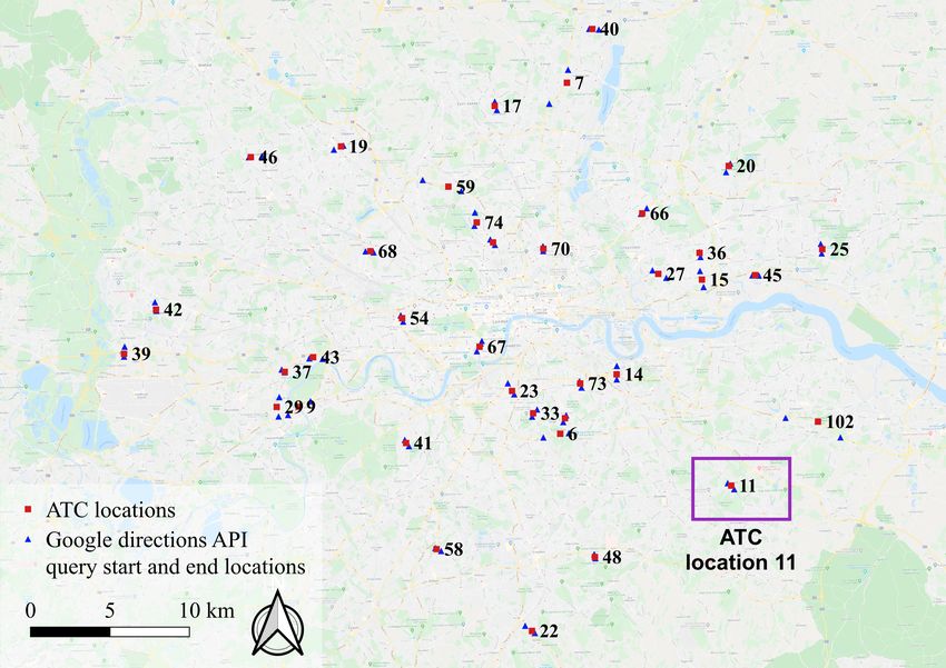
4 Gerard Casey et al.

not the hypercritical section (when a road is congested to a certain level, the flow will decrease despite
an increase in density and travel time). These limitations mean that volume-delay functions cannot
model traffic phenomena such as spillbacks, wave propagation, and gridlocks, which would require the
use of a dynamic model (Lo and Szeto, 2005; Chiu et al., 2011). These concerns are also reflected in
the UK Department for Transport (DfT) Transport Analysis Guidance (TAG), which recommended to
model junction delays explicitly especially for congested urban roads (DfT, 2020). Despite these short-
comings, volume-delay functions are a useful tool for regional-scale simulations and analysis requiring
faster computations. Carefully calibrated volume-relationships frequently show good match with the
real-world data (Kurth et al., 1996; Irawan et al., 2010).
 In order to effectively use volume-delay functions in regional-scale analyses, it is crucial to maintain
an up-to-date coefficients specific to local regions, which has proven to be a nontrivial task. Past studies
have identified the need to inform these functions with empirical and context-specific data (Rose et al.,
1989; Spiess, 1990), but also recognise the difficulty and cost associated with collecting such empirical
data as being prohibitive (Rose et al., 1989). There have been studies that incorporate different forms of
field sensor data for such calibration (Mtoi and Moses, 2014; Neuhold and Fellendorf, 2014; Kucharski
and Drabicki, 2017). Nevertheless, the data used in these studies have been generated specifically for
that application and requires specific hardware and software for use.
 Recent innovations in the information and communication technologies have led to an increase in
the adoption of real-time crowd-sourced data feeds in transport modelling. This includes applications
of location data for emissions estimations (Hirschmann et al., 2010), building origin and destination
matrices (Toole et al., 2015) and general urban traffic management applications (Artikis et al., 2014).
This study investigates the use of a novel real-time crowd-sourced data feeds that have wider spatial
coverage and are not generated specifically for estimating volume-delay functions. These sources could
be used to consider some of these previously ignored characteristics and create temporally and spatially
dynamic volume, speed and saturation relationships. Such data sources can harvest data at a finer reso-
lution over a longer (even indefinite) period of time giving a far greater understanding of the temporal
variations and trends exhibited on road infrastructure.
 This work attempts to combine new data sources in order to create functions that do not require a
large range of survey inputs. The general and transparent methodology of harvesting crowd-sourced
data enables its easy deployment to multiple sites. As a result, highly localised relationships can be
obtained for a diverse range of road links, reflecting individual characteristics of the road (i.e. geometry,
the presence of traffic furniture, road quality and the surrounding land use). Such varying characteristics
can result in very different vehicular behaviour on roads that may be considered similar by traditional
approaches.

3. Traffic volume inputs: ATCs
Two sources of data inputs are utilised to calibrate the volume-delay characteristics localised to the road
link level: the link-level traffic counts (volume) from the ATCs and the link-level travel time (delay)
from Google Maps’ real-time information. Data from these two sources were harvested over the same
time period (late February to mid March, 2016) and then paired according to the time of collection to
create volume-delay observations. These observations will be used later in this paper to calibrate the
context-specific volume-delay functions for road links where observations are available. In this and the
next section, the two data sources will be introduce.
 ATCs are magnetic induction loops embedded under the road surface. The passing of a vehicle
results in an electromagnetic signal. The ATCs in Greater London count every vehicle which passes
over the inductions loop. The data used here was harvested over a period of three weeks from the 27th
February to the 21st March 2016.
 There are 37 DfT ATC locations distributed in Greater London (Fig. 1). Among these data collecting
locations, 34 roads have ATCs operate in both directions, while three roads have ATCs operate only

Data-Centric Engineering 5

in one direction. The ATC locations provide traffic counting information for a range of different DfT
defined road classes (Table 1). The DfT (DfT, 2012a) publishes guidance on the road classification
system in the UK.

Table 1. ATC locations by road class

 Road class Trunk (Motorway or A) Principal (A) B C Unclassified Total

 Count 6 16 3 3 9 37

Figure 1. ATC Locations in Greater London (Google Inc., 2020). The red dots illustrate the locations of the ATC. The blue triangles
illustrate the origin and destination locations specified in order to harvest journey time information..

 The raw ATC data contains individual records for each vehicle that passed the counter, including
its speed and the exact time (accurate to the second). Over the test period of three weeks, there were
approximately 4.5 million recorded vehicles. An example record of a vehicle crossing the ATC Site 11
(labelled in Fig. 1) on the first day of data collection reads:
 Site: 11, Direction: Northbound, Date: 2016-02-27, Time: 00:00:28, Speed: 37.
Individual vehicle records at each ATCs are aggregated by the hour to obtain the traffic volumes per
hour (i.e., the hourly traffic flow). The total number of vehicles passing in an hour is considered as the
hourly traffic volume at the measurement site. For gathering the aggregate data at each ATC, a unique
identifier is defined by concatenating the location ID and the directionality of the ATC. For example,
the northbound detector at ATC location 11 is identified as site “11N". The timestamp is then rounded
up to the next hour in order to quantify the hourly traffic volume up to that hour. This results in an
output dataset which features traffic counts per hour for each site, along with the direction and date. A
sample of the aggregated dataset at ATC location 11N is shown in Table 2.
 Fig. 2 shows an illustration of the variations in the hourly traffic volume at ATC location 11 (north-
bound and southbound). Location 11 is situated on the Royal Parade road (A208) with the northbound
direction leading to central London and the southbound direction leaving from central London. It is
clear that during weekdays (March 7th - 11th, 2016), the northbound direction exhibits a higher peak

6 Gerard Casey et al.

Table 2. Processed ATC data record sample

 Combined ID ATC ID Direction Date Hour Hourly Traffic Volume

 11N 11 Northbound 2016-03-07 6 152
 11N 11 Northbound 2016-03-07 7 420
 11N 11 Northbound 2016-03-07 8 694
 11N 11 Northbound 2016-03-07 9 496

during the morning rush hours (commuting trips into the city), while the southbound direction carries
more traffic leaving the city during the evening peak. On weekends (March 12th and 13th, 2016), there
is only one peak, which also starts later than the regular morning peak observed on weekdays. This vari-
ation in traffic volume follows the general understanding of the distribution of traffic loads throughout
the day.

Figure 2. Hourly traffic volume distribution for Site 11 (March 7th-13th, 2016).

4. Traffic speed and time delay from Google Maps API
Link travel time, or equivalently the inverse of the space-mean speed of vehicles passing through the
link, can be collected using several methods. For example, the ATC data presented in the previous
section have vehicle speed records. However, the ATC speed is a point measurement and may not be
suitable to calculate the average travel time across the road link, as required by many traffic simulation
studies. An alternative method to infer the travel time across the link is to use real-time, crowd-sourced
location information gathered from mobile phone users. Mobile phones with location service enable
harvesting of fine resolution temporal and spatial position data obtained from GPS positioning, cell
tower triangulation, WiFi Service Set Identifier (SSID) mapping, Bluetooth, and other technologies,
either in isolation or in tandem. Such data hold a great deal of promise due to the range of possible
uses it has in the transportation sector, such as understanding peak hour travel demands and inferring
transport modes (Çolak et al., 2016; Zheng et al., 2010).
 Anonymised crowd-sourced location data is useful for understanding real-time road traffic condi-
tions on congested or smooth flowing roads (Barth, 2009). Crowd-source data collection is suitable
for urban areas with high population density, high travel demand, and high mobile phone uptake. This
information has been widely used by technology companies such as Google and Apple to inform their

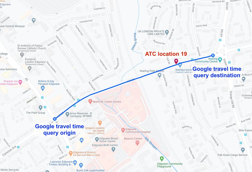
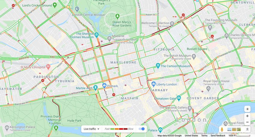
Data-Centric Engineering 7

users of the optimum path that avoids traffic (Apple Inc., 2020; Microsoft, 2020; Google Inc., 2020;
TomTom N.V., 2020). Individuals with access to these services can make an informed decision on route
choice for a given mode or even a mode decision on how to get from their starting point to a desired des-
tination with the lowest time cost. For example, Google provides real-time colour-coded maps that offer
a qualitative representation of the current traffic conditions on roads where sufficient data is available.
Figure 3 shows the traffic conditions from Google Maps traffic layer of the Camden area in London on
a typical Friday evening.

Figure 3. Google Maps Traffic Layer, showing live traffic in the Camden/Soho/Marylebone/Mayfair area of London on a Friday
evening (Google Inc., 2020).

 In this research, the traffic condition information is retrieved in batches using the Google Maps
Directions Application Programming Interface (API) (Google Cloud, 2020). Depending on the personal
settings of a mobile phone user, the freely available Google Maps app send anonymised data of their
location to Google. Such data are personally and commercially sensitive, so post-processing is carried
out by Google in order to ensure that no user movements can be isolated from the flows. Google’s
Directions API used in this paper is a service that calculates travel time and routing directions between
given origins and destinations using a Hypertext Transfer Protocol (HTTP) request (Google Cloud,
2020). The use of an HTTP request allows for scheduled and bulk harvesting of journey information
between a selected set of origin and destination pairs.
 This research aims to combine crowd-sourced location-informed journey times with traffic counts
from the DfT ATC network. The first step is to specify origins and destinations for the HTTP request to
the Google Directions API to retrieve the journey times at the ATC locations. However, the DfT ATC
network uses EPSG:27700 (British National Grid) coordinate system, while Google Maps employ the
EPSG:4326 (WGS84) system. Hence, there is a need to convert between the two coordinate systems.
Furthermore, to retrieve the journey time on a particular road, we need to optimally choose an origin
and destination pair whose route would lie on the chosen ATC location section. The choice of origin and
destination must be sufficiently further apart such that the journey times are meaningful while having a
sufficiently short distance to exclude undesired results such as detours.
 Figure 4 shows the manually defined origin and destination points for ATC location 19 Eastbound,
the A5109 Deansbrook Road in Edgware, HA8. Automating the definition of these origin and destina-
tion pairs is challenging as merely taking the start/end of a given road yielded a route that is too long

8 Gerard Casey et al.

and distorted by other traffic, outside of the ATC consideration. Other methods based upon an idealised
distance between points and the density of junctions is deemed too complicated and not durable. For
bidirectional ATC locations, it is often not possible to define the Eastbound route as the inverse of the
Westbound route as Google distinguish between different sides of the road, resulting in a route which
involves a detour to navigate to the correct orientation safely. Thus a manual process is employed to
visually inspect each location, the surrounding context and decide on the most appropriate origin and
destination locations for querying for the travel time. Once this manual process is complete, a list of
origin and destination pairs is produced containing ATC metadata that allows for the pairing of Google
travel time results to its corresponding ATC traffic volume data.

Figure 4. ATC 6 Eastbound with defined origin and destination points (Google Inc., 2020).

 During the information request process, an HTTP request is sent to Google’s Directions API with
the following information: origin, destination, mode (driving) and the specified departure time. In order
to harvest real-time data that is informed by aggregated data of individual device-location at each
hour, a cron scheduler (Crontab Documentation, 2012) is used to run the same origin and destination
pairs repeatedly. In response to such HTTP request, Directions API returns results in the JavaScript
Object Notation (JSON) format, a lightweight data-interchange format (ECMA International, 2017).
The JSON result has the _ _ field, which is Google’s estimated journey time between
the requested origin and destination. In the next section, we explain how these travel time data will be
paired with ATC vehicle counts to produce volume-delay relationships.
 Fig. 5 shows a subset of Google’s estimated journey time data along the Royal Parade, between
Manor Park Road and Bromley Road in Southeast London (561 metres in length). ATC 11 is located
on the north end of this stretch of the road. Apart from the bimodal distribution of journey time with
peaks associated with the morning (to work) and evening (leaving work) periods during weekdays and
the single peak on weekends (Mullick and Ray, 2012), it is interesting to see a much higher travel
time in the northbound direction at all times. A visual inspection of the corresponding road shows the
presence of on-street parking spots in the northbound lane. Also, the ending point of the northbound

Data-Centric Engineering 9

Figure 5. Journey time distribution for Site 67 (March 7th-13th, 2016) along the Royal Parade, between Manor Park Road and Bromley
Road in Southeast London (561 metres in length).

lane intersects with a more major road (Bromley Road, A222) than southbound (Manor Park Road,
B264). Both factors could contribute to the unexpected slowness in the northbound direction.

5. Data cleaning and site selection
The volume delay relationship at different traffic conditions at each site is constructed by combining
the Google travel time data and the ATC vehicle count data. Fig. 6 shows an example of such data for
site 9S, 11N and 39N. Outliers with high travel times can be observed at moderate traffic flow rates.
These abnormal delays could occur due to external reasons (e.g., weather and road incidents), or as
mentioned in the literature review, being the hyper-congested cases where flow reduces with increase
in delay (especially the cluster of points with hourly volume between 400 and 600 for site 11N). The
hyper-congested regime is not modelled by the volume-delay function. Instead, they are treated as
residuals of the fitted volume-delay curve and quantifications of the magnitude of such residuals are
provided in Section 6.4.
 Regardless of the residual quantification, the collected data must be cleaned to remove points falling
too far away from the continuous volume-delay relationship. Specifically, a manually tuned Density-
based spatial clustering of applications with noise (DBSCAN) algorithm is used to remove points in
low-density areas in the plots (Brownlee, 2020; scikit-learn developers, 2019). The DBSCAN algo-
rithm has two parameters, , which sets the distance between points to be considered as a cluster and
minPoints, the minimum number of points required to be considered as a core point in the cluster. Con-
sidering that the horizontal and vertical axes have different scales, the original data are first normalized
to the maximum observed volume and travel time, so that the data in the transformed axes are all within
0 and 1. It was found that by specifying = 0.1 and = 5, it offers a good balance between
removing outliers and keeping data points close to the main cluster. In fact, data cleaning is purpose-
fully kept to a minimum to accommodate possible variations that may occur in real life. As a result,
only 66 points are removed from the 17,745 observations.
 Furthermore, when the journey time versus traffic counts data for all the 39 original sites were
plotted, it was immediately obvious that a few sites do not have valid data (very low or no variations
in observed travel time through the observation period). Most of these sites only have very low traffic
volume throughout the data collection period. For example, for site “74S", Swain’s Lane, a minor road
in Camden, the maximum hourly volume is only 24 vehicles. The travel delays on these roads are
relatively small and the data collected cannot be used to extract knowledge on the delays that might

10 Gerard Casey et al.

Figure 6. Examples showing the original, removed and kept observations in volume-delay scatter plot for three sites..

occur when the road is congested. These sites are subsequently removed from analysis and which leaves
24 sites remaining for further analysis.

Data-Centric Engineering 11

6. Analysis and model building
The combination of Google travel time data and the DfT ATC vehicle count data enables various rela-
tionships to be assessed and defined. Based on these real-world datasets, the goal of this section is to
derive data-driven parameters related to the traffic analysis, including (1) the free-flow travel time, or
its inverse, the free-flow speed; (2) the road capacity; and (3) the volume-delay relationship.

6.1. free-flow travel time
The free-flow travel time usually corresponds to the time for a vehicle to pass through a road link when
no other vehicles are present, such as the travel time experienced in the early morning. In research
studies and engineering practice, it is usually taken as the time to go through a link when travelling
at the designated speed limit, sometimes multiplied by a slowing-down factor of roughly 1.3 to reflect
the minor delays caused by stopping at intersections and other factors in an urban environment (Çolak
et al., 2016). For example, the DfT defines the free-flow journey time using time delay coefficients for
different road types, speed limits, link lengths, widths, gradients and traffic junctions, which is obtained
for our study sites and plotted as the horizontal axis value in Fig. 7 (a) (DfT, 2002).
 In this study, it is recognised that using speed limit to calculate the free-flow travel time based on road
type frequently ignores the impact of localised, irregular factors, for instance, a curve or pothole on the
road. Rather than making assumptions about the free-flow time, we estimated it from the Google travel
time data collected over the period of the study. For each site, the 5th percentile (fastest) travel time
among all observation points is used to represent the observed free-flow travel time of that particular
site. Free-flow speeds for each direction of the same road are estimated separately. Fig. 7(a) shows the
contrast between the speed limit and the observed maximum speed calculated from the observed free-
flow travel time. Each point represents a specific site in the dataset. On average, the observed maximum
speed of a road link is 20% lower than the specified speed limit. However, the former tends to be higher
(exceeding the speed limit) on roads with low posted speed limit. A 45-degree line is also plotted
in Fig. 7(a) for reference to compare the speed limit against the observed maximum speed.

Figure 7. Comparison between the theoretical traffic parameter value and observed value at 24 ATC sites. (a) Free-flow speed; (b) capacity,
or saturation flow..

12 Gerard Casey et al.

6.2. Road capacity
Compared to the free-flow travel time, road link capacity is an ambiguous quantity to define. For exam-
ple, the UK Design Manual for Roads and Bridges (DMRB) defines capacity vaguely as “the maximum
sustainable flow of traffic passing in one hour, under favourable road and traffic conditions" (The UK
Highways Agency, 1999). The DMRB also provides lookup tables that feature traffic capacities for a
range of road types, road widths and number of lanes. A manual survey of satellite imagery was carried
out to assess the lane count, estimate the road width for each of the ATC locations and thus provide an
estimated capacity by this DMRB definition. However, such a method was deemed unacceptable due
to the uncertainty in what constitutes as favourable road and traffic conditions.
 Instead, a more nuanced definition from Spiess (Spiess, 1990) is adopted, which defines capacity
as the volume at which congested speed is half the free-flow speed. In the combined Google and ATC
data, since there is hardly any observation when the speed is exactly half of the free-flow speed, a more
relaxed definition of capacity is subsequently utilised. For each site, the capacity is taken as the high-
est 95th percentile hourly traffic volume among all observations where the travel time falls between 1.8
to 2.2 times the free-flow speed. Capacities for each direction of the same road are estimated indepen-
dently, since each direction may have different contexts, such as the presence of bus stop, street parking
or lane width. As a result, each individual road is given a capacity attribution. This capacity attribu-
tion is observed to be consistently lower than the DMRB recommended value, as can be seen in Fig. 7
(b). On average, the observed capacities are only 34% of those recommended by the DMRB, reflecting
factors such as signalised intersections, bus stops and street parking that cannot be perfectly captured
using simple lookup tables. The 45-degree line is plotted in Fig. 7 (b) for reference. Also, it can be seen
that there are only a few values of the DMRB road capacity, clustered according to the road types and
lane counts.

6.3. Volume-delay relationship
Based on observations of the road link travel time and hourly traffic counts presented above, the context-
specific volume-delay relationship can be constructed. The BPR formulation of the volume-delay
relationship is chosen due to its mathematical advantages (differentiable and convex) and widespread
use (Eq. (1)). In particular, for the baseline case, we used = 1.0 and = 2.0 as per TfL recommen-
dation, while 0 and are based on the speed limit and DMRB recommended capacity as computed in
Section 6.1 and Section 6.2. It should be noted that when the BPR curve is used in practice, 0 is often
corrected by a delay factor to reflect the city-specific conditions (Çolak et al., 2016) while is often
corrected by factors such as road geometry, gradient and signal status (Kurth et al., 1996). However,
these corrections usually require labour-intensive site inspections and the correction factors are often
empirical or generalised for the whole city. The aim of this analysis is to propose an efficient way to
obtain alternative, site-specific function parameters from real observations. The purpose of this study
is to also contrast the performance of the data-informed model parameters with the base curve in terms
of their ability in calculating the time-delay at different congestion levels.
 A summary of the three models used for comparison is given in Table 3. The base curve uses BPR
coefficient = 1 and = 2. In particular, the free-flow travel time 0 is calculated from the speed
limit, while the capacity follows the DMRB recommended value. In traffic modelling, the transport
agencies may apply some adjustment coefficients to consider external influencing factors on 0 and .
However, in most of the cases, these factors are predetermined and may not be up-to-date or localised
to each road segment. The alternative formulations are developed to address this issue: for the first data-
informed alternative formulation (DD1), the base value of 0 and are replaced by observed values
obtained in Section 6.1 and Section 6.2. For the second data-informed alternative (DD2), not only 0
and are replaced by the observed values, but also and are calibrated using regression models
on the real-world data. Once the data collection and processing pipeline have been built, it is relatively
easy to obtain the coefficients used in the data-informed volume-delay curves, even updating weekly

Data-Centric Engineering 13

or monthly to take into account any temporal changes in the road characteristics (e.g., roadworks or
weather conditions).

Table 3. Summary of volume-delay relationships tested.

 Function name Parameters

 Base curve = 1.0, = 2.0
 0 : road length divided by speed limit.
 : DMRB definition.

 Data-informed 1 (DD1) = 1.0, = 2.0
 0 : 5th percentile link travel time (fastest) in observations.
 : 95th percentile traffic volume (largest) for observa-
 tions with travel time between 1.8 to 2.2 × 0 .

 Data-informed 2 (DD2) , : fitted value using non-linear least square regression.
 0 : 5th percentile link travel time (fastest) in observations.
 : 95th percentile traffic volume (largest) for observa-
 tions with travel time between 1.8 to 2.2 × 0 .

 It is evident from Fig. 6 that the observed relationships between the volume and delay are site-
specific, non-linear and heteroskedastic (variance of the data increases with the independent variable).
All these characteristics are expected from the traffic perspective. In particular, the non-linearity means
that the travel time increases more dramatically as the hourly traffic volume approaches the capacity.
The heteroskedasticity implies more variations in vehicle speed when the road is congested due to inter-
actions with other vehicles. Usually, to deal with such data, a non-linear model needs to be used (which
is already the case for the BPR curve). Heteroskedasticity can be accounted for by using techniques that
include data transformation or using Weighted Least Square (WLS) method (Vynck, 2017). However, it
is not a requirement if the goal is to estimate regression parameters, as the Ordinary Least Square (OLS)
method also produces unbiased, though inefficient, estimation of the coefficients. Standard errors of the
estimation parameters are not used, so the OLS method is deemed sufficient for obtaining the and 
parameters used in the DD2.
 Fig. 8 shows the fitting results of all candidate functions for three representative sites, each from a
different road class. It can be seen that the base curves with the default speed and capacity values fit
the poorest to the data across all three examples. In particular, the base curves underestimate the free-
flow time for Site 9S (Fig. 8 (a), Trunk road) and 11 N (Fig. 8 (b), Principal road), while overestimate
the free-flow time for Site 35S (Fig. 8 (c), B road). The base curves overstate the capacity in all three
examples, which has already been shown in Fig. 7 (b). By simply substituting the free-flow time 0 and
capacity in the base curve with the observed values, the fitting of the DD1 improves significantly
based on a visual inspection. Quantitative evaluations of the fitting performance will be given next
in Section 6.4. The DD2 (green curve in Fig. 8) fits the data more closely than the DD1. However,
in certain cases, the DD2 may result in unrealistic values of less than one, due to a large number
of observations at medium volume but large delay such as the hyper-congestive conditions, thereby
making the volume-delay curve unreasonably concave. Hence, the DD1 is a good approach in general
to improve the performance of volume-delay curves.
 By dividing the length of the road link with the link travel time shown in Fig. 8, the speed-flow rela-
tionship can be obtained. The DfT TAG uses linear or piece-wise linear models to predict the reduction
in speed with increasing flow. Depending on the road class (e.g., whether it is urban, suburban, rural),
different formulae are used. For each class, the speed-flow formulae again depend on a variety of fac-
tors (e.g., percentage of frontage development, numbers of major and minor intersections). It should be

14 Gerard Casey et al.

Figure 8. The fitting three different models in the observed data at three sites..

Data-Centric Engineering 15

noted that, although a speed-flow formula is provided for urban roads, the preferred way of doing traffic
assignment is still to model junctions and low cruise speed in congested urban areas explicitly, rather
than relying on the speed-flow curves. If to be used, it should be recognized that the speed-flow curves
are developed based on network-average conditions, which limits their applicability to individual links
independently. Fully recognizing these limitations, a comparison plot is still made for the observed data
points and the speed-flow curves in the TAG document for illustration purpose (Fig. 9). The blue dots
are the speed-flow observation data. The black and green curves are the same as the ones in Fig. 8, only
showing in the speed-flow plane. The purple lines are the speed-flow relationship made according to
the TAG model. Parameters of the purple curves are given in Table 4 and these values are obtained by
examining Google Street View of each site presented in Fig. 9. It can be seen that, the purple curves
do not agree well with the local data observations. Part of it is because link observations (e.g., the per-
centage of frontage development for this particular street) are used in place of network-average values.
While it is also true that the curve parameters, even if to be collected at the network level, are some-
what subjective/elastic and may not represent all context-specific information (e.g., bus stops, subtle
geometry effects, or temporary closures). In comparison, the proposed crowd-sourced data collection
approach can then provide a more localised, context-specific estimation of the volume-delay curves, or
even used to calibrate parameter values of the TAG models.

Figure 9. Comparison with the DfT TAG speed-flow curves for three sites..

Table 4. Parameter values for curves in Fig. 9
 16

 Curve Basic form Site 9S Site 11N Site 35S

 DfT TAG = 0 − × Class 10, Class 7, Class 7,
 (purple curve) suburban single carriageway urban non-central roads urban non-central roads
 Percentage of heavy vehicles Frontage development Frontage development
 (%) = 0 (%) = 50 (%) = 100
 Maximum realistic flow Free-flow speed Free-flow speed
 = 1500 ∗ (92 − /80) 0 = 64.5 − 5 0 = 64.5 − 5 
 Gerard Casey et al.

 Flow change point = 0 − 30 × 
 1000 = 0 − 30 × 
 1000
 = 0.7 × 
 Major intersections
 = 1/ 
 Minor intersections
 = 4/ 
 Free-flow speed
 0 = 70 − 5 × − 3 × /20
 For flow < 
 = 0 − (12 + 50 × 3 ) × 
 1000
 For < flow < 
 
 = 0 − (12 + 50 × 3 ) × 1000 − 45 ×
 − 
 1000

 DD1 ) ) = 1706.8 = 589.9 = 314.3
 = 0 /(1 + × ( 
 (black curve) 0 = 53.3 0 = 28.9 0 = 40.8
 = 1, = 2 = 1, = 2 = 1, = 2

 DD2 ) ) = 1706.8 = 589.9 = 314.3
 = 0 /(1 + × ( 
 (green curve) 0 = 53.3 0 = 28.9 0 = 40.8
 = 0.43, = 1.16 = 1.23, = 1.68 = 0.67, = 1.47

Data-Centric Engineering 17

6.4. Variation quantification
As it can be seen in Fig. 8, the real-world traffic data are very noisy to be represented by a single
curve. There have been second-order models that include a family of curves, which can reproduce
the variations in travel time around the same traffic flow conditions to a certain degree (Fan, 2020).
However, well-calibrated first-order models that only include the speed term (no time derivatives of it),
such as the BPR curve, are still beneficial for specific tasks, including analysing the impact of building
new infrastructures and conducting regional-wide static and semi-static traffic simulations. After fitting
the three candidate models to the data, their fitting performances are analysed in this section.
 The fitting performance is evaluated with the Mean Absolute Error (MAE, Eq. (2)) because the
MAE metric has the same unit as the dependent variable (time in seconds or speed in km/h) and is
less sensitive to outliers compared to the frequently used Root Mean Squared Error (RMSE) metric.
As the variations in the observed travel time are uneven and more substantial when the hourly traffic
volume approaches the capacity, MAE is calculated for different subsets of the data, divided based on
the quartile of the hourly traffic volume. Fig. 10 shows the MAE in terms of travel time (a)-(c) and
speed (d)-(f) estimations of all roads, grouped by the volume-to-capacity ratio of the observed data. For
example, Q1 refers to the subset of the data where the hourly traffic volume are within 0-25% of the
estimated capacity. Q5 refers to the subset of the points where the hourly traffic volume exceeds the
estimated saturation flow. The Q5 partition exists because capacity in this study is defined as the 95th
percentile hourly traffic volume for observations with travel times between 1.8 to 2.2 times the free-
flow time (Section 6.2). It can be seen that, in terms of travel time or speed, the base curve leads to the
largest errors in estimating the time delay given the traffic volume (Fig. 10 (a) and (d)). While for the
two data-informed models, the errors of the DD2 appear to be less, but not much lower than the DD1.
As mentioned before, engineers and planners would normally apply a series of factors on 0 and for
the base curve to reflect city or street characteristics (e.g., signal green time ratio or road curvature).
We tried to apply these factors to scale 0 and so that the base value match more closely with the
observed value in Fig. 7 , but it still produces larger MAE compared to the two data-informed curves
due to its lack of ability to adapt to individual street situations.

 Í 
 | , − , |
 =1
 For travel time: =
 Í (2)
 | , − , |
 For speed: = =1
 
where , and , are estimated travel time and speed from the model; , and , are
individual travel time and speed observations; is the total number of observations.
 The above results not only indicate the performance of the models, but also give engineers quan-
titative evidence on what amounts of variations to be expected when using the simple volume-delay
function curves in their estimation. For example, Fig. 10 (a)-(c) shows the variations between the
observed link traversal time and the estimated travel time by each individual model. For the roads
selected as the study sites, the link travel time predictions can be 1-2 minutes off using the base curve,
while the errors are usually below half a minute using the data driven models (DD1 and DD2), except
in Q5, where the traffic volume is relatively high (> observed capacity) and the errors increase to 0.5-1
minute. The model prediction errors are better discussed by comparing the predicted speed against the
observed speed at different traffic levels, as in Fig. 10 (d)-(e), since the speed measure can be compared
across roads. As seen in Fig. 10 (d)-(e), without the site-specific knowledge, the speed estimations using
the default volume-delay curve can vary by 10-25 km/h (Fig. 10 (d)). Nevertheless, merely fixing the
speed and capacity estimations (DD1), the variation in the speed estimation can be reduced to less than
5 km/h for low to medium traffic volume cases, and less than 10 km/h when the volume is close to the
capacity (Fig. 10 (d)). If using calibrated coefficients and as in the DD2, the variation in the speed
estimations are almost always below 5 km/h from the observations (Fig. 10 (e)). However, it should

18 Gerard Casey et al.

Figure 10. Boxplots of the overall fitting MAE for all study sites for three model types, grouped by the traffic volume level. (a-c) MAE for
the estimated travel time. (d-f) MAE for the estimated link speed..

be noted that calibrating and without constraints may produce concave volume-delay curves in the
case of the DD2.
 Table 5 shows the MAE of speed (km/h) by model, road class and volume level, which is an exten-
sion of the information in Fig. 10 (d)-(f) disaggregated by the road facility type. As can be seen in the
table, the Principal roads generate the highest number of observations, while the Unclassified roads
have the least. Among the observations from Principal roads, the largest group of observations have the
volume-to-capacity ratio around 75-100%, indicating a high demand. At the same time, less important
roads (e.g., C or Unclassified) have the majority of the observations in the low traffic category (less
than 75%), which means less congestion in general on these types of roads. The general trend on the
MAE for the estimated speed is not much different across different road classes. For all road classes,
the MAE of the estimated speed is significantly higher when using the base curve and lower when using
the data-informed models. Also, the MAE for speed, in general, grows with the volume level: when the
traffic volume-to-capacity ratio is higher, the MAE for speed goes up as well, which is in agreement
with the visual judgements made in Fig. 10.

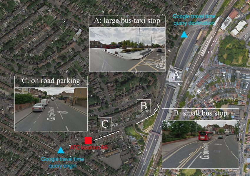
Data-Centric Engineering 19

Table 5. Speed MAE (km/h) by model form, road type and traffic volume level

 Volume-to-capacity ratio 100% Total

 obs. counts 383 245 375 366 23 1392
 % obs. counts 27.51 17.60 26.94 26.29 1.65 100
 Trunk Base 14.4 19.3 23.5 25.8 27.9 19.3
 Data 1 2.3 3.3 2.7 2.4 3.8 2.7
 Data 2 1.7 2.6 2.3 2.2 2.8 2.2

 obs. counts 1641 1082 1996 2746 216 7681
 % obs. counts 21.36 14.09 25.99 35.75 2.81 100.00
 Principal Base 13.3 17.2 18.9 21.1 21.5 18.7
 Data 1 1.9 2.2 2.9 2.8 3.4 2.6
 Data 2 1.8 2.0 2.5 2.6 2.5 2.4

 obs. counts 179 125 183 343 102 932
 % obs. counts 19.21 13.41 19.64 36.80 10.94 100.00
 B Base 9.0 6.6 4.3 3.5 3.8 4.8
 Data 1 1.8 2.3 4.6 6.7 8.6 3.6
 Data 2 1.8 2.1 2.2 2.1 2.2 2.1

 obs. counts 245 100 306 255 26 932
 % obs. counts 26.29 10.73 32.83 27.36 2.79 100.00
 C Base 20.7 21.9 21.6 21.1 19.4 20.7
 Data 1 1.8 2.1 2.3 3.4 4.9 2.4
 Data 2 1.7 1.9 1.6 1.7 1.5 1.6

 obs. counts 126 120 48 26 9 329
 % obs. counts 38.30 36.47 14.59 7.90 2.74 100.00
 Unclassified
 Base 24.7 25.5 26.0 27.0 30.6 26.0
 Data 1 2.1 1.3 2.3 4.7 3.7 2.3
 Data 2 2.0 1.2 1.3 2.3 3.4 2.0

7. Discussions on the limitations of the methodology
The empirical data gathered in this study vary significantly from the standard volume-delay curve. The
context-specific saturation delay and saturation speed functions and the standard BPR volume-delay
function show significant variations in the residuals. The large scatter observed in the volume-delay
relationship must be due to unknown external factors that have not been included in the candidate
models.

7.1. Example scenario & possible factors
Fig. 11 (a) presents the observed volume and delay scatter plot for ATC location 66 in both directions.
It is obvious that the southbound direction consistently experiences higher delay than the northbound
direction, even at same volumes of traffic. In an attempt to better understand and possibly explain this
distinct directional behaviour, satellite photography and street-level photography of the road is assessed.
Fig. 12 shows a satellite image of ATC location 66 obtained from Google Maps (Google Inc., 2020).
The red marker gives the location of the ATC counter itself, and the two blue markers illustrate the

20 Gerard Casey et al.

origin/destination location used in the Google Directions API request. From this satellite imagery and
street view imagery, possible explanatory factors can be identified:
1. The southbound lane features road parking;
2. The southbound lane features a large bus stop and taxi lay-by (for Leytonstone Station) and a
 smaller bus stop lay-by.
 The larger bus stop and taxi lay-by serving Leytonstone is a significant geometric feature that is
likely to have significant impact on the southbound traffic. The second smaller bus stop lay-by and
on-road parking may also have an impact, albeit to a smaller extent. Such factors may explain the
exhibited differences from the location-device-informed journey data and thus permit their inclusion in
an informal way.

7.2. Challenging scenarios
Inspections of the volume-delay scatter plots reveal a subset of roads that are not suitable to be described
with the BPR-style monotone function. For example, as previously explained in Section 5, 15 sites
are eventually removed from the analysis due to invalid data. Among the remaining 24 sites, many
have outliers even after the data cleaning process (e.g., Fig. 6). Fig. 11 (b) shows another “abnormal"
example, particularly with the northbound direction: the delay has a considerable variation when the
hourly volume is around 200 vehicles, far from its capacity of about 400 vehicles per hour. This is
probably resulted from the hyper-congested stage of the traffic, where the density has exceeded the
optimum value and flow decreases despite continuous increase in the delay. Such phenomena cannot
be correctly modelled by the monotone volume-delay function and should be dealt with using dynamic
models if the hyper-congested stage is crucial in the analysis (which is usually the case for short-term
predictions, such as evacuations). This is also reflected in the modeling guidance from the DfT, where
the preferred choice of modeling congested urban roads in traffic assignment is to explicitly represent
the junction delay and low cruise speed (DfT, 2020). The proposed data-driven models are useful in
certain scenarios, such as traffic assignment at the city-scale, where simplicity of the volume-delay
curves is crucial to ensure the computational tractability of the model. However, its limitation, namely
allowing unrealistic high traffic flow to be assigned to certain links, should be aware of. We plan to
compare the performance of the data-driven method with the more detailed models involving junctions
in our future work. The errors of using the monotonic volume-delay function in face of hyper-congested
real world observations are reflected in the MAE quantification as shown in Fig. 10. Apart from these
reasons, external factors could also affect the sensibility of the data, for example, a traffic collision or
flooding may result in a high level of delay in a short period of time.

7.3. Influencing factors
In Section 7.1 the existence of public transport infrastructure and on-road parking were identified as
being potentially explanations of the distinct southbound northbound behaviour on that road. A range
of other possible factors have been identified, which may help explain the unexplained variations:
1. Vehicle type
 In this study, all vehicles are considered to be the same, despite clear distinction in the interactions
 between two cars compared to an interaction of a car and a lorry (Vap et al., 2007). Further work
 is planned to assess the impact of the vehicle type. A wide variety of vehicles are observed on
 different road types, and such differences should be considered. The use of statistical vehicle mix
 sampled by road type (DfT, 2012b) was discounted for this study due to the small sample size of
 such statistics compared to the resolution of the data used here. The use of traffic cameras with
 number plate recognition and sufficient privileges to the Driver and Vehicle Licensing Agency

Data-Centric Engineering 21

Figure 11. Challenging scenarios: volume and delay observations at ATC site 66 (a) and 67 (b).

Figure 12. Satellite & Street View images of ATC 66 (Google Inc., 2020).

 (DVLA) database would enable the disaggregation of vehicle type at a similar spatial and
 temporal resolution to the Google Directions and DfT ATC data presented here.
2. Weather
 Weather events may impact the journey times by altering the functionality of the vehicle, the
 performance of the road and/or the performance of the driver. Ongoing research focuses on
 combining a large dataset of Google Directions journey times with data from the UK’s Met Office
 NIMROD precipitation dataset (The UK Met Office, 2003) to assess the relationship between
 these variables. At a microscopic level, it is known that an increase in precipitation increases
 journey times as a result of increased risk and the resulting decrease in vehicle speeds to
 compensate for this factor (Mashros et al., 2014).
3. Road incidents

22 Gerard Casey et al.

 Road works and road traffic collisions can lead to decreased or even zero capacity on a road link,
 resulting in increased saturation which impacts the journey time. Depending on the warning before
 such an event, the vehicle traffic may have the ability to adjust to this information, resulting in a
 greater distribution of traffic thus reducing the mediated travel times. Alternatively, an accident
 may occur without any warning to other road users committed to their route choice, resulting in
 longer journey time and perhaps gridlocks in the extreme cases. A method incorporating different
 accident and roadworks databases with Google Directions data is currently being investigated.
4. Road geometry, type & land use
 Different road layouts may increase the complexity of vehicle interactions. For example, the
 curvature of a corner and the road surface quality will impact the speed of a vehicle. The
 surrounding land use also has an influence on the vehicle speeds (for example, drivers take safety
 precautions near a school or leisure centre). The inclusion of such factors poses many challenges,
 including the size and complexity of the data plus the uncertainty and variability in how drivers
 react to the data. In Fig. 12, a series of geometric factors are displayed as an attempt to explain the
 different behaviours on the same road in different directions. The factors shown in Fig. 12 such as
 on-road parking and bus lay-bys could be quantitatively captured using computer vision and data
 sources such as Google Street View.

7.4. Generalisation and application
This study proposes an efficient data collection and processing pipeline for calibrating the macroscopic
volume-delay relationships for urban roads. The methodology considers the context-specific factors
that might affect such relationships but are hard to quantify using conventional approaches. Apart from
the challenges of using simple volume-delay curves in capturing the complex traffic behaviour, another
bottleneck for the proposed methodology is the availability of the data. This limitation comes in two
parts. First of all, the volume data could only be obtained for a small number of fixed locations, where
the ATCs are installed and can provide continuous traffic counts. The DfT also conducts manual traf-
fic surveys at a larger number of locations. However, these manual count data usually come at a lower
frequency (e.g., annual data) and may again miss the temporal network changes that have an impact
on traffic (e.g., roadworks). This bottleneck could be overcome in the near future by employing alter-
native data sources of traffic flow information, such as the information extracted from traffic cameras
using computer vision techniques (Drake, 2018). Secondly, the traffic speed data from Google (or other
mobility data providers) are not free, which may require the cost of acquiring data to be budgeted in for
large-scale studies. However, this method is expected to be cheaper and more scalable than collecting
the speed/delay data from conventional methods, such as the floating car data method.
 Nonetheless, the proposed methodology could still be beneficial in understanding the performance of
key network locations, such as bridges or major routes, when only point-based traffic measurements are
available. In addition, if more types of traffic sensors are installed in the future (e.g., radar or camera),
the proposed methodology could then be applied on a larger scale.

8. Conclusions
By combining two disparate data sources from the ATCs and Google’s traffic speed data, context-
specific volume-delay curves for a range of different locations and road types have been generated for
selected roads in Greater London. The derived volume-delay curves informed by real observational
data have shown significant improvements in capturing individual road characteristics compared to the
standard model. Apart from obtaining the site-specific knowledge, in a more practical use-case, the
derived functions could now be used in the traffic assignment stage of the traditional four-step model.
In some cases, the data presents clear evidence that unknown external factors, such as those listed in
Section 7.3, have a significant impact on the traffic behavior and warrant further investigation. In these