Revisiting the empirical fundamental relationship of traffic flow for highways using a causal econometric approach
←
→
Page content transcription
If your browser does not render page correctly, please read the page content below
Revisiting the empirical fundamental relationship of traffic flow
                                                  for highways using a causal econometric approach
                                                           Anupriya∗, Daniel J. Graham, Daniel Hörcher, Prateek Bansal
                                                        Transport Strategy Centre, Department of Civil and Environmental Engineering
                                                                                Imperial College London, UK

                                          Abstract
arXiv:2104.02399v1 [econ.EM] 6 Apr 2021

                                          The fundamental relationship of traffic flow is empirically estimated by fitting a regres-
                                          sion curve to a cloud of observations of traffic variables. Such estimates, however, may
                                          suffer from the confounding/endogeneity bias due to omitted variables such as driving
                                          behaviour and weather. To this end, this paper adopts a causal approach to obtain
                                          the unbiased estimate of the fundamental flow-density relationship using traffic detector
                                          data. In particular, we apply a Bayesian non-parametric spline-based regression approach
                                          with instrumental variables to adjust for the aforementioned confounding bias. The pro-
                                          posed approach is benchmarked against standard curve-fitting methods in estimating the
                                          flow-density relationship for three highway bottlenecks in the United States. Our em-
                                          pirical results suggest that the saturated (or hypercongested) regime of the estimated
                                          flow-density relationship using correlational curve fitting methods may be severely bi-
                                          ased, which in turn leads to biased estimates of important traffic control inputs such
                                          as capacity and capacity-drop. We emphasise that our causal approach is based on the
                                          physical laws of vehicle movement in a traffic stream as opposed to a demand-supply
                                          framework adopted in the economics literature. By doing so, we also aim to conciliate
                                          the engineering and economics approaches to this empirical problem. Our results, thus,
                                          have important implications both for traffic engineers and transport economists.

                                          Keywords: Fundamental relationship of traffic flow, endogeneity, causal econometrics,
                                          Bayesian machine learning, non-parametric statistics.

                                             ∗
                                                 Corresponding author. Email address: anupriya15@imperial.ac.uk

                                          Preprint submitted to Elsevier                                                          April 7, 2021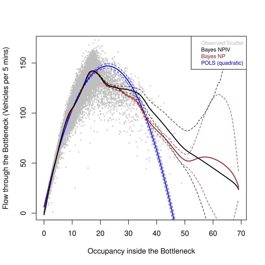
1. Introduction

   The standard engineering relationship between vehicular flow q, that is, the number
of vehicles passing a given point per unit time, and density k, that is, the number of
vehicles per unit distance in a highway section, as shown in quadrant (c) of Figure 1,
is commonly known as the fundamental relationship of traffic flow. This relationship is
defined based on the assumption that traffic conditions along the section are stationary,
which means that the three key traffic variables, q, k and average vehicular speed, v, are
the same at each and every point in the highway section (Daganzo, 1997; May, 1990).
Consequently, the relationship is basically estimated empirically by pooling observations
from different cross-sections along the highway across different time-periods and fitting
a regression curve to the point cloud. The estimation of such a curve follows from the
engineers’ interest in a general relationship to characterise the flow of traffic in a given
facility. The fundamental relationship can be equivalently expressed as speed-density or
flow-speed relationship, as shown in quadrants (a) and (b) of Figure 1, respectively.

 Figure 1: The fundamental diagram of traffic flow (adapted from Small and Verhoef, 2007)

   Engineers assert that the estimated relationship is a property of the road section, the
environment, and the population of travellers, because on an average, drivers show the
same behaviour (Daganzo, 1997). We argue that this estimated relationship, however,

                                             2
is at best only associational and possibly spurious due to several possible sources of
endogeneity/confounding biases. For instance, there are many external observed and
unobserved factors such as driver behaviour, heterogeneous vehicles, weather and demand,
that are correlated with the observed traffic variables (Mahnke and Kaupužs, 1999; Qu
et al., 2017), but are often omitted in the estimation of the fundamental relationship.
Fitting a pooled ordinary least square regression curve to the observed scatter plot of
traffic variables fails to adjust for the above-mentioned sources of confounding, which
may bias the estimated relationship (Wooldridge, 2010; Cameron and Trivedi, 2005).
The parametric limitations on functional form in regression further augments the bias in
the estimated relationship.
       To address these shortcomings of the traditional approach, in this paper, we estimate
the fundamental relationship between traffic flow and traffic density using a flexible causal
statistical framework. In particular, we adopt a Bayesian non-parametric instrumental
variables (NPIV) estimator (Wiesenfarth et al., 2014) that allows us to capture non-
linearities in the relationship with a non-parametric specification without presuming the
functional form and also adjust for any confounding bias via the use of instrumental
variables (IVs). We validate this approach using traffic detector data from three highway
bottlenecks located in California, USA1 . Thus, the main contribution of this research
lies in determining a novel causal (unbiased) relationship between traffic flow and traffic
density for a highway bottleneck.
       To the best of our knowledge, this study presents the first application of causal in-
ference in empirical estimation of the fundamental relationship from an engineering per-
spective that is based on the physics of movement of vehicles. We emphasise that some
economists have also adopted a causal framework for this problem in the past (see, for
instance, Couture et al., 2018). This framework is based on the interpretation of the
speed-flow fundamental relationship as the supply curve for travel in a road section un-
der stationary state traffic conditions (Small and Verhoef, 2007; Walters, 1961). We argue
that in developing a causal understanding of the fundamental relationship, the economic
representation of this model as a supply curve can lead to ambiguity. The economic

   1
    We choose highway bottlenecks over uniform highway sections to demonstrate that our approach not
only delivers an unbiased fundamental relationship for a highway section but also correctly estimates
capacity-drop, an important feature of the bottleneck section.

                                                 3
interpretation seeks stationary state traffic conditions, which seldom exist, particularly
under congested conditions.
    Based on this type of economic representation, a recent empirical study by Anderson
and Davis (2020, 2018) discards the existence of the hyper-congested2 part of the funda-
mental diagram (see Figure 1 to locate the hypercongested part). Note that for a highway
bottleneck, there are two components of the hypercongested regime of the fundamental
diagram: (i) the region representing capacity drop, that is, a sudden reduction in ca-
pacity of the bottleneck at the onset of upstream queuing, and, (ii) the region following
the capacity drop where the flow-density or flow-speed relationship is backward bending
as per the engineering literature. The absence of empirical evidence on the existence
of both components of hypercongestion (that is, reduction in traffic flow with increas-
ing traffic density or demand, Anderson and Davis (2020, 2018)) questions the relevance
of hypercongestion as a motivating factor for traffic controls measures and congestion
pricing strategies.3
    Through our proposed causal framework, we also aim to conciliate this recently diverg-
ing strand from the economics literature with the well-established engineering knowledge
on the existence of hypercongestion. Specifically, we contribute to the re-initiated debate
on the existence of hypercongestion in highways and deliver novel causal estimates of
capacity reduction in various highway bottlenecks. We emphasise that our estimates of
the capacity reduction are derived from the estimated fundamental relationship itself,
as opposed to the previous literature that uses different methodologies (e.g., change in
cumulative vehicle count) to quantify the phenomenon (see, for instance, Cassidy, 1998;
Oh and Yeo, 2012; Srivastava and Geroliminis, 2013). Thus, our proposed approach pro-
vides a one-stop solution to estimate an unbiased fundamental relationship as well as its
important features such as capacity and capacity-drop. As an important intermediate
research outcome of this study, we also undertake a critical evaluation of the assump-
tions underlying the economists’ treatment of the fundamental relationship as a supply
curve for travel, which may lead to inconclusive empirical evidence on the existence of

    2
      Whereas the engineering terminology for the backward bending region of the fundamental diagram
is ‘saturated flow’, economists call it ‘hypercongested’ (Small and Chu, 2003).
    3
      A few early studies in the engineering literature also report no capacity reductions (Hall and Hall,
1990; Persaud, 1987; Newman, 1961), however, their results have been found to be inconclusive owing to
the methods adopted in these studies (Cassidy and Bertini, 1999).

                                                    4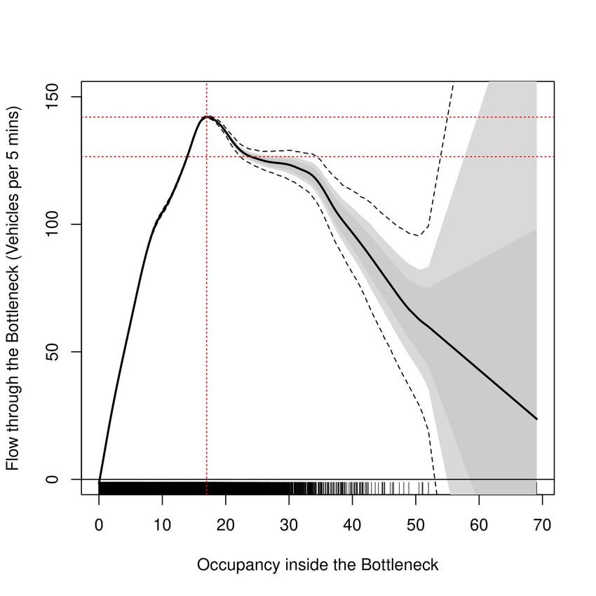
hypercongestion.
      The rest of this paper is organised as follows. Section 2 reviews the relevant engineer-
ing literature, critically examining the theoretical foundations underlying the empirical
estimation of the fundamental relationship between traffic variables. Additionally, we
also review the literature on capacity-drop in highway bottlenecks. Section 3 describes
the chosen study sites and the corresponding traffic detector data and variables. Section 4
details the model specification and the adopted methodology explaining how it addresses
endogeneity bias in the context of the fundamental relationship. Section 5 presents our
results and benchmarks them against those derived using a standard non-parametric es-
timator without instrumental variables. Furthermore, we compare our findings with the
relevant engineering and economics literature. Conclusions and implications are presented
in the final section.

2. Literature Review

      In this section, we discuss the theoretical foundations underlying the engineering
approach to estimate the fundamental relationship and the key shortcomings of this
approach. We also highlight how a causal econometric framework can be employed to
obtain a more robust characterisation of the fundamental relationship.

2.1. The empirical fundamental relationship

      As discussed in the introduction, the fundamental relationship is empirically esti-
mated using observations on traffic state variables that are averaged over time and/or
space. The averaging of observations requires strict assumptions like stationary traffic
and homogeneous vehicles. Note that empirical studies use occupancy, o, as a proxy for
traffic density because traffic density cannot be measured directly (Daganzo, 1997; May,
1990)4 . For a contextual discussion, Figure 2 shows a scattered plot of the measured
flow versus occupancy from a traffic loop detector (aggregated over 5 minutes) located
upstream of the Caldecott Tunnel in the SR24-W, California on several workdays.
      The conventional fundamental relationship is obtained by fitting a predefined curve
to the point cloud of aggregated data. While numerous functional forms have been
proposed (see Hall et al., 1993, for a review), most researchers agree that the flow-density

  4
      Occupancy is defined as the percentage of the sampling period for which vehicles occupy the detector

                                                     5
Figure 2: Conventional flow versus occupancy plot using detector data aggregated over 5 min-
utes.

relationship should either be triangular (Newell, 1993; Hall et al., 1986) or parabolic
(Greenshields et al., 1935; HCM, 2016). Proposed relations also include discontinuous
models whereby the functions describing unsaturated and saturated traffic regimes do
not come together to form a continuous curve (Payne, 1977; Ceder and May, 1976; Drake
and Schofer, 1966).
   As noted in previous studies, the data shows considerable scatter particularly in the
saturated regime, which has led some researchers to question the existence of reproducible
relationships in this regime (refer to May, 1990, for details). The challenges posed by this
scatter in obtaining an accurate fundamental relationship has stimulated the growth of
many interesting strands in the engineering literature: from understanding and account-
ing for the various sources of scatter (see, for instance, Cassidy, 1998) to introduction of
stochastic fundamental relationships (Wang et al., 2013) and fitting multi-regime models
(see, for instance, Kidando et al., 2020). The following subsections summarise the main
findings from our review.

                                             6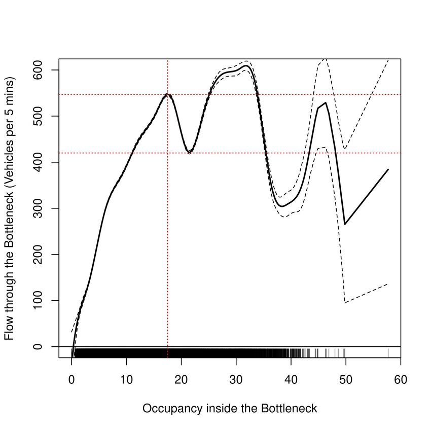
2.1.1. Characterising the sources of scatter
   Cassidy (1998) argued that data from brief periods of near-stationarity (that is, unsus-
tained periods of time over which the traffic stream is marked by nearly constant average
vehicle speeds) or non-stationary transitions do not always conform to near-stationary
relations because such data points arise due to random fluctuations in the traffic vari-
ables. Further, Cassidy (1998) showed that only data points from sustained periods of
near stationary traffic condition conform to well-defined reproducible bivariate relations
among traffic variables. Cassidy (1998) and Daganzo (1997) attribute such well-defined
relationships to the same average behaviour of drivers when confronted with the same
average traffic conditions.
   However, Coifman (2014a) found that even under strict stationary state traffic con-
ditions, aggregated measurements of flow, density (or occupancy) and speed may exhibit
large scatter in the queued regime arising from: (i) erroneous measurements of flow due
to non-integer number of vehicle headways in a given sampling period, (ii) averaging
over a small number of vehicles during low flow periods, (iii) measurement errors due
to detectors, (iv) the mixing of inhomogeneous vehicles (for instance, trucks and cars),
and, (v) the mixing of inhomogeneous driver behaviours. Consequently, Coifman (2014b)
relaxed the requirement to seek out strict stationary state conditions by measuring the
traffic state (flow and occupancy) for individual vehicles, followed by grouping of these
measurements by similar lengths and speeds. For each group, Coifman (2014b) derived
the flow-occupancy relationship by connecting points corresponding to the median flow
and median occupancy. Coifman (2014b) argues that the use of median instead of the
conventional use of mean controls for outliers arising from detector errors or uncommon
driver behaviour.
   We note that there are two main drawbacks of this approach. First, the method
is highly data-intensive and requires microscopic-level measurements on individual ve-
hicles. Second, although the method helps in estimating well-defined relationships for
homogeneous vehicle classes, a traffic stream seldom consists of homogeneous vehicles
only. This deficiency becomes a critical concern because the method does not clearly
suggest how to obtain an aggregate relationship for a mix of vehicles from class-specific
relationships, which is of general interest to devise traffic control measures and congestion
pricing strategies.

                                               7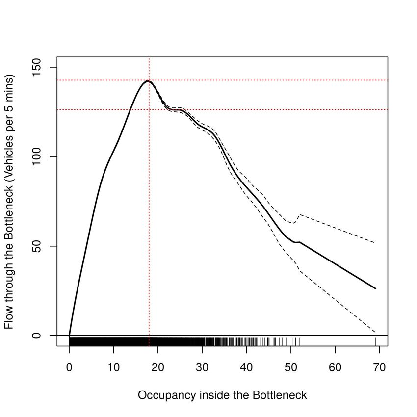
2.1.2. Stochastic fundamental relationships
   Consistent with Cassidy (1998), a series of other recent studies have attributed the
observed scatter to random characteristics of traffic behaviour (Qu et al., 2015; Chen
et al., 2015; Mahnke and Kaupužs, 1999; Qu et al., 2017; Muralidharan et al., 2011;
Jabari et al., 2014; Sopasakis, 2004). These studies suggest that the scatter arises due
to various external factors such as heterogeneous vehicles, driver behaviour, weather
conditions, and the random characteristics of demand. Previous empirical studies also
demonstrate how failure to adjust for the stochastic characteristic of traffic flow variables
in calibration of the fundamental relationship result into highly inaccurate models (Ni,
2015; Wang et al., 2011; Li et al., 2012).
   To account for these random characteristics, Wang et al. (2013) introduced a stochas-
tic fundamental relationship in place of traditional deterministic models, in which they
assume speed to be a random process of density and a random variable. Subsequently,
Hadiuzzaman et al. (2018) and Kidando, Moses and Sando (2019) have used Adaptive
Neuro Fuzzy Inference System and Markov Chain Monte Carlo (MCMC) simulations
respectively to capture the uncertainty in parameter estimates of the fundamental rela-
tionship arising due from the stochastic behaviour of traffic.
   We note that the baseline estimates of the flow-density or the speed-density curve
derived within the stochastic framework are based on a pooled ordinary least square
estimator. We argue that such estimates of the baseline curve may be confounded by the
extraneous factors discussed in the literature. We explain this confounding bias in detail
in Section 4.2.

2.1.3. Multi-regime models
   Traditional single-regime models (for instance, Greenberg, 1959; Pipes, 1966; Mun-
jal and Pipes, 1971) that assume a single, pre-defined shaped curve for the entire do-
main of the fundamental relationship have been found inaccurate because free-flow and
congestion-flow regimes have different flow characteristics (Ni, 2015; May, 1990; Hall
et al., 1993). As a consequence, multi-regime models have been introduced in the lit-
erature as a flexible alternative to increase the calibration accuracy of the fundamental
relationship. Multi-regime models fit different regimes of the fundamental relationship
with different pre-defined functional forms where regimes are separated by breakpoints or
thresholds (Edie, 1961; Drake, 1967; Sun and Zhou, 2005). Whereas two-regime models

                                              8
comprise of free-flow and congested-flow regimes, three-phase models additionally include
a transitional regime between free-flow to congestion, which is consistent with Kerner’s
three-phase traffic theory (Kerner, 2009).
   In most studies, modellers pre-define the locations of breakpoints based on the subjec-
tive judgement, which may significantly affect the accuracy of the estimated multi-regime
models (Wang et al., 2011; Sun and Zhou, 2005; Liu et al., 2019). Studies such as Kockel-
man (2001); Sun and Zhou (2005) and Kidando, Kitali, Lyimo, Sando, Moses, Kwigizile
and Chimba (2019) have thus focused on the estimation of these breakpoints based on a
user-driven choice of the number of regimes as input. Kidando et al. (2020) proposed a
fully data-driven Bayesian approach to estimate the breakpoints of multi-regime models,
but did not account for the potential confounding biases. Our flexible non-parametric ap-
proach does not require any user inputs regarding the shape of fundamental relationship,
automatically identifies such change-points in a data-driven manner and also accounts
for the possible confounding biases.

2.1.4. Research gaps and contributions
   Our review suggests that traffic engineers are interested in deriving a well-defined
reproducible relationships between traffic variables that can be attributed to the same
average behaviour of drivers under the same average traffic conditions. The develop-
ments in the engineering literature serve as an excellent starting point to understand the
sources of variation in traffic state measurements that leads to large scatter, particularly
in the congested regime of the fundamental diagram. While the previous studies on the
stochastic fundamental diagram rightly argue that the scatter arises due to various ex-
ternal factors, they do not appropriately adjust for the confounding bias that may occur
from these factors when estimating the aggregate (baseline) fundamental relationship.
We argue that these factors are likely to be highly correlated with the observed traffic
variables, thus, an ordinary least squares based estimation of the fundamental relation-
ship may be biased (see Section 4.2 for details). Moreover, most of the multi-regime
models require user inputs for calibration and ignoring the endogeneity bias remains the
concern.
   To fill these gaps in the literature, we introduce a methodological framework to es-
timate the fundamental relationship that can effectively control for confounding from
the external sources identified in the literature, alongside adjusting for other inherent

                                             9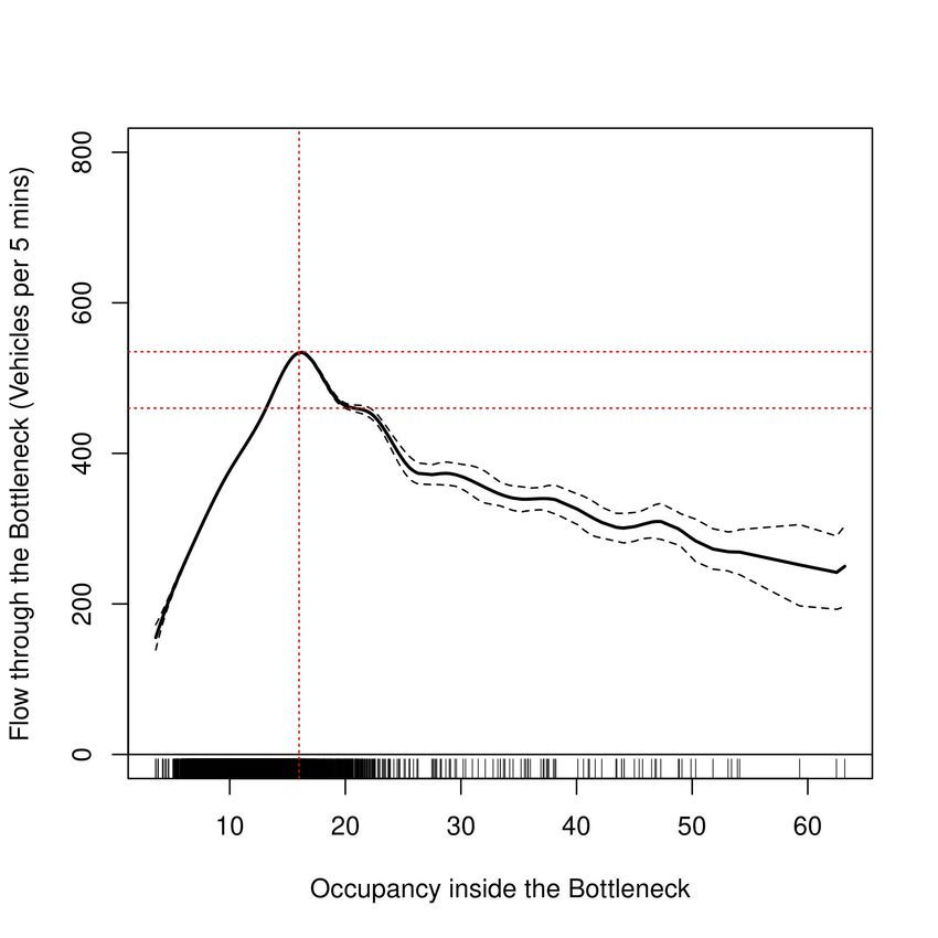
randomness in the data generating process, and produce a more general characterisation
of traffic flow for a highway section under an average mix of traffic. The adopted fully
flexible non-parametric specification for the fundamental relationship produces a multi-
regime fundamental relationship without any prior assumptions on either the shape of the
curve or the location of breakpoints. Moreover, as a by product of Bayesian estimation,
we also quantify the uncertainty in the estimated relationship with credible intervals.
Furthermore, important traffic control inputs for highway bottlenecks such as capacity
and capacity drop are also obtained as a by-product of the estimation. In the rest of this
section, we review the relevant literature on highway capacity and capacity drop to il-
lustrate the importance of quantifying these parameters from the estimated fundamental
diagram.

2.2. Highway Capacity and Capacity Drop

       Understanding the capacity of a highway section is critical in modelling of traffic flow
in highways (Srivastava and Geroliminis, 2013; Siebel et al., 2009; Laval and Daganzo,
2006)5 , particularly those with bottlenecks (such as lane drops and merges, among others).
This is because, the highway capacity at the bottleneck location may be insufficient for
traffic demand during peak hours and hence, traffic jams may occur. Capacity drop is
thus defined as the drop in discharge flow through a bottleneck, when it is activated with
an increase in demand. The activation of a bottleneck is marked by onset of queuing
upstream of the bottleneck Yuan et al. (2015); Oh and Yeo (2012); Chung et al. (2007);
Cassidy and Bertini (1999). The literature also acknowledges capacity drop as a two-
capacity phenomenon of active bottlenecks and relate it to the discontinuity observed
at capacity flows near saturation point in the flow-density or flow-speed fundamental
diagram. Several empirical observations of capacity drop ranging between 2 percent -
25 percent are found in the literature. Table 1 presents a summary of the capacity
drop reported in the literature for different highway sections with varying bottleneck
type. Based on the behavioural theory of traffic flow, Daganzo (2002) attributes the
capacity drop to a loss of motivation among drivers, that is, these drivers presumably

   5
     Note that there are many potential definitions of capacity in the literature (see Kondyli et al., 2017,
for a brief review). For instance, Cassidy and Rudjanakanoknad (2005) define capacity as the sustained
flow discharged from all highway exits that are unblocked by spillover queues from downstream while
the highway entrances are queued. Oh and Yeo (2012) define capacity as the maximum discharge flow
of vehicles that persist for 5 minutes in a free-flow state.

                                                    10
loose their willingness to drive at high speeds with small headways. In addition, Laval
and Daganzo (2006) and Leclercq et al. (2011) suggest that capacity drop occurs due to
voids in the traffic caused by lane changing. Past researchers also relate the differences in
capacity drop values with the number of lanes, severity of stop-and-go waves and speeds
in congestion Oh and Yeo (2012, 2015); Yuan et al. (2015).
Table 1: Summary of key literature on the existence capacity drop in highways.
Study Location Type Capacity Drop (%)
Banks (1990) I-8, San Diego on-ramp merge -0.42 to 1.11
Hall and Agyemang-Duah (1991) Queen Elizabeth Way, Toronto on-ramp merge -7.76 to 10.36
Banks (1991) Multiple Sites, San Diego merge/ lane drop/ weave 1.8 to 15.4
Persaud et al. (1998) Multiple Sites, Toronto on-ramp merge 10.6-15.3
Cassidy and Bertini (1999) Multiple Sites, Toronto on-ramp merge 4 to 10
Bertini and Malik (2004) US-169, Minneapolis on-ramp merge 2 to 5
Bertini and Leal (2005) M4, London merge 6.7 to 10.7
Cassidy and Rudjanakanoknad (2005) I-805, San Diego on-ramp merge 8.3 to 17.3
Chung et al. (2007) I-805, San Diego on-ramp merge 5 to 18
SR-24, California on-ramp merge, lane reduction 5.1 to 8.5
Gardiner Expressway, Toronto on-ramp merge, horizontal curve 3 to 12
Leclercq et al. (2011) M6, UK merge 25
Oh and Yeo (2012) Multiple Sites, California on-ramp merge 8 to 16.5
Srivastava and Geroliminis (2013) US-169, Minneapolis on-ramp merge 8 to 15
Jin et al. (2015) I-405, California merge 10.5
Anderson and Davis (2020) Multiple Sites, California lane reduction 0
*This table has been adapted from Oh and Yeo (2012).
The existence of capacity-drop in a highway section is well-recognised in the trans-
portation literature and has been a long-standing rationale for application of traffic con-
trols, such as, ramp metering (Cassidy and Rudjanakanoknad, 2005; Smaragdis et al.,
2004; Diakaki et al., 2000), and highway pricing and tolls (Hall, 2018b,a; Fosgerau and
Small, 2013; Newbery, 1989; Boardman and Lave, 1977; Walters, 1961) to regulate de-
mand. We note that the methods adopted in the literature to quantify capacity drop
differ substantially from each other. For instance, Banks (1990), Persaud et al. (1998),
Zhang and Levinson (2004) and many more study minute-to-minute variability in traffic
flows to infer decrease in high traffic flow levels. Studies like Bertini and Leal (2005)
and Cassidy and Rudjanakanoknad (2005) use cumulative vehicle counts to infer the re-
duction in flow at downstream detectors relative to upstream detectors. Srivastava and
Geroliminis (2013) study changes in bottleneck flows with respect to upstream density.
However, the capacity-drop phenomenon has recently been called into question in
the urban economics literature. Anderson and Davis (2020, 2018) study the changes
in capacity of a highway section with a bottleneck during periods of high demand for
three bottlenecks in California and conclude that there is no evidence of capacity drop,
hence, hypercongestion, in the absence of any infrastructure-related shocks (for instance,
11lane closures, traffic incidents and so on) and weather-based shocks. Consequently, they
question the relevance of hypercongestion in the design of traffic controls and congestion
pricing.
The capacity drop estimates in engineering studies are based on only a certain few
days of observations. Anderson and Davis (2020) instead use data from several hundred
days and adopt an event-study design to measure changes in highway capacity before and
after of queue formation averaged over all days. It is important to note that Anderson
and Davis (2020) select a speed threshold of 30 mph at the upstream detector closest to
the bottleneck to detect the onset of upstream queuing.
We argue that inferring the actual moment of queue formation using a speed threshold
for upstream detectors may lead to ambiguity. We instead reevaluate the capacity drop
phenomenon by deriving estimates of capacity drop from the causal estimate of the flow-
occupancy relationship at the bottleneck location. However, as rightly suggested by
Anderson and Davis (2020), we use several months of observations to separate capacity
drop from minute-to-minute fluctuations in traffic flow.
3. Data and Relevant Variables
We make use of traffic data from three standard highway sections with distinct geome-
try, each having a single and clearly identified active bottleneck located at its downstream
end. At all of the chosen sites, slowing down of traffic and queuing is observed at the
bottleneck location. The associated high-quality data is collected via a series of loop
detectors installed at various locations along the highway, which measure traffic flow and
occupancy averaged over every 5-minute duration. The data is maintained by the Cal-
ifornia Department of Transportation (Caltrans) and made publicly available through
their Performance Measurement System (PeMS) website6 .
3.1. Study Sites
3.1.1. Site 1
The first bottleneck that we study is located in the westbound direction of the Califor-
nia State Route 24 (SR-24) at the Caldecott Tunnel in Oakland, California. The SR-24
connects suburban Contra Costa County in the East Bay region of the San Francisco
6
Performance Measurement System (PeMS) website: http://pems.dot.ca.gov/
12Bay Area with the cities of Oakland and San Francisco in the west. During the pe-
riod 2005-2010, the Caldecott tunnel was operated with two reversible lanes carrying the
westbound traffic in the morning and the eastbound traffic in the afternoon and evening.
Thus, for afternoon and evening hours of the above period, the location features an ac-
tive bottleneck in the westbound direction with the number of lanes decreasing from four
to two. As the traffic approaches the tunnel, traffic delays being quite common at this
location (previously studied by Chin and May, 1991; Chung et al., 2007; Anderson and
Davis, 2020, among others). We use observations on the westbound traffic in the time
period 12:00-24:00 hours on weekdays in the months of June-August during 2005-2010.
This highway section is well-isolated, that is, located well away from any major down-
stream intersection. Consequently, we assume that this section allows us to study traffic
dynamics arising solely from the presence of the bottleneck, without being affected by
any downstream influences.
3.1.2. Site 2
Our second study site is located in the eastbound direction of the California State
Route 91 (SR-91). SR-91 connects several regions of the Greater Los Angeles urban area
in the west with the Orange and Riverside Counties in the east. At the location where two-
lane traffic from the Central Avenue- Magnolia Centre in the Riverside Country merges
with its three-lane eastbound traffic, it features an active merge bottleneck (previously
studied by Oh and Yeo, 2012). This bottleneck appears as one of the top 100 bottlenecks
in California enlisted on the PEMS website with queuing and delays being quite common
at this location during morning and evening hours. We use observations on the eastbound
traffic in the time period 06:00-12:00 hours on weekdays in the months of June-August
during 2009-2014. This highway section is also well-isolated, thus, the traffic dynamics
arising within the section arise solely from the presence of the bottleneck.
3.1.3. Site 3
The third bottleneck that we study is located in the eastbound direction of Califor-
nia State Route 12 (SR-12). SR-12 connects the Sonoma, Napa, and Solano Counties,
following which it merges with Interstate 80 (I-80) which continues north towards Sacra-
mento. At a location just west of I-80, the number of lanes in the highway drops from two
lanes to one. This site has been previously studied by Anderson and Davis (2020) who
13suggest that the lane-drop results in the formation of an active bottleneck with queues
that are often very long. We use observations on the eastbound traffic in the time period
12:00-24:00 hours on weekdays in the months of May-August during 2018-2019.
Further downstream of the lane drop, the SR-12 merges with I-80. However, Anderson
and Davis (2020) note that the dynamics within this section are not affected by this merge.
We adopt this section for further analysis as it offers an interesting avenue to verify the
effect of downstream influences on the estimated fundamental relationship within the
bottleneck.
3.2. Relevant Variables
A schematic representation of the three bottlenecks, along with the location of detec-
tors that we use to obtain the relevant data, is shown in Figure 3.
For the first site, we observe a set of two detectors downstream of the lane-drop (that
is, within the bottleneck) and four detectors upstream to it. For the second site, we
observe a set of three detectors downstream of the merge (that is, within the bottleneck)
and three detectors upstream to it. For the third site, we observe one detector downstream
of the lane-drop (that is, within the bottleneck) and two detectors upstream to it.
It is also worth emphasising that for all the three bottlenecks, there are no reasonable
alternative routes to the highway section for the analysed traffic. We can thus assume
that, on an average, driver population using the section during the study period does
not differ substantially on weekdays. Table 2 summarises the relevant variables from the
three sites that are used in this study.
14(a) A lane-drop bottleneck in the westbound SR-24 in Oakland, California.
(b) A merge bottleneck in the eastbound SR-91 in Riverside, California.
(c) A lane-drop bottleneck in the eastbound SR-12 in Solano,
California.
Figure 3: Schematic representation of the study sites.
15Table 2: Summary statistics for variables used in this analysis.
(a) Site 1: SR-24 westbound.
Variable Detectors Obs. Min Max Mean Std.Dev
Traffic Flow (veh/5mins) Gateway Blvd 54432 0.00 595.00 249.58 77.57
Occupancy Gateway Blvd 54432 0.00 73.60 18.82 18.16
Traffic Flow (veh/5mins) Fish Ranch Rd 54432 0.00 760.00 383.95 149.57
Occupancy Fish Ranch Rd 54432 0.00 57.70 12.29 7.19
(b) Site 2: SR-91 eastbound.
Variable Detectors Obs. Min Max Mean Std.Dev
Traffic Flow (veh/5mins) Central EB ON 27936 102.00 593.00 372.21 53.03
Occupancy Central EB ON 27936 3.60 57.90 11.20 5.08
Traffic Flow (veh/5mins) W/O IVY 27936 152.00 628.00 393.55 69.77
Occupancy W/O IVY 27936 3.60 63.20 10.89 3.09
Traffic Flow (veh/5mins) Central On-ramp 27936 0.00 131.00 35.99 33.33
(c) Site 1: SR-12 eastbound.
Variable Detectors Obs. Min Max Mean Std.Dev
Traffic Flow (veh/5mins) W/O Red Top Rd 24908 0.00 210.00 102.13 43.08
Occupancy W/O Red Top Rd 24908 0.00 74.90 18.64 19.44
Traffic Flow (veh/5mins) Red Top Rd 24908 0.00 173.00 99.68 43.71
Occupancy Red Top Rd 24908 0.00 69.10 11.41 6.84
4. Methodology
This section is divided into four subsections. In the first subsection, we discuss the
model specification. In the second subsection, we explain potential endogeneity bias in
estimation of the fundamental relationship. In the penultimate subsection, we briefly
review NPIV methods in the literature and describe the Bayesian NPIV method in the
context of this study. In the concluding section, we benchmark the performance of the
Bayes NPIV estimator against state-of-the-art estimators in a Monte Carlo study and
illustrate its superiority in adjusting for endogeneity bias and recovering complex func-
tional forms.
4.1. Model Specification
We estimate a causal relationship between occupancy inside the bottleneck, obit , in
the five-minutes interval i, i = 1, .., N , on a particular day t, t = 1, ..., T , and the flow
through the bottleneck, qitb . We consider qitb to be a function of obit , conditional on the
properties of the infrastructure, the environmental conditions and the average behaviour
16of drivers and vehicles.
qitb = S b (obit ) + δitb + ξitb (1)
where δitb includes the unobserved (to researchers) traffic-specific behavioural component
common to all drivers, traffic-specific vehicular attribute common to all vehicles, weather-
specific component affecting the entire traffic stream, and demand-related characteristic.
ξitb represents an idiosyncratic error term representing all random shocks to the dependent
variable. Since the exact structural form of how obit enters into equation is unknown, we
adopt a non-parametric specification of S b (.). δitb is expected to be correlated with obit .
We explain the implications of this correlation on the estimated relationship in the next
subsection (Section 4.2).
As a by-product of this estimation, we quantify the activation of the bottleneck as
follows. Consistent with the engineering literature, we consider that the flow through the
bottleneck drops following the activation of the bottleneck. Thus, we infer the critical
value of obc at which we observe a significant backward bending in q b from the estimated
relationship S b (.). We also note that when the occupancy inside the bottleneck remains
at and above obc , the bottleneck remains activated.
Through the estimated relationship, we quantify the capacity of the bottleneck qcb ,
that, is flow through the bottleneck corresponding to obc and examine the existence of
capacity drop or two-capacity phenomenon following the activation of the bottleneck.
4.2. Bias due to Endogeneity
Building a credible causal relationship between traffic variables requires the under-
standing of potential endogeneity biases. There are two major concerns in relation to
endogeneity: omitted variable bias and reverse causality (simultaneity). Omitted covari-
ates that are correlated with both the dependent variable and the included covariates in
a regression may result in inconsistent estimates of model parameters. For instance, in
equation 1, omission of covariates representing driving behaviour of users due to unavail-
ability of a comprehensive aggregate level measure may lead to confounding bias in the
estimated relationship. This bias occurs because driving behaviour may be correlated
with both occupancy and flow. Reverse causality is a consequence of the existence of a
two-way causal relationship or a cause-effect relationship, contrary to the one assumed in
17the model. For instance, in equation 1, we assume the flow through the bottleneck, qitb to
be a function of the occupancy inside the bottleneck, obit . However, there may be reverse
causality where qitb affects obit in certain traffic situations. The presence of reverse causality
may also lead to inconsistent estimates. We further mathematically demonstrate the two
sources of confounding and resulting biases in Appendix A.
4.3. Bayesian Nonparametric Instrumental Variable Approach
To address both endogeneity biases, we adopt regression estimators with instrumen-
tal variables (IV). IV-based estimators such as two-stage least squares (2SLS) are widely
adopted in applied econometrics to estimate parametric models that contain endogenous
explanatory variables (see, for example Wooldridge, 2010). However, finite-dimensional
parametric models for the fundamental relationship of traffic flow such as a linear speed-
density or a quadratic flow-speed model, are based on assumptions that are rarely jus-
tified by engineering or economic theories. The resulting model mis-specification may
lead to erroneous estimates of attributes characterising the fundamental relationship (for
instance, capacity or capacity drop). On the other hand, non-parametric methods have
the potential to capture the salient features in a data-driven manner without making a
priori assumptions on the functional form of the relationship (Horowitz, 2011). There-
fore, a fairly growing strand in the econometrics literature proposes different approaches
for non-parametric instrumental variables (NPIV) regression, but such methods have
not been considered in the estimation of fundamental diagram. Extensive reviews can be
found in Newey and Powell (2003) and Horowitz (2011). The NPIV approaches are either
based on regularisation or control function. In this study, we adopt a control-function
based Bayesian NPIV estimator (Wiesenfarth et al., 2014). In what follows, we start
with the general model set-up. Subsequently, we discuss the advantages of the adopted
control-function-based Bayesian approach. Additionally, in Appendix B, we summarise
the challenges associated with regularisation based approaches that are more commonly
adopted in the empirical economics literature.
We first rewrite equation 1 in a traditional two-stage IV-based regression set up:
q = S(o) + 2 , o = h(z) + 1 (2)
with response q, endogenous covariate o, IV z for o and idiosyncratic error terms 1 and 2
18for the first and second stage regressions, respectively. For the notational simplicity, we
drop time-day subscripts and superscripts. Note that δ in equation 1 are encapsulated
in 2 . Endogeneity bias arises as E(2 |o) 6= 0. We assume the following identification
restrictions:
E(1 |z) = 0 and E(2 |1 , z) = E(2 |1 ), (3)
which yields
E(q|o, z) = S(o) + E(2 |1 , z) = S(o) + E(2 |1 )
(4)
= S(o) + ν(1 ),
where ν(1 ) is a function of the unobserved error term 1 . This function is known as the
control function.
4.3.1. Control function-based approaches
Several control function-based approaches to estimation of equation 2 in the literature,
ˆ from the first stage are
adopt a two-stage approach where residuals ˆ1 , that is, o − h(z)
used as additional covariate in the second stage (for details, see Newey and Powell, 2003).
However, as pointed out by Wiesenfarth et al. (2014), such two-stage approaches have
certain limitations. First, the uncertainty introduced by estimating the parameters in
the first stage remains unincorporated in the second stage. Second, a precise estimate
of ν(1 ) to achieve full control for endogeneity is difficult to obtain because the focus is
on minimising the error in predicting o in the first stage. Third, a robustness control
is required to account for outliers and extreme observations in 1 that may affect the
endogeneity correction.
Bayesian control-function-based approaches can address these shortcomings of fre-
quentist counterparts and regularisation-based approaches by estimating equation 2 as
a simultaneous system of equations, allowing for automatic smoothing parameter selec-
tion for a precise estimation of the control function and for construction of simultaneous
credible bands 7 .
7
Credible bands are the Bayesian analogue to confidence bands in the frequentist set up that represent
the uncertainty of an estimated curve.
19However, early Bayesian control-function-based approaches consider a bivariate Gaus-
sian distribution of errors (1 , 2 ) ∼ N (0, Σ) (for instance, see Chib et al., 2009). This
σ12
assumption leads to linearity of the conditional expectation as, E(1 |2 ) = σ12
, where
σ12 = cov(1 , 2 ) and σ12 = var(1 ), restricting the control function to be linear in 1
(Wiesenfarth et al., 2014; Conley et al., 2008). Since outliers can be a common source of
non-linearity in error terms, they can aggravate the robustness issues of such linear spec-
ifications. To overcome these limitations, Conley et al. (2008) proposed the application
of a Dirichlet process mixture (DPM) prior to obtain a flexible error distribution, but
still relied on linear covariate effects. The method proposed by Wiesenfarth et al. (2014)
and adopted in this study, extends the approach by Conley et al. (2008) and allows for
fully-flexible covariate effects.
4.3.2. Adopted Bayesian NPIV approach (Wiesenfarth et al., 2014)
The Wiesenfarth et al. (2014)’s Bayesian NPIV approach thus allows us to correct for
endogeneity bias in regression models where the covariate effects and error distributions
are learned in a data-driven manner, obviating the need of a priori assumptions on the
functional form.
To satisfy the identification restrictions presented in equation 3, we need an instru-
mental variable (IV) z. The IV should be (i) exogenous, that is, uncorrelated with 2 ;
(ii) relevant, that is, correlated with the endogenous covariate o, conditional on other
covariates in the model. Due to the absence of suitable external instruments, we use an
aggregate lagged level of the endogenous covariate (occupancy) as an instrument. Specif-
ically, for occupancy observed in the five-minutes interval i on day t, we consider the
average of observations on the covariate from the interval i − 15 to i + 15 from the previ-
ous workday t − 1 as its instrument. We argue that the occupancy obit in the five-minutes
interval i on day t is correlated with the occupancy ob[i−15,i+15],t−1 in the thirty-minutes in-
terval surrounding i on the previous day t − 1. This correlation follows from the influence
of time-of-the-day on demand and from the fact that there are no reasonable alternative
routes to the highway sections being studied, so the population of drivers using the section
in the duration i over different workdays may not differ substantially. Moreover, as the
highway infrastructure remains unaltered during the study period, we expect the average
driving behaviour and thus traffic density to not differ substantially over different days
as the drivers are already conversant with the route. However, these lagged occupancy
20values ob[i−15,i+15],t−1 are exogenous because they do not directly determine the response
variable qitb in equation 1 and would never feature in the model for that response. To jus-
tify the relevance of the considered instrument, we present the estimated h(.) in equation
2 and complimentary results from Stock and Yogo (2005) weak instrument F-tests in the
Results and Discussion Section (Section 5.2.2).
Conditional on the availability of an instrument, the Bayesian NPIV estimator can
correct for the confounding bias. To account for nonlinear effects of continuous covari-
ates, both S(.) and h(.) (refer equation 2) are specified in terms of additive predictors
comprising penalised splines. Each of the functions S() and h(.) is approximated by a
linear combination of suitable B-spline basis functions. The penalised spline approach
uses a large enough number of equidistant knots in combination with a penalty to avoid
over-fitting. Moreover, the joint distribution of 1 and 2 is specified using nonparametric
Gaussian DPM, which ensures robustness of the model relative to extreme observations.
Efficient Markov chain Monte Carlo (MCMC) simulation technique is employed for a
fully Bayesian inference. The resulting posterior samples allow us to construct simulta-
neous credible bands for the non-parametric effects (i.e., S(.) and h(.)). Thereby, the
possibility of non-normal error distribution is considered and the complete variability is
represented by Bayesian NPIV. We now succinctly discuss specifications of the kernel
error distribution and computation of credible bands in Bayesian NPIV.
To allow for a flexible distribution of error terms, the model considers a Gaussian
DPM with infinite mixture components, c, in the following hierarchy:
∞
X
(1i , 2i ) ∼ πc N(µc , Σc )
c=1
(µc , Σc ) ∼ G0 = N(µ|µ0 , τΣ−1 Σ) IW(Σ|sΣ , SΣ )
c−1
! c−1
X Y (5)
π c = υc 1 − (1 − πj ) = υc (1 − υj ),
j=1 j=1
c = 1, 2, ...
υc ∼ Be(1, ζ).
where µc , Σc and πc denote the component-specific means, variances and mixing pro-
portions. The mixture components are assumed to be independent and identically dis-
tributed with the base distribution G0 of the Dirichlet process (DP), where G0 is given
21by a normal-inverse-Wishart distribution. The mixture weights are generated in a stick-
breaking manner based on a Beta distribution with concentration parameter ζ > 0 of
the DP. The concentration parameter ζ determines the strength of belief in the base
distribution G0 .
4.3.3. Estimation Practicalities
We exclude Gibbs sampler of Bayesian NPIV for brevity, but mainly focus on im-
plementation details and posterior analysis. Interested readers can refer to Wiesenfarth
et al. (2014) for derivation of conditional posterior updates.
We adapt BayesIV and DPpackage in R to estimate Bayesian NPIV. We consider
50,000 posterior draws in the estimation, exclude the first 15,000 burn-in draws and keep
every 10th draw from the remaining draws for the posterior analysis. The point-wise
posterior mean is computed by taking the average of 3,500 posterior draws. Bayesian
simultaneous credible bands are obtained using quantiles of the posterior draws. A si-
multaneous credible band is defined as the region Iδ such that PS|data (S ∈ Iδ ) = 1 − δ,
that is, the posterior probability that the entire true function S(.) is inside the region
given the data equals to 1 − δ. The Bayesian simultaneous credible bands are constructed
using the point-wise credible intervals derived from the δ/2 and 1 − δ/2 quantiles of the
posterior samples of S(.) from the MCMC output such that (1 − δ)100% of the sampled
curves are contained in the credible band. Similar process is used to obtain the credible
intervals of h(.).
4.4. Monte Carlo Simulations
We succinctly demonstrate the ability of the adopted Bayesian NPIV approach in
addressing challenges of functional form mis-specification and endogeneity in an instance
of a Monte Carlo study. We benchmark the Bayesian NPIV method against state-of-
the-art estimators to illustrate how this method is robust to both issues. In the data
generating process (DGP), we consider a concave regression function, that is, a fourth
degree polynomial specification but our conclusions are applicable for a more complex
specification.
22We use a sample of 10000 observations, with the following DGP:
y = −40x4 + 40x3 + 30w4 + 2
(6)
x = 3.5z + 2.1w + 1
where z and w are independent and uniformly distributed on [0,1]. 1 and 2 are inde-
pendent and identically distributed draws from the N [0,0.5] distribution. The variables
y represents the primary response variable, x denotes the endogenous covariate and z
represents the instrumental variable. The variable w captures the unobserved effects in
the model, that is, we assume that the analyst is ignorant of its presence in the true data
generating process for the dependent variable. We thus introduce one possible source of
confounding into the model: a positive correlation between the unobserved effect w and
the endogenous covariate x.
We note that the model set-up is similar in structure to equation 2, that is:
y = s(x) + 2
(7)
x = h(z) + 1
We apply four different estimators to estimate the curve s(x):
1. A two-stage least square (2SLS) estimator with a quadratic specification for s(x).8
2. A two-stage least square (2SLS) estimator with the true specification for s(x).
3. A Bayesian non-parametric estimator without instrumental variables (Bayes NP).
4. A Bayesian non-parametric estimator with instrumental variables (Bayes NPIV).
In the latter two approaches, we take 40000 Posterior draws to ensure stationarity
of Markov chains. For the posterior analysis, the initial 10000 draws were discarded
for burn-in and every 40th draw of the subsequent 30,000 draws was used for posterior
inference. Figure 4 overlays the estimated s(x) from the four approaches and true s(x).
We note that a 2SLS estimator with the true specification for s(x) is able adjust for the
endogeneity bias and could produce an unbiased estimate of s(x). However, in practice,
it is infeasible for the analyst to know the correct functional form specification a priori. A
functional form mis-specification can produce a highly biased estimate of s(x), as shown
8
Instead of a traditionally-used linear specification, we choose quadratic specification in 2SLS because
the scatter plot of the data would intuitively suggest the analyst to use such functional form of s(x).
23Figure 4: Comparison of different estimators in the Monte Carlo study.
by the estimated s(x) using the 2SLS estimator with a quadratic specification for s(x).
This exercise thus illustrates the importance of adopting a fully flexible non-parametric
specification for s(x) in a relationship.
However, in the presence of endogeneity, a traditional non-parametric estimator may
fail to produce an unbiased estimate of s(x). From Figure 4, we note that the curve
produced by the Bayes NP is highly biased. Adopting an estimator such as the Bayes
NPIV allows to adjusts for the endogeneity bias and produce an unbiased estimate of the
curve s(x).
In summary, this Monte Carlo exercise shows that the Bayes NPIV estimator, the one
adopted in this study, outperforms other parametric and non-parametric approaches as
it is allows for a fully flexible functional form specification and controls for any potential
24confounding bias.
5. Results and Discussion
This section is divided into two subsections. In the first subsection, we compare
results of the adopted Bayesian NPIV estimator with those of a Bayesian NP estimator
and a pooled ordinary least squares (POLS) estimator with a quadratic specification.
The Bayesian NP estimator is a counterpart of the Bayesian NPIV, which does not
address confounding bias (that is, z = x; 1 = 0; h(.) : identity function in Equation 2).
Furthermore, we discuss the estimates of the capacity and capacity-drop in detail and
compare these values with those reported in the literature. In the next subsection, we
present the estimated kernel error distributions to illustrate the importance of the non-
parametric DPM specification. The relevance of our instruments is also demonstrated in
this subsection.
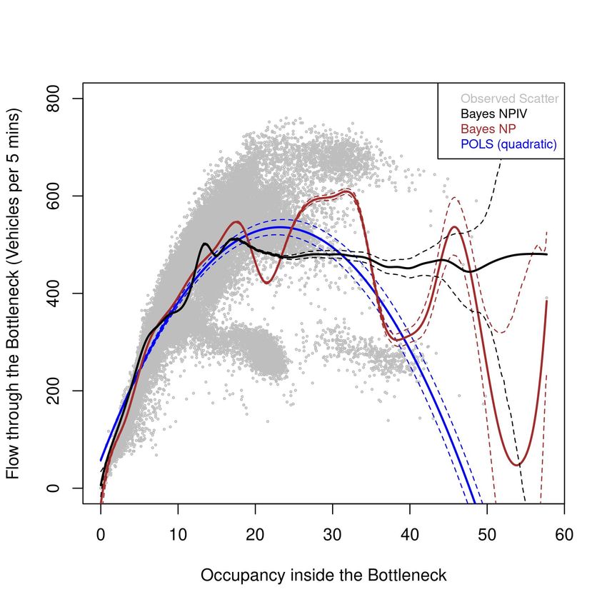
5.1. Comparison of Bayesian NPIV and non-IV-based estimators
We present the estimates of S(.) (see equation 2, second-stage) using Bayesian NPIV,
Bayesian NP, and POLS in Figures 5, 6 and 7 for the three highway sections. POLS
results are mainly presented to illustrate how commonly-used parametric non-IV-based
specifications can result biased results, but most discussion would revolve around com-
paring results of Bayesian NPIV and its non-IV counter part (that is, Bayesian NP).
From each of these figures, we do not observe any notable differences between the
Bayesian NPIV and Bayesian NP estimate of the free-flow regime of the flow-occupancy
curve. In this regime, the Bayesian NPIV estimate of S(.) is as efficient as its Bayesian NP
counterpart, as evidenced by tight credible bands in the domain of occupancy where we
have sufficient number of observations (note that the density of the tick marks on the X-
axis represents the number of observations). However, we observe substantial differences
near the saturation (capacity) point and in the congested (or hypercongested as per the
economics literature) regime of the estimate curve (see Figures 5(c), 6(c) and 7(c)). We
further discuss these differences in detail in next sub-sections.
25(a) Non-parametric non-IV estimator. (b) Non-parametric IV-based estimator.
(c) Comparison of different estimators.
Figure 5: Estimated flow-occupancy curves for Westbound SR-24.
26(a) Non-parametric non-IV estimator. (b) Non-parametric IV-based estimator.
(c) Comparison of different estimators.
Figure 6: Estimated flow-occupancy curves for Eastbound SR-91.
27(a) Non-parametric non-IV estimator. (b) Non-parametric IV-based estimator.
(c) Comparison of different estimators.
Figure 7: Estimated flow-occupancy curves for Eastbound SR-12.
28Table 3: Summary of Results.
(a) Comparison of estimators.
Estimated Capacity (veh/hr) Estimated Capacity-drop (percent)
Highway Section Bayes NP Bayes NPIV Bayes NP Bayes NPIV
Westbound SR-24 6561.12 6141.00 27.42 7.80
(12.00) (15.24)
Eastbound SR-91 6407.52 6997.44 14.02 n.s.
(5.16) (30.96)
Eastbound SR-12 1709.40 1708.20 11.54 10.92
(1.44) (1.68)
*n.s. stands for not statistically significant.
**Figures in bracket indicate the associated standard errors.
(b) Estimated capacity and comparison with the literature.
Highway Section Estimated Capacity Capacity reported in the Engineering literature
Westbound SR-24 6141 veh/hr 4100 veh/hr (Chung et al., 2007)
Eastbound SR-91 6997 veh/hr 7200 veh/hr (Oh and Yeo, 2012)
Eastbound SR-12 1708 veh/hr NA
*NA stands for not available.
**Figures in bracket indicate the associated standard errors.
(c) Estimated capacity-drop and comparison with the literature.
Estimated Average Capacity-drop as reported in the
Highway Section Capacity-drop Engineering literature Economics literature
Westbound SR-24 7.80 percent 5.10 to 8.40 percent n.s.
Eastbound SR-91 n.s. 13.50 percent NA
Eastbound SR-12 10.92 percent NA n.s.
*n.s. stands for not statistically significant; NA stands for not available. ´
(d) Activation of the bottleneck.
Occupancy corresponding to capacity
Highway Section non-IV-based IV-based
Westbound SR-24 17.56 17.27
Eastbound SR-91 16.13 17.50
Eastbound SR-12 17.71 17.08
295.1.1. Estimated capacity
Table 3a summarises the estimated capacity for each highway section. For Westbound
SR-24 that features a lane-drop bottleneck with number of lanes reducing from four
to two, the capacity estimated via the Bayesian NP estimator, that is, 546.76 (1.00)
vehicles per five-minutes or 6561.12 (12.00) vehicles per hour, is significantly more that
the Bayesian NPIV-based estimate, that is, 511.75 (1.27) vehicles per five-minutes or
6141.00 (15.24) vehicles per hour (see Figure 5). The capacity reported in the engineering
literature is 4100 vehicles per hour (refer to Table 3b), which is much lower than both of
these estimates.
For Eastbound SR-91 that features a merge bottleneck, Bayesian NPIV-based esti-
mate of capacity is 583.12 (2.58) vehicles per five-minutes or 6997.44 (30.96) vehicles
per hour, which is significantly higher that the Bayesian NP-based estimate of 533.96
(0.43) vehicles per five-minutes or 6407.52 (5.16) vehicles per hour (see Figure 6) but is
consistent with the value reported in the engineering literature (7200 vehicles per hour,
see Table 3b).
For Eastbound SR-12 that features a lane-drop bottleneck with number of lanes re-
ducing from two to one, the capacity estimated via the Bayesian NP-based estimator,
that is, 142.45 (0.12) vehicles per five-minutes or 1709.40 (1.44) vehicles per hour, is
similar to the Bayesian NPIV-based estimate of 142.35 (0.14) vehicles per five-minutes
or 1708.20 (1.68) vehicles per hour (see Figure 7). We do not note any previous estimate
of capacity of this section from the literature.
The above comparison does not point towards a clear direction of bias in the Bayesian
NP-based estimate of capacity with respect to the Bayesian NPIV-based estimate, rather
it varies on a case-by-case basis depending upon the data generating process. Failing to
address endogeneity bias leads to an over-estimation, an under-estimation and no differ-
ence in the estimated capacity for the first, second and third sections, respectively. We
also find the Bayesian NPIV-based estimates to be much closer to the previous estimates
from the engineering literature, particularly for Eastbound SR-91. However, a substantial
difference between our Bayesian NPIV estimate and the one reported in the engineering
literature for Westbound SR-24 can be attributed to the bias in previous estimates due
to minute-to-minute fluctuations in flow which might have caused due to the use of only
a few days of observations (Anderson and Davis, 2020). We emphasise that our causal
30You can also read