Back calculation of the 2017 Piz Cengalo-Bondo landslide cascade with r.avaflow: what we can do and what we can learn
←
→
Page content transcription
If your browser does not render page correctly, please read the page content below
Nat. Hazards Earth Syst. Sci., 20, 505–520, 2020
https://doi.org/10.5194/nhess-20-505-2020
© Author(s) 2020. This work is distributed under
the Creative Commons Attribution 4.0 License.

Back calculation of the 2017 Piz Cengalo–Bondo landslide cascade
with r.avaflow: what we can do and what we can learn
Martin Mergili1,2 , Michel Jaboyedoff3 , José Pullarello3 , and Shiva P. Pudasaini4
1 Institute of Applied Geology, University of Natural Resources and Life Sciences (BOKU),
Peter-Jordan-Straße 82, 1190 Vienna, Austria
2 Geomorphological Systems and Risk Research, Department of Geography and Regional Research,

University of Vienna, Universitätsstraße 7, 1010 Vienna, Austria
3 Institute of Earth Sciences, University of Lausanne, Quartier UNIL-Mouline, Bâtiment Géopolis,

1015 Lausanne, Switzerland
4 Institute of Geosciences, Geophysics Section, University of Bonn, Meckenheimer Allee 176, 53115 Bonn, Germany

Correspondence: Martin Mergili (martin.mergili@boku.ac.at)

Received: 26 June 2019 – Discussion started: 8 July 2019
Revised: 20 December 2019 – Accepted: 16 January 2020 – Published: 21 February 2020

Abstract. In the morning of 23 August 2017, around 3 ×            produced with an enhanced version of the two-phase mass
106 m3 of granitoid rock broke off from the eastern face of       flow model (Pudasaini, 2012) implemented with the simu-
Piz Cengalo, southeastern Switzerland. The initial rockslide–     lation software r.avaflow, based on plausible assumptions of
rockfall entrained 6×10⁵ m3 of a glacier and continued as a       the model parameters. However, these simulation results do
rock (or rock–ice) avalanche before evolving into a channel-      not allow us to conclude on which of the two scenarios is
ized debris flow that reached the village of Bondo at a dis-      the more likely one. Future work will be directed towards the
tance of 6.5 km after a couple of minutes. Subsequent de-         application of a three-phase flow model (rock, ice, and fluid)
bris flow surges followed in the next hours and days. The         including phase transitions in order to better represent the
event resulted in eight fatalities along its path and severely    melting of glacier ice and a more appropriate consideration
damaged Bondo. The most likely candidates for the water           of deposition of debris flow material along the channel.
causing the transformation of the rock avalanche into a long-
runout debris flow are the entrained glacier ice and water
originating from the debris beneath the rock avalanche. In
the present work we try to reconstruct conceptually and nu-       1   Introduction
merically the cascade from the initial rockslide–rockfall to
the first debris flow surge and thereby consider two scenar-      Landslides lead to substantial damage to life, property, and
ios in terms of qualitative conceptual process models: (i) en-    infrastructure every year. Whereas they have mostly local
trainment of most of the glacier ice by the frontal part of the   effects in hilly terrain, landslides in high-mountain areas,
initial rockslide–rockfall and/or injection of water from the     with elevation differences of thousands of metres over a few
basal sediments due to sudden rise in pore pressure, leading      kilometres, may form the initial points of process chains
to a frontal debris flow, with the rear part largely remain-      which, due to their interactions with glacier ice, snow, lakes,
ing dry and depositing mid-valley, and (ii) most of the en-       or basal material, sometimes evolve into long-runout de-
trained glacier ice remaining beneath or behind the frontal       bris avalanches, debris flows, or floods. Such complex land-
rock avalanche and developing into an avalanching flow of         slide events may occur in remote areas, such as the 2012
ice and water, part of which overtops and partially entrains      Alps rock–snow avalanche in Austria (Preh and Sausgruber,
the rock avalanche deposit, resulting in a debris flow. Both      2015) or the 2012 Santa Cruz multi-lake outburst event in
scenarios can – with some limitations – be numerically re-        Peru (Mergili et al., 2018a). If they reach inhabited areas,
                                                                  such events lead to major destruction even several kilome-

Published by Copernicus Publications on behalf of the European Geosciences Union.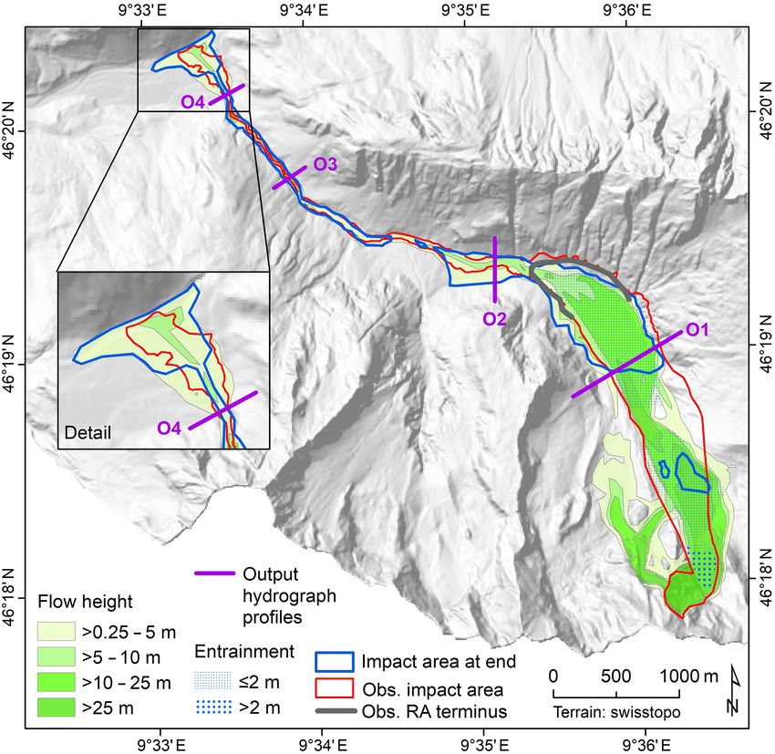
506                                  M. Mergili et al.: Back calculation of the 2017 Piz Cengalo–Bondo landslide cascade

tres away from the source and have led to major disasters in
the past, such as the 1949 Khait rock avalanche–loess flow
in Tajikistan (Evans et al., 2009b), the 1962 and 1970 Huas-
carán rockfall–debris avalanche events in Peru (Evans et al.,
2009a; Mergili et al., 2018b), the 2002 Kolka–Karmadon
ice–rock avalanche in Russia (Huggel et al., 2005), the 2012
Seti River debris flood in Nepal (Bhandari et al., 2012), or
the 2017 Piz Cengalo–Bondo rock avalanche–debris flow
event in Switzerland. The initial fall or slide sequences of
such process chains are commonly related to a changing
cryosphere characterized by glacial debuttressing, the forma-
tion of hanging glaciers, or a changing permafrost regime
(Harris et al., 2009; Krautblatter et al., 2013; Haeberli and
Whiteman, 2014; Haeberli et al., 2017).
   Computer models assist risk managers in anticipating the
impact areas, energies, and travel times of complex mass
flows. Conventional single-phase flow models, considering         Figure 1. Study area with the impact area of the 2017 Piz Cengalo–
                                                                  Bondo landslide cascade. The observed rock avalanche terminus
a mixture of solid and fluid components (e.g. Voellmy, 1955;
                                                                  was derived from WSL (2017).
Savage and Hutter, 1989; Iverson, 1997; McDougall and
Hungr, 2004; Christen et al., 2010), do not serve such a pur-
pose. Instead, simulations rely on the following:                 the documented and inferred impact areas, volumes, veloci-
  i. model cascades, changing from one approach to the            ties, and travel times. Based on the outcomes, we identify the
     next at each process boundary (Schneider et al., 2014;       key challenges to be addressed in future research.
     Somos-Valenzuela et al., 2016) so that each individual          As a result, we rely on the detailed description, doc-
     model is tailored for the corresponding process compo-       umentation, and topographic reconstruction of this recent
     nent,                                                        event. The event documentation, data used, and the concep-
                                                                  tual models are outlined in Sect. 2. We briefly introduce
 ii. bulk mixture models or two-phase or even multi-phase         the simulation framework r.avaflow (Sect. 3) and explain its
     flow models (Pitman and Le, 2005; Pudasaini, 2012;           parametrization and our simulation strategy (Sect. 4) before
     Iverson and George, 2014; Mergili et al., 2017; Pu-          presenting (Sect. 5) and discussing (Sect. 6) the results ob-
     dasaini and Mergili, 2019), since two-phase or multi-        tained. Finally, we conclude with the key messages of the
     phase flow models separately consider not only the solid     study (Sect. 7).
     and the fluid phase but also phase interactions and there-
     fore allow for considering more complex process inter-
     actions such as the impact of a landslide on a lake or       2     The 2017 Piz Cengalo–Bondo landslide cascade
     reservoir.
                                                                  2.1    Piz Cengalo and Val Bondasca
   Worni et al. (2014) have highlighted the advantages of the
second point for considering also the process interactions and    Val Bondasca is a left-tributary valley to Val Bregaglia in
boundaries.                                                       the canton of Grisons in southeastern Switzerland (Fig. 1).
   The aim of the present work is to learn about our abil-        The Bondasca stream joins the Mera River at the village of
ity to reproduce sophisticated transformation mechanisms          Bondo at 823 m a.s.l. It drains part of the Bregaglia Range,
involved in complex, cascading landslide processes with           built up by a mainly granitic intrusive body culminating
GIS-based tools. For this purpose, we apply the computa-          at 3678 m a.s.l. Piz Cengalo, with a summit elevation of
tional tool r.avaflow (Mergili et al., 2017), which employs       3368 m a.s.l., is characterized by a steep, intensely fractured
an enhanced version of the Pudasaini (2012) two-phase flow        northeastern face which has repeatedly been the scene of
model, to back calculate the 2017 Piz Cengalo–Bondo land-         landslides and which is geomorphologically connected to Val
slide cascade in southeastern Switzerland, which was char-        Bondasca through a steep glacier forefield. The glacier itself
acterized by the transformation of a rock avalanche to a          largely retreated to the cirque beneath the rock wall.
long-runout debris flow. We consider two scenarios in terms          On 27 December 2011, a rock avalanche with a volume of
of hypothetic qualitative conceptual models of the physical       1.5×10⁶ –2×10⁶ m3 developed out of a rock toppling from
transformation mechanisms. On this basis, we try to numer-        the northeastern face of Piz Cengalo, travelling for a dis-
ically reproduce these scenarios, satisfying the requirements     tance of 1.5 km down to the uppermost part of Val Bondasca
of physical plausibility of the model parameters and empiri-      (Haeberli, 2013; De Blasio and Crosta, 2016; Amann et al.,
cal adequacy in terms of correspondence of the results with       2018). This rock avalanche reached the main torrent channel.

Nat. Hazards Earth Syst. Sci., 20, 505–520, 2020                            www.nat-hazards-earth-syst-sci.net/20/505/2020/
M. Mergili et al.: Back calculation of the 2017 Piz Cengalo–Bondo landslide cascade                                             507

Figure 2. Oblique view of the impact area of the event from or-
thophoto draped over the 2011 DTM. Data sources: © swisstopo.

Erosion of the deposit thereafter resulted in increased debris
                                                                  Figure 3. The 2017 Piz Cengalo–Bondo landslide cascade.
flow activity (Frank et al., 2019). No entrainment of glacier     (a) Scarp area on 20 September 2014. (b) Scarp area on 23 Septem-
ice was documented for this event. As blue ice had been ob-       ber 2017 at 09:30 LT, 20 s after release, in frame of a video taken
served directly at the scarp, the role of permafrost for the      from the Capanna di Sciora. Note the fountain of water and/or
rock instability was discussed. An early warning system was       crushed ice at the front of the avalanche, most likely represent-
installed and later extended (Steinacher et al., 2018). Dis-      ing meltwater from the impacted glacier. (c) Upper part of Val
placements at the scarp area, measured by radar interferom-       Bondasca, where the channelized debris flow developed. Note the
etry and laser scanning, were a few centimetres per year be-      zone of dust- and pressure-induced damage to trees on the right
tween 2012 and 2015 and accelerated in the following years.       side of the valley. (d) Traces of the debris flows in Val Bon-
In early August 2017, increased rockfall activity and defor-      dasca. (e) The debris cone of Bondo after the event. Image sources:
                                                                  © Daniele Porro (a), © Diego Salasc/Reto and Barbara Salis (b),
mation rates alerted the authorities. A major rockfall event
                                                                  and © swisstopo (c–e).
occurred on 21 August 2017 (Amann et al., 2018).

2.2   The event of 23 August 2017
                                                                  tem which had been installed near the hamlet of Prä, ap-
The complex landslide which occurred on 23 August 2017            proximately 1 km upstream from Bondo. According to dif-
was documented mainly by reports of the Swiss Federal In-         ferent sources, the debris flow surge arrived at Bondo be-
stitute for Forest, Snow and Landscape Research (WSL); the        tween 09:42 (derived from WSL, 2017) and 09:48 LT (Amt
Laboratory of Hydraulics, Hydrology and Glaciology (VAW)          für Wald und Naturgefahren, 2017). The rather low velocity
of ETH Zurich; and the Amt für Wald und Naturgefahren             in the lower portion of Val Bondasca is most likely a con-
(Office for Forest and Natural Hazards) of the canton of          sequence of the narrow gorge topography and of the vis-
Grisons.                                                          cous behaviour of this first surge. Whereas approximately
   At 09:31 local time, a volume of approximately 3×10⁶ m3        540 000 m3 of material was involved, only 50 000 m3 arrived
detached from the northeastern face of Piz Cengalo, as in-        at Bondo immediately (data from the canton of Grisons; re-
dicated by WSL (2017), Amann et al. (2018), and the point         ported by WSL, 2017). The remaining material was partly
cloud we obtained through structure from motion (SfM) us-         remobilized by six further debris flow surges recorded dur-
ing pictures taken after the event. Documented by videos          ing the same day, one on 25 August, and one – triggered by
and by seismic records (Walter et al., 2018), it impacted the     rainfall – on 31 August 2017. All nine surges together de-
glacier beneath the rock face and entrained approximately         posited a volume of approximately 500 000–800 000 m3 in
6×10⁵ m3 of ice (VAW, 2017; WSL, 2017), was sharply de-           the area of Bondo, less than half of which was captured by a
flected at an opposite rock wall, and evolved into a rock (or     retention basin (Bonanomi and Keiser, 2017).
rock–ice) avalanche. Part of this avalanche immediately con-         The vertical profile of the main flow path is illustrated in
verted into a debris flow which flowed down Val Bondasca.         Fig. 4. The total angle of reach of the process chain from
It was detected at 09:34 LT by the debris flow warning sys-       the initial release down to the outlet of Val Bondasca was

www.nat-hazards-earth-syst-sci.net/20/505/2020/                             Nat. Hazards Earth Syst. Sci., 20, 505–520, 2020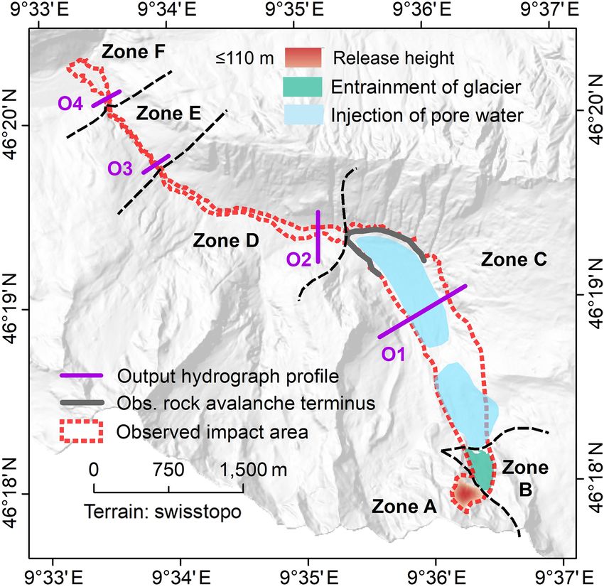
508                                   M. Mergili et al.: Back calculation of the 2017 Piz Cengalo–Bondo landslide cascade

approximately 17.4◦ , computed from the travel distance of        ering the water equivalent of the glacier ice) requires some
7.0 km and the vertical drop of approximately 2.2 km. The         spatio-temporal differentiation of the water and ice content.
initial landslide to the terminus of the rock avalanche showed    We consider two qualitative conceptual models – or scenar-
an angle of reach of approximately 25.8◦ , derived from the       ios – possibly explaining such a differentiation:
travel distance of 3.4 km and the vertical drop of 1.7 km. This
value is higher than the 22◦ predicted by the equation of          S1 The initial rockslide–rockfall led to massive entrain-
Scheidegger (1973), probably due to the sharp deflection of           ment fragmenting, and melting of glacier ice; mixing
the initial landslide. Following the concept of Nicoletti and         of rock with some of the entrained ice and the melt-
Sorriso-Valvo (1991), the rock avalanche was characterized            water, and injection of water from the basal sediments
by channelling of the mass. Only a limited run-up was ob-             into the rock avalanche mass quickly upon impact due to
served, probably due to the gentle horizontal curvature of the        overload-induced pore pressure rise. As a consequence,
valley in that area (no orthogonal impact on the valley slope;        the front of the rock avalanche was characterized by a
Hewitt, 2002). There were eight fatalities, concerning hikers         high content of ice and water, was highly mobile, and
in Val Bondasca, extensive damage to buildings and infras-            therefore escaped as the first debris flow surge, whereas
tructure, and evacuations for several weeks or even months.           the less mobile rock avalanche behind it – still with
                                                                      some water and ice in it – decelerated and deposited
2.3   Data and conceptual model                                       mid-valley. The secondary debris flow surges occurred
                                                                      mainly due to backwater effects. This scenario largely
Reconstruction of the rock and glacier volumes involved in            follows the explanation of Walter et al. (2020) in which
the event was based on an overlay of a 2011 swisstopo digital         the first debris flow surge was triggered at the front of
terrain model (DTM; contract: swisstopo–DV084371), de-                the rock avalanche by overload and pore pressure rise,
rived through airborne laser scanning in 2011 and available           whereas the later surges overtopped the rock avalanche
at a raster cell size of 2 m, and a digital surface model (DSM)       deposits, as indicated by the surficial scour patterns.
obtained through SfM techniques after the 2017 event. This
                                                                   S2 The initial rockslide–rockfall impacted and entrained
analysis resulted in a detached rock volume of 3.27×10⁶ m3 ,
                                                                      the glacier. Most of the entrained ice remained beneath
which is slightly more than the value of 3.15×10⁶ m3 re-
                                                                      the rock fragments and, after some initial sliding, de-
ported by Amann et al. (2018), and an entrained ice vol-
                                                                      veloped into an avalanching flow of melting ice behind
ume of 770 000 m3 (Fig. 5). However, these volumes neglect
                                                                      the rock avalanche. The rock avalanche decelerated and
smaller rockfalls before and after the large 2017 event and
                                                                      stopped mid-valley. Part of the avalanching flow over-
also glacial retreat. The 2011 event took place after the DTM
                                                                      topped and partly entrained the rock avalanche deposit
had been acquired, but it released from an area above the
                                                                      – leaving behind the scour traces observed in the field –
2017 scarp. The boundary between the 2011 and the 2017
                                                                      and evolved into the channelized debris flow which ar-
scarps, however, is slightly uncertain, which explains the dis-
                                                                      rived at Bondo a couple of minutes later. The secondary
crepancies between the different volume reconstructions. As-
                                                                      debris flow surges started from the rock avalanche de-
suming some minor entrainment of the glacier ice in 2011
                                                                      posit due to melting and infiltration of the remaining ice
and some glacial retreat, we arrive at an entrained ice vol-
                                                                      and due to backwater effects. This scenario is similar
ume of approximately 600 000 m3 , a value which is very well
                                                                      to the theory developed at the WSL Institute for Snow
supported by VAW (2017).
                                                                      and Avalanche Research (SLF), which also did a first
   There is still disagreement on the origin of the water that
                                                                      simulation of the rock avalanche (WSL, 2017).
led to the debris flow, particularly to the first surge. Bo-
nanomi and Keiser (2017) clearly mention meltwater from             Figure 6 illustrates the conceptual models attempting to
the entrained glacier ice as the main source, whereby much        explain the key mechanisms involved in the rock avalanche–
of the melting is assigned to impact, shearing, and frictional    debris flow transformation.
heating directly at or after impact, as is often the situation
in rock–ice avalanches (Pudasaini and Krautblatter, 2014).
WSL (2017) has shown, however, that the energy released           3   The simulation framework r.avaflow
was only sufficient to melt approximately half of the glacier
ice. Water pockets in the glacier or a stationary water source    r.avaflow represents a comprehensive GIS-based open-
along the path might have played an important role (Demmel,       source framework which can be applied for the simulation of
2019). Walter et al. (2020) claim that much of the glacier ice    various types of geomorphic mass flows. In contrast to most
was crushed, ejected, and dispersed (Fig. 3b), whereas water      other mass flow simulation tools, r.avaflow utilizes a general
injected into the rock avalanche due to pore pressure rise in     two-phase flow model describing the dynamics of the mix-
the basal sediments would have played a major role. In any        ture of solid particles and viscous fluid and the strong interac-
case, the development of a debris flow from a landslide mass      tions between these phases. It further considers erosion and
with an overall solid fraction of as high as ∼ 0.85 (consid-      entrainment of surface material along the flow path. These

Nat. Hazards Earth Syst. Sci., 20, 505–520, 2020                           www.nat-hazards-earth-syst-sci.net/20/505/2020/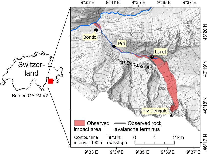
M. Mergili et al.: Back calculation of the 2017 Piz Cengalo–Bondo landslide cascade                                                     509

Figure 4. Profile along the main flow path of the Piz Cengalo–Bondo landslide cascade. The letters A–F indicate the individual zones (Table 1
and Fig. 7), whereas the associated numbers indicate the average angles of reach along the profile for each zone. The brown number and line
show the angle of reach of the initial landslide (rockslide–rockfall and rock – or rock—ice – avalanche), whereas the blue number and line
show the angle of reach of the entire landslide cascade. The geomorphic characteristics of the zone (in black) are indicated along with the
dominant process type (in green).

                                                                         ing from a defined release area (solid and/or fluid heights are
                                                                         assigned to each raster cell) or release hydrograph (at each
                                                                         time step, solid and/or fluid heights are added at a given pro-
                                                                         file, moving at a given cross-profile velocity) down through
                                                                         a DTM. The spatio-temporal evolution of the flow is approx-
                                                                         imated through depth-averaged solid and fluid mass and mo-
                                                                         mentum balance equations (Pudasaini, 2012). This system of
                                                                         equations is solved through the total-variation-diminishing
                                                                         (TVD) non-oscillatory central differencing (NOC) scheme
                                                                         introduced by Nessyahu and Tadmor (1990), adapting an ap-
                                                                         proach presented by Tai et al. (2002) and Wang et al. (2004).
                                                                         The characteristics of the simulated flow are governed by a
                                                                         set of flow parameters (some of them are shown in the Ta-
                                                                         bles 1 and 2).
                                                                            The solid and fluid phases have their own mass and mo-
                                                                         mentum balance equations so that they evolve as independent
Figure 5. Reconstruction of the released rock volume and the en-
                                                                         dynamical quantities while the phases are still coupled. This
trained glacier volume in the 2017 Piz Cengalo–Bondo landslide
                                                                         means that, in general, the solid and fluid velocities are differ-
cascade. Note that the boundary between the 2011 and 2017 re-
lease volumes is connected to some uncertainties, explaining the         ent. However, the use of an enhanced drag model (Pudasaini,
slight discrepancies among the reported volumes. The glacier vol-        2019) and the consideration of virtual mass forces ensure
ume shown is neither corrected for entrainment related to the 2011       a strong coupling between the solid and the fluid phases in
event nor for glacier retreat in the period 2011–2017.                   the mixture (Pudasaini, 2012; Pudasaini and Mergili, 2019).
                                                                         Compared to the Pudasaini (2012) model, some further ex-
                                                                         tensions have been introduced which include (i) ambient drag
                                                                         or air resistance (Kattel et al., 2016; Mergili et al., 2017) and
features facilitate the simulation of cascading landslide pro-           (ii) fluid friction, governing the influence of basal surface
cesses such as the 2017 Piz Cengalo–Bondo event. r.avaflow               roughness on the fluid momentum (Mergili et al., 2018b).
is outlined in full detail by Mergili and Pudasaini (2019).              Both extensions rely on empirical coefficients, CAD for the
The code, a user manual, and a collection of test datasets               ambient drag and CFF for the fluid friction. Further, viscosity
are available from Mergili and Pudasaini (2019). Only the                is computed according to an improved concept. As in Dom-
aspects directly relevant to the present work are described in           nik et al. (2013) and Pudasaini and Mergili (2019), the fluid
this section.                                                            viscosity is enhanced by the yield strength. Most importantly,
   Essentially, the Pudasaini (2012) two-phase flow model is             the internal friction angle ϕ and the basal friction angle δ of
employed for computing the dynamics of mass flows mov-

www.nat-hazards-earth-syst-sci.net/20/505/2020/                                    Nat. Hazards Earth Syst. Sci., 20, 505–520, 2020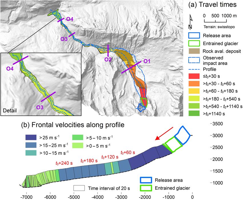
510                                             M. Mergili et al.: Back calculation of the 2017 Piz Cengalo–Bondo landslide cascade

Table 1. Descriptions and optimized parameter values for each of the zones A–F (Figs. 4 and 7). The names of the model parameters are given
in the text and in Table 2. The values provided in Table 2 are assigned to those parameters not shown. S1 and S2 refer to the corresponding
scenarios.

                     Zone        Description                                    Model parameters                Initial conditions
                     A           Rock zone – northeastern face                  δ = 20◦ (S1)a                   Release volume:
                                 of Piz                                         δ = 13◦ (S2)b                   3.2×10⁶ m3 , 100 % solidc
                                 Cengalo      with  rockslide–                  CAD = 0.2
                                 rockfall
                                 release area
                     B           Glacier zone – cirque glacier                  δ = 20◦ (S1)                    Entrainment of glacier ice and
                                 beneath zone A, entrainment of                 δ = 13◦ (S2)                    till (Table 3)d
                                 glacier icea                                   CE = 10−6.5
                     C           Slope zone – steep, partly                     δ = 20◦ (S1)                    Entrainment of injected water
                                 debris-covered glacier forefield               δ = 13◦ (S2)                    in Scenario S1
                                 leading down to Val                            CE = 10−6.5 (S1)                Entrainment of rock avalanche
                                 Bondasca                                       CE = 10−8.0 (S2)                deposit in Scenario S2
                     D           Upper Val Bondasca zone –                      δ = 20–45◦                      No entrainment allowed,
                                 clearly defined flow channel                                                   increasing friction
                                 becoming narrower in
                                 downstream direction
                     E           Lower Val Bondasca zone –                      δ = 45◦                         No entrainment allowed, high
                                 narrow gorge                                   CFF = 0.5                       friction due to lateral confine-
                                                                                                                ment
                     F           Bondo zone – deposition of                     δ = 20◦                         No entrainment allowed
                                 the debris flow on the cone of
                                 Bondo
                   a Note that in all zones and in both of the scenarios, S1 and S2, δ is assumed to scale linearly with the solid fraction. This means
                   that the values given only apply in case of 100 % solid material. b This only applies to the initial landslide, which is assumed
                   completely dry in Scenario S2. Due to the scaling of δ with the solid fraction, a lower basal friction is required to obtain results
                   similar to Scenario S1, where the rock avalanche contains some fluid. The same values of δ as for Scenario S1 are applied for the
                   debris flow in Scenario S2 throughout all zones. c This volume is derived from our own reconstruction (Fig. 5). In contrast, WSL
                   (2017) gives 3.1×10⁶ m3 and Amann et al. (2018) 3.15×10⁶ m3 . d In Scenario S2, the glacier is not directly entrained but instead
                   released behind the rock avalanche. In both scenarios, ice is considered to melt immediately on impact and included in the viscous
                   fluid fraction. See text for more detailed explanations.

Table 2. Model parameters used for the simulations.

                           Symbol         Parameter                                              Unit           Value
                           ρS             Solid material density (grain density)                 kg m−3         2700
                           ρF             Fluid material density                                 kg m−3         1400a
                           ϕ              Internal friction angle                                Degree         27b
                           δ              Basal friction angle                                   Degree         Table 1
                           ν              Kinematic viscosity of the fluid                       m2 s−1         10
                           τY             Yield strength of the fluid                            Pa             10
                           CAD            Ambient drag coefficient                               –              0.04 (exceptions in Table 1)
                           CFF            Fluid friction coefficient                                            0.0 (exceptions in Table 1)
                           CE             Entrainment coefficient                                –              Table 1
                         a Fluid is considered here to be a mixture of water and fine particles. This explains the higher density compared to pure
                         water. b The internal friction angle ϕ always has to be larger than or equal to the basal friction angle δ . Therefore, in the
                         case of δ>ϕ , ϕ is increased accordingly.

Nat. Hazards Earth Syst. Sci., 20, 505–520, 2020                                                         www.nat-hazards-earth-syst-sci.net/20/505/2020/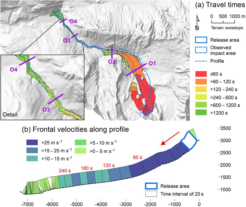
M. Mergili et al.: Back calculation of the 2017 Piz Cengalo–Bondo landslide cascade                                                    511

Figure 6. Qualitative conceptual models of the rock avalanche–debris flow transformation. (a) Scenario S1. (b) Scenario S2. See text for the
detailed description of the two scenarios.

the solid are scaled with the solid fraction in order to ap-            sequent surges or distal debris floods beyond Bondo are con-
proximate effects of reduced interaction between the solid              sidered in this study. Equally, the dust cloud associated to the
particles and the basal surface in fluid-rich flows.                    rock avalanche (WSL, 2017) is not the subject here. Initial
   Entrainment is calculated through an empirical model.                sliding of the glacier beneath the rock avalanche, as assumed
In contrast to Mergili et al. (2017), where an empiri-                  in Scenario S2, cannot directly be modelled. That would re-
cal entrainment coefficient is multiplied by the momentum               quire a three-phase model, which is beyond the scope here.
of the flow, here we multiply the entrainment coefficient               Instead, release of the glacier ice and meltwater is assumed
CE (s kg−1 m−1 ) by the kinetic energy of the flow:                     in a separate simulation after the rock avalanche has passed
                                                                       over it. We consider this workaround an acceptable approxi-
qE,s = CE |Ts + Tf | αs,E , qE,f = CE |Ts + Tf | 1 − αs,E , (1)         mation of the postulated scenario (Sect. 6).
                                                                           We use the 2011 swisstopo DTM, corrected for the
where qE,s and qE,f (m s−1 ) are the solid and fluid entrain-
                                                                        rockslide–rockfall scarp and the entrained glacier ice by
ment rates, Ts and Tf (J) are the kinetic energies of the solid
                                                                        overlay with the 2017 SfM DSM (Sect. 2). The maps of
and fluid fractions of the flow, and αs,E is the solid fraction of
                                                                        release height and maximum entrainable height are derived
the entrainable material. Solid and fluid flow heights and mo-
                                                                        from the difference between the 2011 swisstopo DTM and
menta, and the change of the basal topography, are updated
                                                                        the 2017 SfM DSM (Fig. 5; Sect. 2). The release mass is
at each time step (see Mergili et al., 2017, for details).
                                                                        considered completely solid, whereas the entrained glacier
   As r.avaflow operates on the basis of GIS raster cells, its
                                                                        is assumed to contain some solid fraction (coarse till). The
output essentially consists of raster maps – for all time steps
                                                                        glacier ice is assumed to melt immediately on impact and is
and for the overall maximum – of solid and fluid flow heights,
                                                                        included in the fluid along with fine till. We note that the fluid
velocities, pressures, kinetic energies, and entrained heights.
                                                                        phase does not represent pure water but rather a mixture of
In addition, output hydrograph profiles may be defined by
                                                                        water and fine particles (Table 2). The fraction of the glacier
which solid and fluid heights, velocities, and discharges are
                                                                        allowed to be incorporated in the process chain is empiri-
provided at each time step.
                                                                        cally optimized (Table 3). Based on the same principle, the
                                                                        maximum depth of entrainment of fluid due to pore pressure
4   Parameterization of r.avaflow                                       overload in Scenario S1 is set to 25 cm, whereas the maxi-
                                                                        mum depth of entrainment of the rock avalanche deposit in
One set of simulations is performed for each of the scenarios,          Scenario S2 is set to 1.5 m.
S1 and S2 (Fig. 6), considering the process chain from the re-             The study area is divided into six zones, labelled A–F
lease of the rockslide–rockfall to the arrival of the first debris      (Figs. 4 and 7; Table 1). Each of these zones represents an
flow surge at Bondo. Neither triggering of the event nor sub-           area with particular geomorphic characteristics and domi-

www.nat-hazards-earth-syst-sci.net/20/505/2020/                                    Nat. Hazards Earth Syst. Sci., 20, 505–520, 2020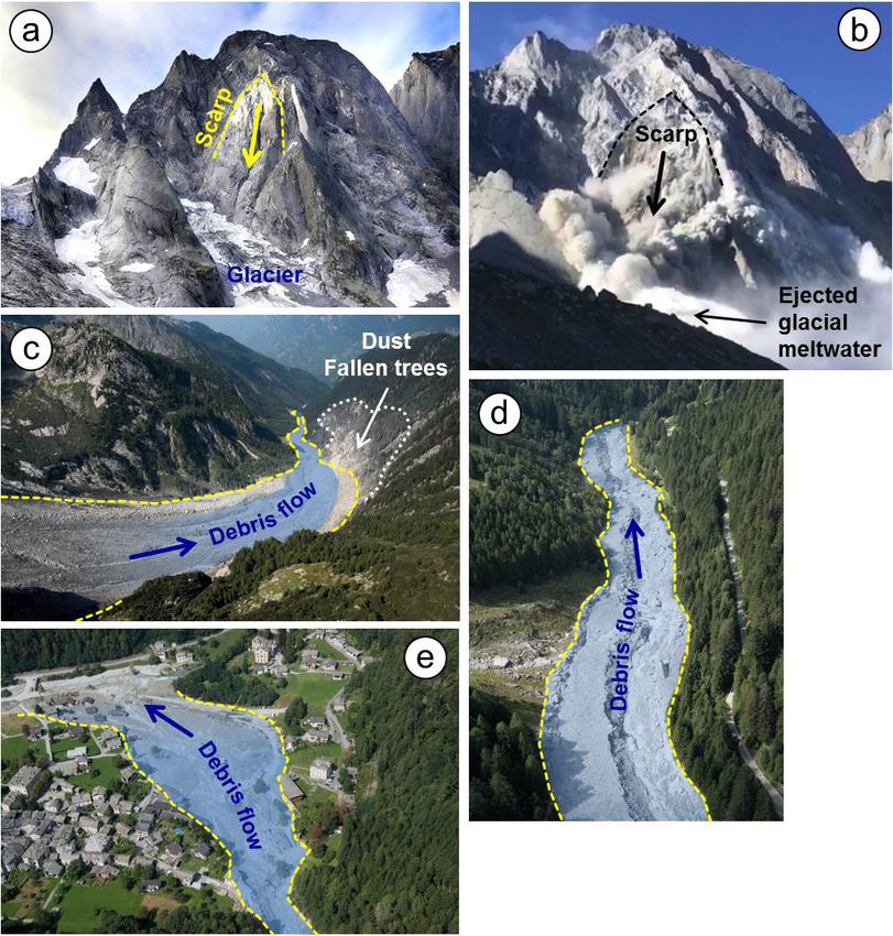
512                                               M. Mergili et al.: Back calculation of the 2017 Piz Cengalo–Bondo landslide cascade

Table 3. Selected output parameters of the simulations for the scenarios S1 and S2 compared to the observed or documented parameter
values. S is solid, F is fluid, fractions are expressed in terms of volume, and t0 is time from the initial release to the release of the first
debris flow surge. Reference values are extracted from Amt für Wald und Naturgefahren (2017), Bonanomi and Keiser (2017), and WSL
(2017). *** is empirically adequate (within the documented range of values). ** is empirically partly adequate (less than 50 % away from the
documented range of values). * is empirically inadequate (at least 50 % away from the documented range of values). The arithmetic means
of minimum and maximum of each range are used for the calculations.

              Parameter                                     Documentation and observation                             Scenario S1                    Scenario S2
              Entrained ice (m3 )                                                          600 000a                          –                              –
              Entrained S (m3 )                                                                   –                     60 000                        60 000b
              Entrained F (m3 )                                                                   –                    305 000                        240 000
              Duration of initial landslide (s)                                             60–90c                 100–120**                       100–120**
              Travel time to O2 (s)                                                        90–120d                      140**                     t0 + 120***
              Travel time to O3 (s)                                                       210–300e                     280***                     t0 + 240***
              Travel time to O4 (s)                                                      630–1020f                     700***                     t0 + 640***
              Debris flow volume at O2 (m3 )                                                540 000         530 000** (43 % S)             430 000** (45 % S)
              Debris flow volume at O4 (m3 )                                                 50 000          265 000* (34 % S)              270 000* (24 % S)
            a Not all the material entrained from the glacier was relevant to the first debris flow surge (Fig. 6); therefore lower volumes of entrained S (coarse till;
            in Scenario S2 also rock avalanche deposit) and F (molten ice and fine till; in Scenario S1 also pore water) yield the empirically most adequate
            results. The F volumes originating from the glacier in the simulations represent approximately half of the water equivalent of the entrained ice,
            corresponding well to the findings of WSL (2017). b This value does not include the 145 000 m3 of solid material remobilized through entrainment
            from the rock avalanche deposit in Scenario S2. c WSL (2017) states that the rock avalanche came to rest approximately 60 s after release, whereas
            the seismic signals ceased 90 s after release. d A certain time (here, we assume a maximum of 30 s) has to be allowed for the initial debris flow surge
            to reach O2, located slightly downstream of the front of the rock avalanche deposit. e WSL (2017) gives a travel time of 3.5 min to Prä, roughly
            corresponding to the location of O3. It remains unclear whether this number refers to the release of the initial rockslide–rockfall or (more likely) to
            the start of the first debris flow surge. Bonanomi and Keiser (2017) give a travel time of roughly 4 min between the initial release and the arrival of
            the first surge at the sensor of Prä. f Amt für Wald und Naturgefahren (2017) gives a time span of 17 min between the release of the initial
            rockslide–rockfall and the arrival of the first debris flow surge at the “bridge” in Bondo. However, the bridge that this number refers to is not
            indicated. WSL (2017), in contrast, gives a travel time of 7–8 min from Prä to the “old bridge” in Bondo, which, in sum, results in a shorter total
            travel time as indicated in Amt für Wald und Naturgefahren (2017). Depending on the bridge, the reference location for these numbers might be
            downstream from O4. In the simulation, this hydrograph shows a slow onset – travel times refer to the point when 5 % of the total peak discharge is
            reached.

nant process types, which can be translated into model pa-                                   linearly with the solid fraction – this means that the values
rameters. Due to the impossibility of directly measuring the                                 given in Table 1 only apply for 100 % solid material.
key parameters in the field (Mergili et al., 2018a, b), the                                     Durations of t = 1800 s are considered for both scenarios.
parameters summarized in Tables 1 and 2 are the result of                                    At this point in time, the first debris flow surge largely passed
an iterative optimization procedure, where multiple simula-                                  and left the area of interest, except for some remaining tail
tions with different parameter sets are performed in order                                   of fluid material. Only heights ≥ 0.25 m are taken into ac-
to arrive at one “optimum” simulation for each scenario. It                                  count for the visualization and evaluation of the simulation
is thereby important to note that we largely derive one sin-                                 results. A threshold of 0.001 m is used for the simulation
gle set of optimized parameters which is valid for both of                                   itself, keeping the loss due to numerical diffusion within a
the scenarios. Optimization criteria are (i) the empirical ad-                               range of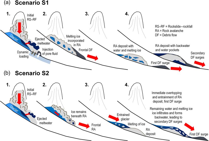
M. Mergili et al.: Back calculation of the 2017 Piz Cengalo–Bondo landslide cascade 513
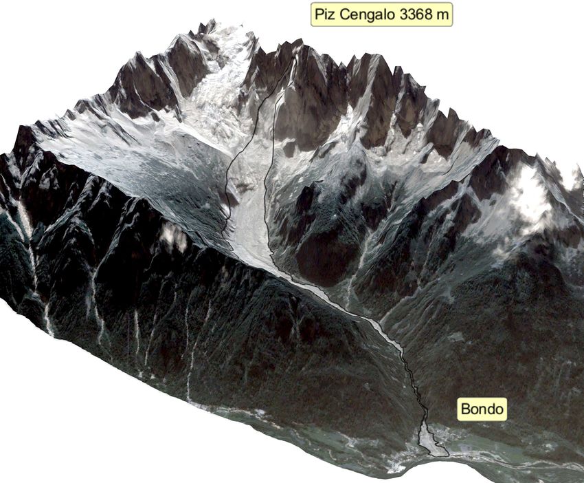
Figure 7. Overview of the heights and entrainment areas as well Figure 8. Maximum flow height and entrainment derived for Sce-
as the zonation performed as the basis for the simulation with nario S1. RA is rock avalanche; the observed RA terminus was de-
r.avaflow. Injection of pore water only applies to Scenario A. The rived from WSL (2017).
zones A–F represent areas with largely homogeneous surface char-
acteristics. The characteristics of the zones and the model parame-
ters associated to each zone are summarized in Table 1 and Fig. 4.
O1–O4 represent the output hydrograph profiles. The observed rock
increases to around 3 m and remains so until the end of the
avalanche terminus was derived from WSL (2017).
simulation, whereas the fluid flow height slowly and steadily
tails off. Until t = 1800 s the profile O2 is passed by a to-
tal of 221 000 m3 of solid and 308 000 m3 of fluid material
lated impact areas results in a critical success index (CSI) of (the fluid representing a mixture of fine mud and water with
0.558, a distance to perfect classification (D2PC) of 0.167, a density of 1400 kg m−3 ; see Table 2). The hydrograph pro-
and a factor of conservativeness (FoC) of 1.455. These per- file O3 in Prä, approximately 1 km upstream of Bondo, is
formance indicators are derived from the confusion matrix of characterized by a surge starting before t = 280 s and slowly
true positives, true negatives, false positives, and false nega- tailing off afterwards. Discharge at the hydrograph OH4
tives. CSI and D2PC measure the correspondence of the ob- (Fig. 9b; O4 is located at the outlet of the canyon to the de-
served and simulated impact areas. Both indicators can range bris fan of Bondo) starts at around t = 700 and reaches its
between 0 and 1, whereby values of CSI close to 1 and values peak of solid discharge at t = 1020 s (167 m3 s−1 ). Solid dis-
of D2PC close to 0 point to a good correspondence. FoC in- charge decreases thereafter, whereas the flow becomes fluid-
dicates whether the observed impact areas are overestimated dominated with a fluid peak of 202 m3 s−1 at t = 1320 s. The
(FoC > 1) or underestimated by the simulation (FoC < 1). maximum total flow height simulated at O4 is 2.53 m. This
More details are provided by Formetta et al. (2016) and by site is passed by a total of 91 000 m3 of solid and 175 000 m3
Mergili et al. (2017, 2018a). of fluid material, according to the simulation – an overesti-
Interpreting these values as indicators for a reasonably mate, compared to the documentation (Table 3).
good correspondence between simulation and observation in Figure 10 illustrates the travel times and the frontal veloc-
terms of impact area, we now consider the dimension of time, ities of the rock avalanche and the initial debris flow. The ini-
focussing on the output hydrographs OH1–OH4 (Fig. 9; see tial surge reaches the hydrograph profile O3 – located 1 km
Figs. 7 and 8 for the location of the corresponding hydro- upstream of Bondo – at t = 280 s (Fig. 10a; Fig. 9c). This is
graph profiles O1–O4). Much of the rock avalanche passes in line with the documented arrival of the surge at the nearby
the profile O1 between t = 60 s and t = 100 s. OH2 (Fig. 9a; monitoring station (Table 3). Also the simulated travel time
located in the upper portion of Val Bondasca) sets on be- to the profile O4 corresponds to the existing – though uncer-
fore t = 140 s and quickly reaches its peak, with a volumet- tain – documentation. The initial rock avalanche is character-
ric solid ratio of approximately 30 % (maximum 900 m3 s−1 ized by frontal velocities >25 m s−1 , whereas the debris flow
of solid and 2200 m3 s−1 of fluid discharge). Thereafter, this largely moves at 10–25 m s−1 . Velocities drop below 5 m s−1
first surge quickly tails off. The solid flow height, however, in the lower part of the valley (Zone E; Fig. 10b).
www.nat-hazards-earth-syst-sci.net/20/505/2020/ Nat. Hazards Earth Syst. Sci., 20, 505–520, 2020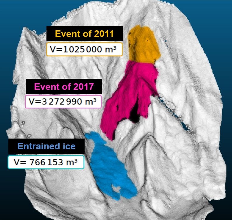
514                                      M. Mergili et al.: Back calculation of the 2017 Piz Cengalo–Bondo landslide cascade

Figure 9. Output hydrographs OH2 and OH4 derived for the scenarios S1 and S2. (a) OH2 for Scenario S1. (b) OH4 for Scenario S1. (c)
OH2 for Scenario S2. (d) OH4 for Scenario S2. See Figs. 7 and 8 for the locations of the hydrograph profiles O2 and O4. Hs is solid flow
height, Hf is fluid flow height, Qs is solid discharge, and Qf is fluid discharge.

                                                                        5.2   Scenario S2 – debris flow surge by overtopping and
                                                                              entrainment of rock avalanche

                                                                        Figure 11 illustrates the distribution of the simulated maxi-
                                                                        mum flow heights, maximum entrained heights, and deposi-
                                                                        tion area after t = t0 + 1740 s, where t0 is the time between
                                                                        the release of the initial rock avalanche and the mobiliza-
                                                                        tion of the entrained glacier. The simulated impact and de-
                                                                        position areas of the initial rock avalanche are also shown
                                                                        in Fig. 11. However, we now concentrate on the debris flow,
                                                                        triggered by the simulated entrainment of 145 000 m3 of solid
                                                                        material from the rock avalanche deposit. Flow heights – as
                                                                        well as the hydrographs presented in Fig. 9c and d and the
                                                                        temporal patterns illustrated in Fig. 12 – only refer to the
                                                                        debris flow developing from the entrained glacier and the
                                                                        entrained rock avalanche material. The confusion matrix of
                                                                        observed and simulated impact areas reveals partly different
                                                                        patterns of performance than for Scenario S1: CSI = 0.590,
Figure 10. Spatio-temporal evolution and velocities of the event
                                                                        D2PC = 0.289, and FoC = 0.925. The lower FoC value and
obtained for Scenario S1. (a) Travel times, starting from the re-
lease of the initial rockslide–rockfall. (b) Frontal velocities along   the lower performance in terms of D2PC reflect the miss-
the flow path, shown in steps of 20 s. Note that the height of the      ing initial rock avalanche in the simulation results. The out-
velocity graph does not scale with flow height. White areas indicate    put hydrographs OH2 and OH4 differ from the hydrographs
that there is no clear flow path.                                       obtained through Scenario S1 but also show some similari-
                                                                        ties (Fig. 9c and d). Most of the flow passes through the hy-
                                                                        drograph profile O1 between t = t0 + 40 s and t0 + 80 s and
                                                                        through O2 between t = t0 +100 s and t0 +180 s. The hydro-
                                                                        graph OH2 is characterized by a short peak of 3500 m3 s−1
                                                                        of solid and 4500 m3 s−1 of fluid material, with a volumet-
                                                                        ric solid fraction of 0.44, and quickly decreasing discharge

Nat. Hazards Earth Syst. Sci., 20, 505–520, 2020                                 www.nat-hazards-earth-syst-sci.net/20/505/2020/
M. Mergili et al.: Back calculation of the 2017 Piz Cengalo–Bondo landslide cascade 515
Figure 12. Spatio-temporal evolution and velocities of the event ob-
tained for Scenario S2. (a) Travel times, starting from the release of
the initial rockslide–rockfall. Therefore t0 (s) is the time between
Figure 11. Maximum flow height and entrainment derived for Sce- the release of the rockslide–rockfall and the mobilization of the en-
nario S2. RA is rock avalanche; the observed RA terminus was de- trained glacier. (b) Frontal velocities along the flow path, shown in
rived from WSL (2017). steps of 20 s. Note that the height of the velocity graph does not
scale with flow height. White areas indicate that there is no clear
flow path.
afterwards (Fig. 9c). In contrast to Scenario S1, flow heights
of CE and the allowed height of entrainment chosen for the
drop steadily, with values below 2 m from t = t0 + 620 s on-
rock avalanche deposit.
wards. The hydrograph OH3 is characterized by a surge start-
ing around t = t0 + 240 s. Discharge at the hydrograph OH4
(Fig. 9d) sets at around t = t0 + 600 s, and the solid peak 6 Discussion
of 240 m3 s−1 is simulated at approximately t = t0 + 780 s.
The delay of the peak of fluid discharge is more pronounced Our simulation results reveal a reasonable degree of empiri-
when compared to Scenario S1 (310 m3 s−1 at t = t0 +960 s). cal adequacy and physical plausibility with regard to most of
Profile O4 is passed by a total of 65 000 m3 of solid and the reference observations. Having said that, we have also
204 000 m3 of fluid material. The volumetric solid fraction identified some important limitations which are now dis-
drops from above 0.60 at the very onset of the hydrograph cussed in more detail. First of all, we are not able to decide on
to around 0.10 (almost pure fluid) at the end. The maximum the more realistic of the two scenarios, S1 and S2. In general,
total flow height at O4 is 3.1 m. the melting and mobilization of glacier ice upon rockslide–
Figure 12 illustrates the travel times and the frontal ve- rockfall impact are hard to quantify from straightforward cal-
locities of the rock avalanche and the initial debris flow. As- culations of energy transformation, as Huggel et al. (2005)
suming that t0 is in the range of some tens of seconds, the have demonstrated on the example of the 2002 Kolka–
time of arrival of the surge at O3 is in line with the documen- Karmadon event. In the present work, the assumed amount
tation also for Scenario S2 (Fig. 12a; Table 3). The frontal of melting (approximately half of the glacier ice) leading
velocity patterns along Val Bondasca are roughly in line with to the empirically most adequate results corresponds well
those derived in Scenario S1 (Fig. 12b). However, the sce- to the findings of WSL (2017), indicating a reasonable de-
narios differ among themselves in terms of the more pro- gree of plausibility. It remains equally difficult to quantify
nounced but shorter peaks of the hydrographs in Scenario S2 the amount of water injected into the rock avalanche by over-
(Fig. 9). This pattern is a consequence of the more sharply load of the sediments and the resulting pore pressure rise
defined debris flow surge. In Scenario S1, the front of the (Walter et al., 2020). Confirmation or rejection of conceptual
rock avalanche deposit constantly releases material into Val models with regard to the physical mechanisms involved in
Bondasca, providing supply for the debris flow also at later specific cases would have to be based on better-constrained
stages. In Scenario S2, entrainment of the rock avalanche de- initial conditions and the availability of robust parameter
posit occurs relatively quickly, without material supply after- sets.
wards. This type of behaviour is strongly coupled to the value
www.nat-hazards-earth-syst-sci.net/20/505/2020/ Nat. Hazards Earth Syst. Sci., 20, 505–520, 2020516 M. Mergili et al.: Back calculation of the 2017 Piz Cengalo–Bondo landslide cascade We note that with the approach chosen we are not able how arbitrary. The elaboration of well-suited stopping crite- (i) to adequately simulate the transition from solid to fluid ria, going beyond the very simple approach introduced by material and (ii) to consider rock and ice separately with dif- Mergili et al. (2017), remains a task for the future. How- ferent material properties, which would require a three-phase ever, as the rock avalanche has already been successfully model and is thus not within the scope here. Therefore, en- back calculated by WSL (2017), we focus on the first de- trained ice is considered viscous fluid from the beginning. A bris flow surge: the simulation input is optimized towards the physically better-founded representation of the initial phase back calculation of the debris flow volumes entering the val- of the event would require an extension of the flow model ley at the hydrograph profile O2 (Table 3). The travel times employed. Such an extension could build on the rock–ice to the hydrograph profiles O3 and O4 are reproduced in a avalanche model introduced by Pudasaini and Krautblatter plausible way in both scenarios, and so are the impact ar- (2014). Also, the vertical patterns of the situation illustrated eas (Figs. 8 and 11). Exceedance of the lateral limits in the in Fig. 5 cannot be modelled with the present approach, lower zones is attributed to an overestimate of the debris flow which (i) does not consider melting of ice and (ii) only al- volumes there and to numerical issues related to the narrow lows one entrainable layer at each pixel. The assumption of gorge: the steep walls of the gorge, in combination with the fluid behaviour of entrained glacier ice therefore represents a low number of raster cells representing the width of the flow, necessary simplification which is supported by observations challenge the correct geometric representation of the flow in (Fig. 3b) but neglects the likely presence of remaining ice in the topography-following coordinate system. Further, appli- the basal part of the eroded glacier, which melted later and cation of the TVD NOC scheme results in numerical dif- so contributed to the successive debris flow surges. fusion which becomes particularly evident in this situation. Still, we currently consider the Pudasaini (2012) model – The introduction of adaptive meshes – which would help to and the extended multi-phase model (Pudasaini and Mergili, locally increase the spatial resolution while maintaining the 2019) – to be best practice, even though other two-phase or computational efficiency – could alleviate this type of issue bulk mixture models do exist. Most recently, Iverson and in the future. The same is true for the fan of Bondo. The George (2014) presented an approach that has been solved solid ratio of the debris flow in the simulations appears re- with an open-source software, called D-Claw (George and alistic, ranging from around 40 % to 45 % in the upper part Iverson, 2014), and compared it to large-scale experiments of the debris flow path and from around 30 % to 35 % and considering dense debris materials (Iverson et al., 2000, lower (depending on the cut-off time of the hydrograph) in 2010). The Iverson and George (2014) model can be use- the lower part. This means that solid material tends to stop in ful for flow-type landslides, or bulk motion, where the solid the transit area rather than fluid material, as can be expected. particles and fluid molecules move together. However, the Nevertheless, the correct simulation of the deposition of de- Pudasaini (2012) model is better suited for the simulation of bris flow material along Val Bondasca remains a major chal- cascading mass flows for the following reasons: (i) solid and lenge (Table 3). Even though a considerable amount of effort fluid velocities are considered separately, which is important was put into reproducing the much lower volumes reported for complex, cascading mass flows; (ii) pore fluid diffusion is in the vicinity of O4, the simulations result in an overesti- included, whereas the model of Iverson and George (2014) is mate of the volumes passing through this hydrograph profile. limited to pore pressure advection and source terms associ- This is most likely a consequence of the failure of r.avaflow ated with dilation; (iii) interfacial momentum transfers, such to adequately reproduce the deposition pattern in the zones as the drag force, virtual mass force, and buoyancy between D and E. Whereas some material remains there at the end the solid and fluid phases are fully included; and (iv) vis- of the simulation, more work is necessary to appropriately cous shear stress and dynamical coupling between the pore understand the mechanisms of deposition in viscous debris fluid pressure evolution and the bulk momentum equations flows (Pudasaini and Fischer, 2016). Part of the discrepancy, are considered. however, might be explained by the fact that part of the fluid The initial rockslide–rockfall and the rock avalanche are material – which does not only consist of pure water but also simulated in a plausible way, at least with regard to the depo- consists of a mixture of water and fine mud – left the area sition area. Whereas the simulated deposition area is clearly of interest in the downstream direction and was therefore not defined in Scenario S2, this is to a lesser extent the case included in the reference measurements. That lower part of in Scenario S1, where the front of the rock avalanche di- the process chain was not subject of the present work. rectly transforms into a debris flow. Both scenarios seem to The simulation results are strongly influenced by the ini- overestimate the time between release and deposition com- tial conditions and the model parameters. Parameterization pared to the seismic signals recorded – an issue also re- of both scenarios is complex and highly uncertain, particu- ported by WSL (2017) for their simulation. We observe a larly in terms of optimizing the volumes of entrained till and relatively gradual deceleration of the simulated avalanche, glacial meltwater and injected pore water. In general, the pa- without clearly defined stopping, and note that also in Sce- rameter sets optimized to yield empirically adequate results nario S2, there is some diffusion after the considered time of are physically plausible. Reproducing the travel times to O4 120 s so that the definition of the simulated deposit is some- in the present study requires the assumption of a low mobility Nat. Hazards Earth Syst. Sci., 20, 505–520, 2020 www.nat-hazards-earth-syst-sci.net/20/505/2020/
M. Mergili et al.: Back calculation of the 2017 Piz Cengalo–Bondo landslide cascade                                               517

of the flow in Zone E. This is achieved by increasing the fric-    of the scope of the present work. Therefore, we have used a
tion (Table 1), accounting for the narrow flow channel, i.e.       stepwise expert-based optimization strategy.
the interaction of the flow with the channel walls, which is
not directly accounted for in r.avaflow. Still, the high values
of δ given in Table 1 are not directly applied, as they scale
                                                                   7   Conclusions
with the solid fraction. This type of weighting has to be fur-
ther scrutinized. We emphasize that also reasonable parame-        We have back calculated the 2017 Piz Cengalo–Bondo land-
ter sets are not necessarily physically true, as the large num-
                                                                   slide cascade in Switzerland, where an initial rockslide–
ber of parameters involved (Tables 1 and 2) create a lot of
                                                                   rockfall of approximately 3×10⁶ m3 entrained a glacier, con-
space for equifinality issues (Beven et al., 1996). The higher
                                                                   tinued as a rock avalanche, and finally converted into a series
values of δ in the lower portion of the channel are based on       of debris flows, reaching the village of Bondo at a total dis-
the assumption that δ of the solid material would somehow          tance of 6.5 km. The water causing the transformation into
depend on the momentum or energy of the flow, which – due          a debris flow might have originated from entrained glacier
to the relatively low velocity – is much less in the zones D
                                                                   ice or from water injected from the debris beneath the rock
and, particularly, E. While this assumption, in our opinion, is
                                                                   avalanche. Considering the event from its initiation to the
justified by fluidization and lubrication effects often observed
                                                                   first debris flow surge, we have evaluated not only the possi-
– or inferred – for very rapid mass flows, it remains hard to      bilities but also the challenges in the simulation of such com-
consider those effects by a well-justified numerical relation-     plex landslide events, employing the two-phase model of the
ship. Until such a relationship (which definitely remains an       software r.avaflow.
important subject of future work) has been proposed, we rely
                                                                      Both of the investigated scenarios, S1 (debris flow de-
on empirically based zonation of friction parameters.
                                                                   veloping through injected water at the front of the rock
   We have further shown that the classical evaluation of em-
                                                                   avalanche) and S2 (debris flow developing through melted
pirical adequacy, by comparing observed and simulated im-          ice at the back of the rock avalanche, overtopping the de-
pact areas, is insufficient in the case of complex mass flows:     posit), lead to empirically reasonably adequate results when
travel times, hydrographs, and volumes involved can provide
                                                                   back calculated with r.avaflow using physically plausible
important insight in addition to the quantitative performance
                                                                   model parameters. Based on the simulations performed in
indicators used, for example, in landslide susceptibility mod-
                                                                   the present study, final conclusions on the more likely of the
elling (Formetta et al., 2016). Further, the delineation of the
                                                                   mechanisms sketched in Fig. 6 can therefore not be drawn
observed impact area is uncertain, as the boundary of the          purely based on the simulations. The observed jet of glacial
event is not clearly defined particularly in Zone C. Also,         meltwater (Fig. 3b) points towards Scenario S1. The ob-
the other reference data are not exact. Therefore, we allow
                                                                   served scouring of the rock avalanche deposit, in contrast,
a broad margin (50 % deviation of the observation) for con-
                                                                   rather points towards Scenario S2 but could also be asso-
sidering the model outcomes as empirically adequate.
                                                                   ciated to subsequent debris flow surges. Open questions in-
   The present work is seen as a further step towards a bet-       clude at least (i) the interaction between the initial rockslide–
ter understanding of the challenges and the parameteriza-          rockfall and the glacier, (ii) flow transformations in the lower
tion concerning the integrated simulation of complex mass          portion of Zone C (Fig. 7), leading to the first debris flow
flows. More case studies are necessary to derive guiding pa-
                                                                   surge, and (iii) the mechanisms of deposition of 90 % of
rameter sets facilitating predictive simulations of such events
                                                                   the debris flow material along the flow channel in Val Bon-
(Mergili et al., 2018a, b). A particular challenge of case stud-
                                                                   dasca. Further research is therefore urgently needed to shed
ies consists of the parameter optimization procedure: in prin-     more light on this extraordinary landslide cascade in the
ciple, automated methods do exist (e.g. Fischer et al., 2015).     Swiss Alps. In addition, improved simulation concepts are
However, they have been developed for optimizing globally          required to better capture the dynamics of complex landslides
defined parameters (which are constant over the entire study
                                                                   in glacierized environments: this would particularly have to
area) against runout length and impact area, and such tools do
                                                                   include a three-phase model, where ice – and melting of ice
a very good job for exactly this purpose. However, they can-
                                                                   – are considered in a more explicit way. Finally, more case
not directly deal with spatially variable parameters, as they      studies of complex mass flows have to be performed in order
are defined in the present work. With some modifications           to derive guiding parameter sets serving for predictive simu-
they might even serve that purpose – but the main issue is
                                                                   lations.
that optimization should also consider shapes and maximum
values of hydrograph discharges or travel times at different
places of the path. It would be a huge effort to trim optimiza-    Code and data availability. The r.avaflow code, including a de-
tion algorithms for this purpose and to make them efficient        tailed manual, is available for download at https://www.avaflow.org/
enough to prevent excessive computational times – we con-          (Mergili and Pudasaini, 2019).
sider this to be an important task for the future which is out        The study is largely based on the 2011 swisstopo digital ter-
                                                                   rain model (DTM; contract: swisstopo–DV084371) and derivatives

www.nat-hazards-earth-syst-sci.net/20/505/2020/                              Nat. Hazards Earth Syst. Sci., 20, 505–520, 2020
You can also read