Economic shifts in agricultural production and global trade from climate change - Food and Agriculture Organization

CSIRO CLIMATE SCINECE CENTRE

Economic shifts in
agricultural production and
global trade from climate
change
Report for the International Technical Conference on
Climate Change, Agricultural Trade and Food Security
Luciana L Porfirio; David Newth; Yiyong Cai; John Finnigan
November 2017

The CSIRO Climate Science Centre. Oceans & Atmosphere

Citation

Porfirio L.L.; Newth D.; Cai Y.; Finnigan J.J. (2017) Economic shifts in agricultural production and
global trade from climate change – Technical Report. CSIRO Climate Science Centre; Oceans &
Atmosphere Business Unit, Australia.

Copyright

© Commonwealth Scientific and Industrial Research Organisation 2017. To the extent permitted
by law, all rights are reserved and no part of this publication covered by copyright may be
reproduced or copied in any form or by any means except with the written permission of CSIRO.

Important disclaimer

CSIRO advises that the information contained in this publication comprises general statements
based on scientific research. The reader is advised and needs to be aware that such information
may be incomplete or unable to be used in any specific situation. No reliance or actions must
therefore be made on that information without seeking prior expert professional, scientific and
technical advice. To the extent permitted by law, CSIRO (including its employees and consultants)
excludes all liability to any person for any consequences, including but not limited to all losses,
damages, costs, expenses and any other compensation, arising directly or indirectly from using this
publication (in part or in whole) and any information or material contained in it.

CSIRO is committed to providing web accessible content wherever possible. If you are having
difficulties with accessing this document please contact csiroenquiries@csiro.au.

Economic shifts in agricultural production and global trade from climate change | i

Contents
Acknowledgments ...........................................................................................................................iv
Executive summary ......................................................................................................................... v
1 Introduction ........................................................................................................................ 6
2 Methods .............................................................................................................................. 8
 2.1 General modelling framework and past applications ........................................... 8
 2.2 Overview of the GTEM-C model ............................................................................ 8
 2.3 Scenario constructions ........................................................................................ 11
 2.4 Overview of changes in agricultural productivity in GTEM-C ............................. 18
 2.5 An example of the influence of climate change on agricultural yields: maximum
 temperatures in the Australian winter cereal region ....................................................... 19
 2.6 Mathematical characterisation of the trade network......................................... 21
3 Results 24
 3.1 Change in the global trade network .................................................................... 24
 3.2 Understanding the cost of mitigation versus the cost of adaptation ................. 30
4 Discussion and conclusions............................................................................................... 33
5 References ........................................................................................................................ 35

ii | Economic shifts in agricultural production and global trade from climate change

Figures
Figure 1. A schematic diagram of GTEM-C. .................................................................................... 9
Figure 2. Preference of the representative household................................................................. 10
Figure 3. Schematic diagram of the technology-bundle sectors in GTEM-C. ............................... 18
Figure 4. September and October maximum temperatures for the Australian winter cereal
region. ........................................................................................................................................... 20
Figure 5. Historical evolution of the structure of the global trade network for the period 1870-
2014............................................................................................................................................... 24
Figure 6. Total global trade of four aggregated commodities: coarse grains, oilseeds, rice and
wheat, among 14 regions for the year 2050 under two RCP scenarios. ...................................... 26
Figure 7. Global trade for the four studied commodities: coarse grains, oilseeds, rice and wheat,
among 14 regions for the year 2050 under two RCP scenarios. .................................................. 28
Figure 8. Historical and projected changes in the global trading structure under the RCP4.5 and
RCP8.5 climate scenarios. ............................................................................................................. 30
Figure 9. Variability of crop prices as modelled by GTEM-C for aggregated commodities. ......... 31
Figure 10. Variability of crop prices as modelled by GTEM-C for all commodities. ..................... 32

Tables
Table 1. Regional aggregation....................................................................................................... 12
Table 2. Sectoral mapping............................................................................................................. 16

 Economic shifts in agricultural production and global trade from climate change | iii

Acknowledgments
This work was supported by the CSIRO Office of the Chief Executive Postdoctoral Scheme. We
thank Dr. Pep Canadell and Dr. Helen Cleugh for their feedback on this report.

iv | Economic shifts in agricultural production and global trade from climate change

Executive summary

In addition to expanding agricultural land area and intensifying crop yields, increasing the global
trade of agricultural products is one mechanism that humanity has adopted to meet the
nutritional demands of a growing world population. Our objective is to explore the consequences
of climate change for the world’s agricultural trade network. To do this, we coupled seven Global
Gridded Crop Models from the Agricultural Model Intercomparison and Improvement Project
(AgMIP) database, which project crop yields based on five Earth System Models, to a global
economic model developed at CSIRO to project the economy to 2100. Agricultural productivities in
the economic model are exogenously forced based on the AgMIP database.

Here we present a novel approach to quantify the structural changes in the agricultural trade
network under two contrasting global greenhouse gas emissions and climate change scenarios,
based on two Representative Concentration Pathways (RCP). RCP4.5, which limits global
temperature reaching 1.5˚C, and RCP8.5 scenario that results in an increase in global temperatures
above 2˚C by 2050. We use a modified version of the Shannon entropy index, widely used in
ecology to characterise species diversity, to quantify and characterise year to year variations in the
structure of the global agricultural trade network.

Our results show that the global trade network becomes more centralised under RCP8.5, with a
few regions dominating the food markets. Under the carbon mitigation scenario, RCP4.5, in
contrast, the trade network is more distributed and more regions are involved as either importers
or exporters. Theoretically, the more distributed the structure of the global trade network, the less
vulnerable the system is to climatic or institutional shocks. For example, to date soybeans are
mostly exported by three regions, United States, Brazil and Argentina. If an increase in the
frequency on strong ENSO events results in an increase of severe droughts affecting two of these
main soybeans exporting regions, the global market would be severely affected.

We also found that the structure of agricultural trade modelled to 2050, and later in the century,
with and without the carbon mitigation scenarios, is significantly different from the current reality.
A compelling result is that the amount of agricultural commodities imported by Africa will increase
dramatically, this is because the largest increase in human population in the next few decades will
occur in this region, with a subsequent increase in the demand for food. However, each RCP
scenario presents a significantly different story in terms of which the exporting regions could be,
and this is driven by shifts in regional climatic conditions that alter the existing agricultural system.

Mitigating CO2 emissions as implied by RCP4.5 has the unintended co-benefit of creating a more
stable agricultural trading system. Understanding how climate change affects the production and
trade of agricultural commodities is vital for ensuring the most vulnerable regions have access to a
secure food supply.

 Economic shifts in agricultural production and global trade from climate change | v

1 Introduction

Ending world hunger whilst improving nutrition, promoting sustainable agriculture, and achieving
food security, are key aspirations of the United Nations (UN) Sustainable Development Goals
(SDG) (Griggs et al., 2013). In addition to expanding agricultural land area and intensifying crop
yields (Fischer and Velthuizen, 2016), increasing the global trade of agricultural products is one
mechanism that humanity has adopted to meet the nutritional demands of a growing world
population (Fischer et al., 2014). However, human-induced climate change will affect the
distribution of agricultural production (Lobell et al., 2008; Porfirio et al., 2016; Rosenzweig et al.,
2014) and, therefore, food supply and global markets. The objective of this study is to explore and
understand the consequences of climate change for the world’s agricultural trade network.

Achieving the second SDG of zero hunger will require: meeting shifting demands for agricultural
products within a more affluent and growing population, mitigating the impacts of climate change
on agricultural yields (Li et al., 2009; Nelson et al., 2014; Wheeler and von Braun, 2013) and the
liberalisation of world agricultural markets (Cai et al., 2016). A growing population places
additional pressure on the demand for food and agricultural commodities. The UN median
population projection suggests that the world population will reach about 9Bn in 2050. Between
2000 and 2010, approximately 66% of the daily energy intake per person, about 1750 kcal, was
derived from four key commodities: wheat, rice, coarse grains and oilseeds (WHO - FAO, 2009). It
is expected, in the short term at least, that 50% of dietary energy requirements will continue to be
provided by these commodities and will be produced in developing regions (WHO - FAO, 2009).
Extrapolating from these numbers, an extra 10Bn kcal per day will be needed to meet global
demands by 2050. Understanding how climate change affects the production and trade of
agricultural commodities is vital for ensuring the most vulnerable regions have access to a secure
food supply.

Climate change has already influenced the patterns of agricultural production (Godfray et al.,
2010; Kang et al., 2009; Nelson et al., 2010). About a third of the annual variability in agricultural
yields is caused by climate variability (Howden et al., 2007) and the interaction between climate
variability and climate change threatens the sustainability of traditional agricultural systems
(Hochman et al., 2017). The area of cropped land cannot change significantly in the future if
biodiversity and conservation goals are to be met (Watson et al., 2013). Improvements in
agro-technologies have led to higher crop yields but extrapolation from past trends suggests that
future increases in potential yield for most crops will be limited to 0.9% to 1.6% per annum
(Fischer et al., 2014). While such changes in agricultural productivity have received a great deal of
attention, the opportunities and risks brought about by changes in the global trade network have
not been explored in depth even though trade is critical in meeting local shortfalls in production.
Cooperative approaches to facilitating trade and enhancing food security, such as the Doha
Development Round and the Bali and Nairobi packages, have largely failed due to disagreements
among World Trade Organization members on the best strategies to achieve these goals (Droege
et al., 2016).

Our objective is to explore the consequences of climate change for the world’s agricultural trade
network. Changes in the global trade network are simulated for two Representative Concentration
Pathways (RCPs) from 2008 to 2100. We use future agricultural productivities based on Earth
System Models (ESMs) from the fifth Coupled Model Intercomparison Project (CMIP5), obtained

6 | Economic shifts in agricultural production and global trade from climate change

from seven models from the Agricultural Model Intercomparison and Improvement Project
(AgMIP) (Rosenzweig et al., 2014). The economic consequences of the biophysical changes on
agricultural production are calculated through the use of the Commonwealth Scientific and
Industrial Research Organization (CSIRO) version of the Global Trade and Environment Model
(GTEM-C) (Cai et al., 2015). The main concept behind GTEM-C is that climate change reduces yield,
with a subsequent reduction in production and an increase in prices.

 Economic shifts in agricultural production and global trade from climate change | 7

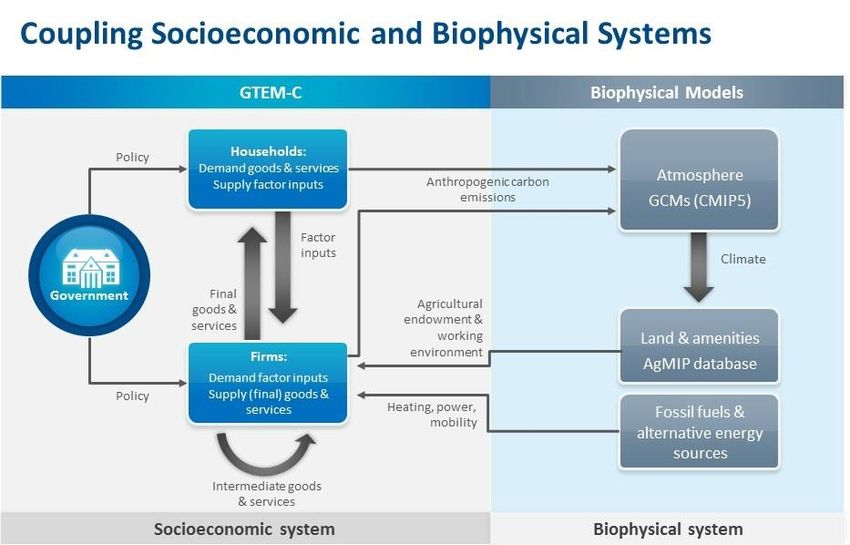
2 Methods

2.1 General modelling framework and past applications
The GTEM-C models was previously validated and used within the CSIRO’s Global Integrated
Assessment Modelling framework (GIAM) to study, for example, alternative GHG emissions
pathways for the Garnaut Review (Garnaut, 2011), the low pollution futures program (Australia,
2008) and the socio–economic scenarios of the Australian National Outlook (Hatfield-Dodds et al.,
2015). The GTEM-C model is a core component in the GIAM framework, a hybrid model that
combines the top-down macroeconomic representation of a computable general equilibrium
(CGE) model with the bottom-up details of energy production and GHG emissions. This model
builds upon the global trade and economic core of the Global Trade Analysis Project (GTAP)
(Hertel, 1997) database. Integrated modelling provides a unified framework to integrate
transdisciplinary knowledge about human societies and the biophysical world. This approach
offers a holistic understanding of the energy-carbon-environment nexus (Akhtar et al., 2013), and
has been intensively used for scenario analysis of the impact of possible climate futures on the
socio−ecological systems (Masui et al., 2011; Riahi et al., 2011).

2.2 Overview of the GTEM-C model
GTEM-C is a dynamic general equilibrium and economy-wide model capable of projecting
trajectories for globally-traded commodities, like agricultural products. A predecessor of GTEM-C,
called Global Trade and Environment Model (Pant, 2007), was used in Nelson et al. ( 2014) to
analyse economic consequences from climate change effects on agriculture. Natural resources,
land and labour are endogenous variables in GTEM-C. Labour moves freely across all domestic
sectors, but the aggregate supply grows according to demographic and labour force participation
assumptions and is constrained by the available working population, which is supplied
exogenously to the model based on the UN median population growth trajectory (United Nations,
2013).

In GTEM-C the world economy is divided into a set of autonomous regions. Each region has a
representative household, who determines the supply of labour, savings, and the consumption of
goods and services. In each of the region, local production is divided into multiple commodity
sectors/industries. The regions interact with each other through trade and capital flows, and
regional households consume both domestic and imported goods. In each period, the global
economy is in “equilibrium” between the producers’ and consumers’ profit/utility maximizing
behaviours across all regions, while it also evolves “dynamically” as demographics and resource
constraints change.

GTEM-C also features detailed accounting for global emissions and energy flows. Humans produce
greenhouse gases by burning fossil fuels to generate energy for industrial and residential use.
Agricultural activity and industrial processes also yield greenhouse gases (GHG) emissions. This
determines the environmental footprint of human activities, and the consequential (negative)
environmental feedbacks. Governments, thus have a role in neutralizing the feedbacks through
policy intervention, such as the imposition of Pigovian taxes and emission permits. The model

8 | Economic shifts in agricultural production and global trade from climate change

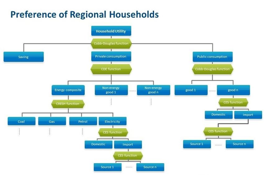
therefore offers a unified framework to analyse the energy-carbon-environment nexus. A
schematic diagram of GTEM-C is provided in Figure 1.

Figure 1. A schematic diagram of GTEM-C.

2.2.1 Household behaviours

GTEM-C assumes that there is a household representing the average behaviours of households in
each region. These representative households own and supply factor inputs of production, own
the regional income, and consume goods and services that are produced domestically and
imported. The households have a preference over the energy composite and other final goods
(Figure 2) that is represented by the Constant Difference in Elasticity (CDE) function (Hanoch,
1975). The households maximise utility given the prices and budget constraint. The CDE demand
system is calibrated to follow Engel’s law such that private demand for subsistent goods, such as
crops, livestock and processed food, will drop as regional income increases, whereas private
demand for luxury goods, such as manufacturing, energy and services, will rise as regional income
increases.

 Economic shifts in agricultural production and global trade from climate change | 9

Figure 2. Preference of the representative household.

2.2.2 Trade in GTEM-C

Both the households and industries consume goods and services that are produced domestically
and imported. Following GTAP, the GTEM-C model assume that the households and industries'
preference is represented by the Constant Elasticity of Substitution (CES) function, which allows
imperfect substitution between imported and domestic goods, and :
 
 −1 −1 −1
 = [ ( ) + ( ) ]

Equation 1

Here, is commonly known as the Armington elasticity of substitution between imported and
domestic goods, and and are the budget share parameters. For more details, please
see, for example, see Burfisher (2011) [p75]. Finally the imported good is, in turn, a CES
 
composite of shipments from various sources , , i.e.,

10 | Economic shifts in agricultural production and global trade from climate change

 
 −1 −1
 = 
 [∑ ( , ) ]
 
Equation 2

where is budget share parameter, and η is the elasticity of substitution among imports from
different sources. GTEM uses the same parameter values as in GTAP, which are econometrically
estimated and have been well tested in the literature.

2.2.3 Carbon emissions in GTEM-C

CO2 emissions in GTEM-C are calibrated to the RCP database: first a high emissions scenario,
where CO2 concentrations continue to increase resulting in an increase of radiative forcing
compared to pre-industrial levels of about 8 Wm-2 in 2100 (RCP8.5) (Friedlingstein et al., 2014) and
second, an active mitigation scenario, in which additional radiative forcing begins to stabilise at
about 4 Wm-2 after 2060 (RCP4.5) (Thomson et al., 2011). The RCP4.5 scenario limits global
temperature reaching 1.5˚ C, and the RCP8.5 scenario results in an increase in global temperatures
above 2˚ C by 2050. The ESMs used in the AgMIP study represents a wide cross section of climate
models from CMIP5, with a range of transient and equilibrium climate sensitivities between 1.3–
2.5 K and 2.44–4.67 K, respectively, consistent with the assessed likely range from all CMIP5
climate models of 1.1–2.5 K and 2.08–4.67 K, respectively. Climate projections from the ESMs are
used to force a set of Global Gridded Crop Models (GGCM) (Nelson et al., 2014). These GGCM
project crop yields at the global scale based on the different climate scenarios. These models were
systematically compared in the AgMIP and they take into account crop responses to atmospheric
CO2 concentrations as well as responses to water, temperature and nutrient stresses (Rosenzweig
et al., 2014). Agricultural productivity within GTEM-C was exogenously forced with projections
from the AgMIP database.

The current version of GTEM-C uses the Global Trade Analysis Project GTAP 9.1 database. We
disaggregate the world into 14 autonomous economic regions coupled by agricultural trade. Here,
we focus on the trade of four major crops: wheat, rice, coarse grains, and oilseeds (see all sectors
in Table 2) that constitute about 60% of the human caloric intake (Zhao et al., 2017). The RCP8.5
emission scenario was used to calibrate GTEM-C’s business as usual case, as current CO2 emissions
are tracking above RCP8.5 levels. A carbon price was endogenously calculated to force the model
to match the RCP4.5 emissions trajectory. This ensured internal consistency between emissions
scenarios and energy production. Climate change affects agricultural productivity, which leads to
variations in agricultural outputs. Given the global demand for agricultural commodities, the
market adjusts to balance the supply and demand for these commodities. This is achieved within
GTEM-C by internal variations in prices of agricultural products, which determine the position and
competitiveness of each region's agricultural sector within the global market, thus shaping the
patterns of global trade.

2.3 Scenario constructions
The results from the GTEM-C model are based on a reference scenario that follows RCP8.5 carbon
emissions and does not include perturbations in agricultural productivity due to climate. The
 Economic shifts in agricultural production and global trade from climate change | 11

agricultural productivities in the reference scenario are internally resolved within the GTEM-C
model to meet global demand for food assuming that technological improvements are able to
buffer the influence of climate on agricultural production. For the two counterfactual scenarios we
use future agricultural productivities obtained from AgMIP database to change GTEM-C’s total
factor productivities (hereafter agricultural shocks) of the four studied commodities. The
counterfactual scenario with no climate change mitigation follows the RCP8.5 emission
trajectories, same as the reference scenario, and includes exogenous agricultural shocks from the
AgMIP database. The scenario with climate change mitigation assumes an active CO2 mitigation by
imposing a global carbon tax, in which additional radiative forcing begins to stabilise at about 4
Wm-2 after 2060 (RCP4.5) following the CO2 emissions trajectory of the RCP4.5. The carbon
mitigation scenario includes exogenously perturbed agricultural productivities as per modelled by
the AgMIP project under RCP4.5.

All scenarios use 2008 as reference year and features 140 regions for all 57 GTAP commodities. As
mentioned before, we disaggregate the world into 14 regions: Brazil (BR); China (CN); East Asia
(EA); Europe (EU); India (IN); Latin America (LA); Middle East & North Africa (ME); North America
(NA, comprised by Mexico and Canada); Oceania (OC); Russia and neighbour countries (RU); South
Asia (SA); South East Asia (SE); Sub-Saharan Africa (SS) and United Stated (US) (Table 1); and 16
sectors (alphabetically ordered): coal, electricity, fisheries, foods, gas, industries, livestock, coarse
grains, oil, oilseeds, other crops, petroleum, rice, services, transport, and wheat (Table 2). The
aggregation was based on the regions’ significance to the global economy and agricultural trade as
well as their vulnerability to climate change. We note that alternative aggregations are possible,
and aggregations should be determined by the question under investigation.

In addition of investigating changes in the structure of the global agricultural trade network, we
also assess climate-related yield impacts and report subsequent changes in prices of key
commodities. The change is cost of these key commodities is reported as an aggregate for the
period 2050-2059. The results presented in Section 3.2 are based on a variable that reflects the
price of a commodity paid to producer (price). We found this variable is most affected by the
carbon mitigation policy. We calculated the percentage change difference in prices of the studied
commodities for the climate change scenarios, no climate change mitigation and climate change
mitigation, relative to the reference scenario.

Table 1. Regional aggregation.

 CODE NAME COUNTRY

 BR Brazil Brazil

 CH China China

 Hong Kong

 EA East Asia Japan

 Korea

 Mongolia

 Rest of East Asia

 Taiwan

 EU Europe Albania

 Austria

 Belarus

12 | Economic shifts in agricultural production and global trade from climate change

Belgium

 Bulgaria

 Croatia

 Cyprus

 Czech Republic

 Denmark

 Estonia

 Finland

 France

 Germany

 Greece

 Hungary

 Ireland

 Italy

 Latvia

 Lithuania

 Luxembourg

 Malta

 Netherlands

 Norway

 Poland

 Portugal

 Rest of Europe

 Romania

 Slovakia

 Slovenia

 Spain

 Sweden

 Switzerland

 United Kingdom

IN India India

LA Latin America Argentina

 Bolivia

 Caribbean

 Chile

 Colombia

 Costa Rica

 Ecuador

 El Salvador

 Economic shifts in agricultural production and global trade from climate change | 13

Guatemala

 Honduras

 Nicaragua

 Panama

 Paraguay

 Peru

 Rest of Central America

 Rest of South America

 Uruguay

 Venezuela

 MN Middle East and North Bharain
 Africa

 Egypt

 Iran Islamic Republic of

 Israel

 Kuwait

 Morocco

 Oman

 Qatar

 Rest of North Africa

 Rest of Western Asia

 Saudi Arabia

 Tunisia

 Turkey

 United Arab Emirates

 NA North America Canada

 Mexico

 Rest of North America

 OC Oceania Australia

 New Zealand

 Rest of Oceania

 RU Russia and neighbour Armenia
 countries

 Azerbaijan

 Georgia

 Kazakhstan

 Kyrgyztan

 Rest of Eastern Europe

 Rest of Europe

14 | Economic shifts in agricultural production and global trade from climate change

Rest of Former Soviet
 Union

 Russian Federation

 Ukraine

SE South East Asia Bangladesh

 Cambodia

 Indonesia

 Lao People's Democratic
 Republic

 Malaysia

 Philippines

 Rest of Southeast Asia

 Singapore

 Thailand

 Viet Nam

SA South Asia Nepal

 Pakistan

 Rest of South Asia

 Sri Lanka

SS Sub-Saharan Africa Botswana

 Cameroon

 Central Africa

 Cote d'Ivoire

 Ethiopia

 Ghana

 Kenya

 Madagascar

 Malawi

 Mauritius

 Mozambique

 Namibia

 Nigeria

 Rest of Eastern Africa

 Rest of South African
 Customs

 Rest of Western Africa

 Senegal

 South Africa

 South Central Africa

 Tanzania

 Economic shifts in agricultural production and global trade from climate change | 15

Uganda

 Zambia

 Zimbabwe

 US United States of United States of America
 America

Table 2. Sectoral mapping.

Marked with * the sector used in this study to calculate the structural index.

 Code Description

 Col Coal

 Ely Electricity

 Fish Fishing

 Forestry

 Foods Beverages and tobacco products

 Bovine meat products

 Dairy products

 Food products not elsewhere classified (nec).

 Meat products nec.

 Sugar

 Vegetable oils and fats

 Gas Gas

 Gas manufacture, distribution

 Industries Chemical, rubber, plastic products

 Construction

 Electronic equipment

 Ferrous metals

 Leather products

 Machinery and equipment nec.

 Manufactures nec.

 Metal products

 Metals nec.

 Mineral products nec.

 Minerals nec.

 Motor vehicles and parts

 Paper products, publishing

 Textiles

 Trade

 Transport equipment nec.

 Water

16 | Economic shifts in agricultural production and global trade from climate change

Wearing apparel

 Wood products

Livestock Animal products nec.

 Bovine cattle, sheep and goats, horses

 Raw milk

 Wool, silk-worm cocoons

Coarse grains* Cereal grains nec.

Oil Oil

Oilseeds* Oil seeds

Other crops Crops nec.

 Plant-based fibers

 Sugar cane, sugar beet

 Vegetables, fruit, nuts

P_C Petroleum, coal products

Rice* Paddy rice

 Processed rice

Services Business services nec.

 Communication

 Dwellings

 Financial services nec.

 Insurance

 Public Administration, Defense, Education, Health

 Recreational and other services

Transport Air transport

 Transport nec.

 Water transport

Wheat* Wheat

 Economic shifts in agricultural production and global trade from climate change | 17

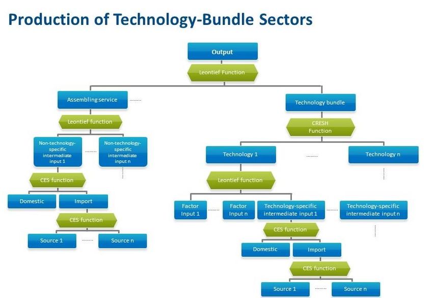
2.4 Overview of changes in agricultural productivity in GTEM-C
All economic activities related to agricultural production and consumption are recorded, as much
as the database allows. These activities include land use, employment, investment, inter-industrial
demand and end-user, as well as imports and exports. A detailed representation of the agricultural
supply chain allows GTEM-C to track the complex consequences of climate induced crop
productivity changes through different channels and in various causal directions.

Specifically, the production of an agricultural sector has a tiered structure (Figure 3). At the top
tier, industrial output is a Leontief function of a fuel-factor composite, and other intermediate
inputs. The fuel-factor composite is either a Leontief or a Constant Elasticity of Substitution (CES)
function of the fuel composite and the factor composite, allowing different levels of
substitutability between fuel and other inputs. The fuel composite is a CRESH function of coal,
petroleum products, gas, and electricity, while the factor composite is a CES function of natural
resources, land, labour and capital. Coal, gas, petroleum products, electricity and other
intermediate inputs are, again, CES aggregates of imported and domestic goods.

Figure 3. Schematic diagram of the technology-bundle sectors in GTEM-C.

We use the AgMIP (Elliott et al., 2015; Rosenzweig et al., 2014) dataset to perturb (hereafter ‘to
shock’) agricultural productivities in GTEM-C. The AgMIP database comprises simulations of
projected agricultural production based on a combination of physiologically driven global gridded
crop models (GGCM), earth system models (ESMs) and emission scenarios. Here we shock GTEM-C
agricultural production of four key commodities: coarse grains, oilseeds, rice and wheat, which
18 | Economic shifts in agricultural production and global trade from climate change

projections were obtained from seven AgMIP GGCMs accessed in January 2016
(https://mygeohub.org/resources/agmip): EPIC, GEPIC, pDSSAT, LPJml, LPJ-GUESS, IMAGE-LEITAP
and PEGASUS. The crop yield projections of the selected commodities are based on five ESMs:
HadGEM2-ES, IPSL-CM5A-LR, MIROC-ESM-CHEM, GFDL-ESM2M and NorESM1-M (see Table 1 in
Villoria et al., 2016). Our scenarios are based on two contrasting RCP trajectories, 4.5 and 8.5. The
very optimistic mitigation scenario that corresponds to RCP2.6 (van Vuuren et al., 2011) was not
included in our study for two reasons: first, the AgMIP database contains a limited number of
simulations for the four analysed commodities for RCP2.6 compare to RCPs 4.5 and 8.5. Second, it
would be necessary to include into GTEM-C a negative carbon emissions technology in order to
achieve the first Shared Socio-economic Pathway that corresponds to the RCP2.6’s CO2 emissions
trajectory.

2.5 An example of the influence of climate change on agricultural
 yields: maximum temperatures in the Australian winter cereal
 region
Recent studies have found that global agricultural production has declined in the last couple of
decades due to extreme weather events (Hochman et al., 2017; Lesk et al., 2016). Drought and
extreme heat are responsible for a decline of about 10% in the production of global cereals from
1964 to 2007 (Lesk et al., 2016). In Australia, for example, potential yield of wheat decreased by
27% since 1990 due to extreme weather caused by climate change (Hochman et al., 2017).
Potential yield is defined as the yield that can be achieved under current best management
practice with well-adapted commercial varieties and known technologies. About a third of the
annual variability in global agricultural yields is caused by climate variability (Howden et al., 2007)
and the interaction between climate variability and climate change threatens the sustainability of
traditional agricultural systems. Assuming that the area of cropped land cannot change
significantly in the future if biodiversity and conservation goals are to be met (Porfirio et al., 2016;
Watson et al., 2013); the other two mechanisms to cope with an increasing demand are
technological advancements (Hu and Xiong, 2014; Munns et al., 2012; Pallotta et al., 2014) and
agricultural trade.

Maximum temperatures during cereals flowering stage are crucial to determine crop yields. For
example, some of the consequences of heat stress on wheat flowering stage (during the months of
September and October in the Southern Hemisphere) are: premature leaf senescence, reduced
photosynthesis, reduced seed set, reduced duration of grain-fill, reduced grain size, and finally
reduced grain yield. We compiled data of maximum temperatures for September and October for
the winter cereal region in Australia (grey region in the map in Figure 4). The baseline period
shows average values of maximum temperature for 1951-1980. When we compared the baseline
maximum temperatures with more recent data, we see that the values for the 2000s are shifted to
the right, which means that maximum temperatures during these months are getting warmer than
the baseline (hatched lines in the middle plot in Figure 4). Future a projections of maximum
temperatures from the Australian Earth System Model, Access 1.3 (Bi et al., 2013), based on the
high carbon emissions Representative Concentration Pathway (RCP 8.5) are projected to be
warmer than today's averages. Globally, this is equivalent to an increase in temperatures above 2˚
C by 2050.

 Economic shifts in agricultural production and global trade from climate change | 19

Figure 4. September and October maximum temperatures for the Australian winter cereal region.

The baseline or historical periods corresponds to 1951-1980. The current periods corresponds to 2003-2013 (values
from the baseline period are hatched in grey), and the future periods to 2021-2050. The future projections of
maximum temperature are from the Australian Earth System Model, Access 1.3 (Bi et al., 2013), based on the high
carbon emissions Representative Concentration Pathway (RCP 8.5). This high carbon emissions scenario results in
an increase in global temperatures above 2˚ C by 2050.

20 | Economic shifts in agricultural production and global trade from climate change

2.6 Mathematical characterisation of the trade network
To quantify the structural changes in the agricultural trade network, we developed an index based
on the relationship between importing and exporting regions as captured in their covariance
matrix. We represent the spectrum of the eigenvalues of this covariance matrix as the elements, sij
of a diagonal NxN matrix. It is natural to interpret a rapidly converging spectrum as indicative of a
trade network dominated by just a few importers and exporters while a flat spectrum of
eigenvalues implies a network with many more equal actors. We capture this difference by using
Shannon’s entropy, a metric widely used in ecology, defining the structural trade index called S. A
smaller value of S represents a centralised network structure where export/import flows are
dominated by few regions, larger values of S suggest a more distributed trading structure where
export/import flows are more uniformly distributed between all regions. We tested if the S index
could capture historical shocks of the agricultural trade network. So we first applied our index on
bilateral trade data for the period 1870 to 2014 from the Correlates of War Project Data Set
version 4.0 (Barbieri and Keshk, 2012). Second we applied the metric to the agricultural global
trade data from the Food and Agricultural Organization (FAO) of the UN (FAOstat, 2016) for the
period 1986-2010 focusing on the four selected commodities. Third, we applied the metric to the
projections for the different GCMs and RCPs scenarios based on the GTEM-C model.

The S metric seeks a single number to quantify the relationship between importing and exporting
regions. The NN import-export matrix P encapsulates structural information about the global
trade network, here of N=14 regions. Each entry pij in P represents the value of exports from
region ri to region rj. Equally, each entry pji represents the value of imports by region rj from
region ri. Hence the i’th row of matrix P can be interpreted as an N-dimensional vector of regions
to which region i exports with the components of the vector equal to the quantity of exports
received from region ri. Conversely, column j of P can be interpreted as an N-dimensional vector of
regions from which region j imports with the components of the vector equal to the quantity of
imports received from region ri. If the trade network is regarded as a set of NN edges or links,
then the import-export matrix can be interpreted as the adjacency matrix of a directed graph with
edges weighted by the trade in each direction between pairs of regions. Conventionally, we
normalise the pij values by the total volume of trade so that,
 
∑ = 1
 −1

Equation 3

The resilience of the trade network to interruptions of supply by exporting countries or to inability
to pay by importing countries is related to its relational structure.

A direct measure of the structure of the network is provided by the Shannon entropy (Simpson,
1949) of the matrix P given by,
 
 = −∑ log 2 
 −1

Equation 4

 Economic shifts in agricultural production and global trade from climate change | 21

This measure has been proposed for applications in both human and natural sciences; see for
example, see Phillips and Conviser (1972) and Bonchev and Buck (2005). However it is easy to see
that H is unaffected by any permutation of the pij values so it cannot convey information about the
relational structure (from where to where) of the trade network, only about its general structure.

Here we propose a novel approach. The import\export matrix P can be reconstructed from a set of
simpler (rank 1) matrices Ei formed from the singular vectors and scaled by the singular values.

 = 

Equation 5

 = 1 + 2 + ⋯ 

Equation 6

 = 

Equation 7

Each column of Ek is a multiple of , the k’th row of U, the left singular vector and each row is a
multiple of , the transpose of the k’th column of V, the right singular vector. The component
matrices are orthogonal to each other in the sense that

E j EkT = 0, j ¹ k

Equation 8

The norm of each component matrix is just the singular value

 Ek = s k

Equation 9

So the size of the contribution each Ek makes to reproducing P is just the associated singular value.
This means that the singular values are the principal components.

From an information theoretic point of view, we are interested in how much information is
needed to reconstruct P to a given level of accuracy. If just the first few Ek are enough to
reproduce most of the P correctly because they are dominant, then the information content of the
network is small and its Shannon entropy, H will be small. If all the Ek are equally necessary, then

22 | Economic shifts in agricultural production and global trade from climate change

its information content is maximal and its H will be large. Hence an H formed from the spectrum of
sigmas produced by the singular value decomposition of P is all we need.

We define the information entropy of the trade network therefore as,
 
 = −∑ ̂ log 2 ̂ 
 =1

Equation 10

where ̂ are singular values of P.

S formed in this way will tend to large values when the import export network is well connected
with trade spread across all the regions. When the network simplifies and is dominated by a few
large exporters and importers, S will be small and the network will be more connected. Analysis
and plots were produced using R software (R Development Core Team, 2014).

 Economic shifts in agricultural production and global trade from climate change | 23

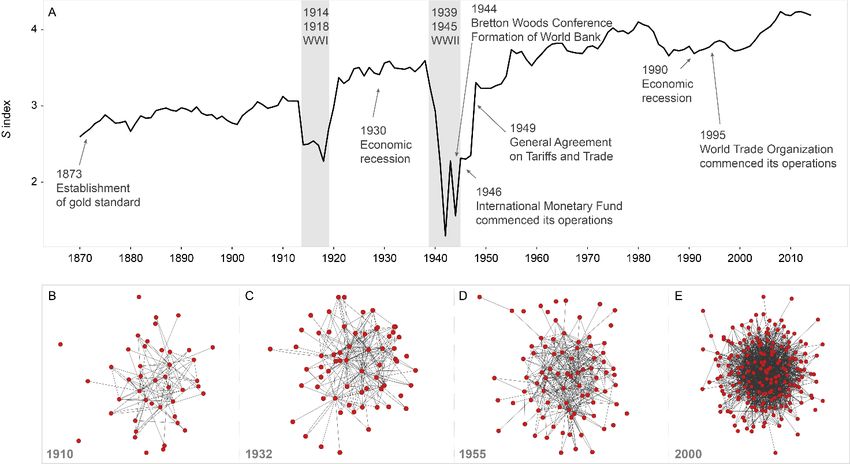
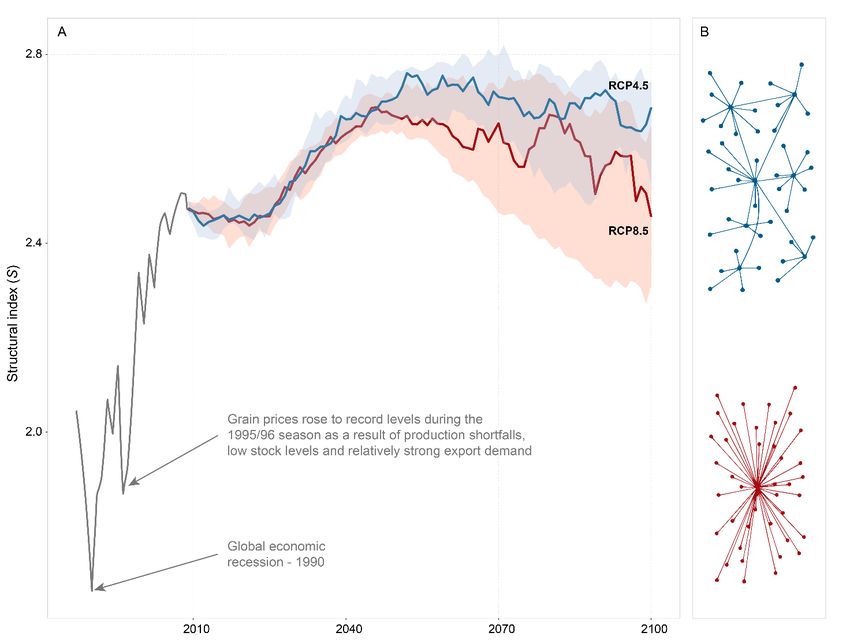
3 Results
3.1 Change in the global trade network
3.1.1 Testing the performance of the S structural metric

We tested the performance of the S index by using publicly available bilateral trade data from the
Correlates of War Project Data Set version 4.0 (Barbieri and Keshk, 2012). The bilateral trade
dataset (Barbieri et al., 2009) tracks total national trade and bilateral trade flows between states
from 1870-2014. Figure 5 shows a positive trend towards the end of the time series, indicating
that the structure of the global trade network becomes more decentralised and there are more
imports/exports interactions between the regions. It is important to mention the strong influence
of geopolitical and institutional events, such as the First and Second World Wars on the structure
of the global trade network. Each of these tragic events reduced the numbers of connections in
the global trade network, as it is captured by lower values of the S metric. Figure 5 highlights the
emergence of, for example, The International Monetary Fund (IMF) and the General Agreement of
Tariff and Trade (GATT), as corrective economic measures in the aftermaths of the Second World
War. Our results suggest that despite the economic recession in 1990, the structure of the global
trade network has been maintained.

Figure 5. Historical evolution of the structure of the global trade network for the period 1870-2014.

(A) We illustrate the historical evolution of the global trade network by using bilateral trade data from the
Correlates of War Project Data Set version 4.0 (Barbieri and Keshk, 2012). The bilateral trade dataset (Barbieri et al.,
2009) tracks total national trade and bilateral trade flows between states from 1870-2014. We developed a metric
called S based on Shannon’s entropy metric, which measures the structure of the trade network by quantifying the
underlying relationship between importing and exporting regions (Mathematical characterisation of the trade
network). Small values of the S index represent a centralised network structure, where export/import flows are
dominated by few regions, while larger values of S characterise a more decentralised trading structure, where

24 | Economic shifts in agricultural production and global trade from climate change

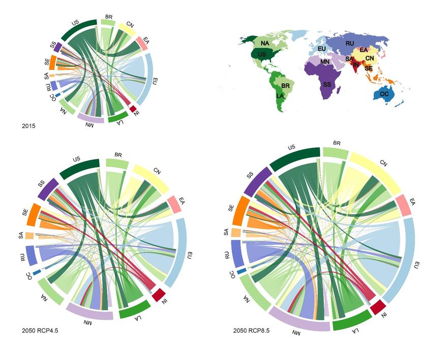
export/import flows are more uniformly distributed between all regions. (B) to (E) Network plots characterising the
structure of the global trading network from the beginning of the 20 th century to the beginning of the 21st century.

3.1.2 A visual characterisation of change in global trade

Aggregate patterns of global trade of the four studied commodities under RCP4.5 and RCP8.5 are
shown in Figure 6. The circular plots in Figure 6 are scaled according to the total global trade of the
analysed commodities in our model ensemble for the years 2015 and 2050. Our model estimates
that the value of global agricultural trade in USA billions of dollars (US$ 2007) was 144 US$ in
2015, this number is comparable with data from the United States Department of Agriculture that
reported a value of 136.7 US$ for 2015 (United States Department of Agriculture, 2015a, 2015b).

The structure of global agricultural trade projected to 2050 with and without the carbon
mitigation scenarios is significantly different from the current reality. These results suggest that
the total amount of trade is slightly bigger under the RCP8.5 scenario than in RCP4.5. The amount
of agricultural commodities imported by Sub-Saharan Africa will increase dramatically compared
to the baseline year (2015), this is because the largest increase in human population in the next
few decades will occur in this region, with a subsequent increase in the demand for food. When all
four commodities are aggregated, the differences in the patterns of trade in 2050 as shown in
Figure 6 are subtle. However, it is possible to see a significant increase in the amount of
commodities imported or exported to and from China, as the wedge that represents this region of
the world gets larger in RCP8.5 (Figure 6). In order to understand these subtleties, it is necessary
to analyse each commodity independently.

 Economic shifts in agricultural production and global trade from climate change | 25

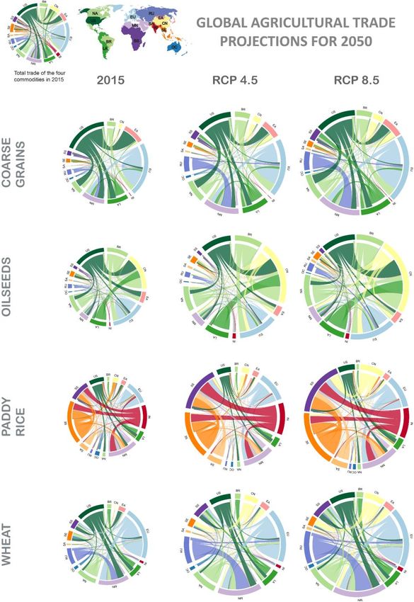
Figure 6. Total global trade of four aggregated commodities: coarse grains, oilseeds, rice and wheat, among 14
regions for the year 2050 under two RCP scenarios.

The links’ colours in the circular plots correspond to the exporting regions. The circles are scaled according to the
total global trade for the corresponding years. The base year (top left) shows total global trade in 2015. The RCP4.5
and RCP8.5 scenarios account for the effect of climate change on agricultural production and emission trajectories
for RCP4.5 and RCP8.5, respectively. The CSIRO version of the Global Trade and Environment Model (GTEM-C) was
used to project the full economy. Agricultural productivities within GTEM-C were exogenously forced with data
from the Agricultural Model Intercomparison and Improvement Project (AgMIP). The regions are: Brazil (BR); China
(CN); East Asia (EA); Europe (EU); India (IN); Latin America (LA); Middle East & North Africa (ME); North America
(NA); Oceania (OC); Russia and neighbour countries (RU); South Asia (SA); South East Asia (SE); Sub-Saharan Africa
(SS) and United Stated (US).

Figure 7 shows the global trading patterns for the years 2015 and 2050 for each commodity based
on the two carbon emissions scenarios. For example, the coarse grains market is dominated by US
and Europe and the projections to 2050 show small changes in the structure. For example, under
both scenarios, with and without carbon mitigation, the US is projected to shrink its exports to the
rest of the world, as Russia and neighbour regions, Brazil and China would increase coarse grains
exports. Patterns of global trade for oilseeds do not change dramatically by 2050.

The projections of trade for paddy rice for 2050 for the two carbon mitigation scenarios show a
significant increase in the demand in Sub-Saharan Africa, as population reaches 2200 million,
based on the UN Population Prospects (UN, 2017). However, the main difference between these
26 | Economic shifts in agricultural production and global trade from climate change

scenarios is that under RCP4.5 the major exporters to Sub-Saharan Africa would be India and
South-East Asia, whereas under RCP8.5 China would also become a major exporter of this
commodity (Figure 7).

The global trading patterns for wheat exports and imports show some changes in major wheat
exporters. This is related to the influence of climate on this particular crop. Relative to the baseline
year, 2015, wheat exports to Sub-Saharan Africa and Middle East and North Africa are projected to
increase significantly. Again, this is because the largest increase in human population in the next
few decades will occur in Africa. However, the baseline year shows that the major exporters to
these regions are US, Europe and North America (Table 1) (Figure 7). The projection based on the
carbon mitigation scenario shows that Russia and neighbour countries overtake US exports to
Middle East and North Africa, North America and Europe remain relatively constant, while under
RCP8.5 China’s wheat exports to Middle East and North Africa duplicate (Figure 7). Our simulations
generate a new link in the wheat trading pattern in 2050 from China to South East Asia. The
response of the global trade patterns to the different RCP emissions scenarios is uneven, reflecting
different regional impacts of climate change on agricultural production and the uneven effect of a
carbon price on regional economies, assuming no institutional changes.

 Economic shifts in agricultural production and global trade from climate change | 27

Figure 7. Global trade for the four studied commodities: coarse grains, oilseeds, rice and wheat, among 14 regions
for the year 2050 under two RCP scenarios.

The links’ colours in the circular plots correspond to the exporting regions. The circles are scaled according to the
total global trade for the corresponding years. The base year (top left) shows total global trade aggregated for the
four studied commodities in 2015. The RCP4.5 and RCP8.5 scenarios account for the effect of climate change on
agricultural production and emission trajectories for RCP 4.5 and RCP 8.5, respectively. The CISRO version of the
Global Trade and Environment Model (GTEM-C) was used to project the full economy. Agricultural productivities
within GTEM-C were exogenously forced with data from the Agricultural Model Intercomparison and Improvement
Project (AgMIP). The regions are: Brazil (BR); China (CN); East Asia (EA); Europe (EU); India (IN); Latin America (LA);
Middle East & North Africa (ME); North America (NA); Oceania (OC); Russia and neighbour countries (RU); South
Asia (SA); South East Asia (SE); Sub-Saharan Africa (SS) and United Stated (US).

28 | Economic shifts in agricultural production and global trade from climate change

3.1.3 A mathematical characterisation of change in global trade

Our projections based on GTEM-C suggest that there are changes in both the volume and patterns
of agricultural trade. We used the S index (see Section 2.6) to study changes in the agriculture
trade network, induced by climate impacts on agricultural. Small values of the S index represent a
centralised network structure, where export/import flows are dominated by few regions, while
larger values of the S index characterise a more decentralised trading structure, where
export/import flows are more uniformly distributed between all regions. The projected dynamics
of S for all model realisations and the ensembles are shown in Figure 8. We also tested the
performance of the index on a historical global agricultural trade dataset from the FAO (FAOstat,
2016) that accounts for the four studied crops, for the period 1986-2007. We observed two
significant drops in the value of the index in the historical period (grey line in Figure 8). The first
significant drop, i.e. the structure of the agricultural trade network becomes more centralised,
reflects the economic recession in the late 1980’s. The second drop in 1995-1996 relates to
climatically adverse conditions that resulted in agricultural production shortfalls. As a
consequence, grain prices rose to record levels (Food and Agriculture Organization of the United
Nations, 1996). The shortage in production and the rise in grain prices affected the structure of the
global agricultural trade network.

The evolution of the agricultural trade network from 2008 to 2100 (Figure 8) shows a period of
stability where the small differences in the climate responses of the RCP scenarios have little
impact on the structure of the trade network. Then a period of growth from about 2035–2060,
where under both scenarios global warming increases the amount of agricultural trade. And a
diverging phase, from about 2065–2100, where the global trading structure remains stable under
RCP4.5 while under RCP8.5 it becomes more centralised. As a consequence of climate change,
under RCP8.5 just a few regions will dominate export markets, while under RCP4.5 more regions
will be involved in global trade as either importers or exporters.

 Economic shifts in agricultural production and global trade from climate change | 29

Figure 8. Historical and projected changes in the global trading structure under the RCP4.5 and RCP8.5 climate
scenarios.

We present a structural index (A), based on Shannon’s entropy metric, that quantifies the underlying relationship
between importing and exporting regions. Smaller values of the structural index represent a simpler trading
network. Shown in grey, the historical trend of changed in the global trading network of the fours studied
commodities based on data from FAO database from 1986 to 2007. From 2008 onwards are projections of changes
in the global trade network based on outputs from the CSIRO version of the Global Trade and Environment Model
(GTEM-C). If the structural index increases, the trading network is becoming more distributed. If the structural index
becomes smaller, the network becomes more centralised. The projections revealed that under RCP8.5 (red) the
global trading structure becomes more centralised. While under RCP4.5 (blue) CO 2 mitigation scenario the global
trading structure becomes more distributed. (B) Network plots characterising the structure of the global trading
network from decentralised (top) to centralised (bottom).

3.2 Understanding the cost of mitigation versus the cost of
 adaptation

3.2.1 Variability of crop prices as modelled by GTEM-C

We explored the cost of transitioning to a low carbon economy while accounting for the impact of
future climates on crop yields and the demand for food of a growing human population. Figure 9
provides an overview of crop prices averaged for the period 2050-2059 as modelled by GTEM-C
under the carbon emissions scenarios based on RCP4.5 and RCP8.5, relative to the reference
scenario. Each box in Figure 9 contains information about price from our simulations, which
systematically combined GGCM, ESM and RCP scenarios in GTEM-C. The results suggest that there
is high variability in the response of agricultural production to climate change and impact on prices
30 | Economic shifts in agricultural production and global trade from climate change

(‘price’ reflects the price of a commodity paid to producer) under RCP8.5, showing a median value
for ‘price’ (black line in Figure 9) close to zero, i.e. not different from the prices calculated in the
references scenario for the period 2050-2059. However, the mean value in the RCP8.5 scenario is
about 11% increase in ‘price’ of the studied commodities (red dotted line in Figure 9). The results
for ‘price’ in the mitigation scenario, RCP4.5, are less variable, with exception of an outlier. The
median in the mitigation scenario is slightly above zero (black line in Figure 9)

Figure 9. Variability of crop prices as modelled by GTEM-C for aggregated commodities.

Here we show data for two contrasting climate change mitigation scenarios across crop aggregates (n = 4), global
gridded crop models (n=7), earth system models (n = 5), scenarios (n = 2), and regions (n = 14). The variable PRICE is
reported as percentage change for a climate change scenarios (RCP8.5, RCP4.5) relative to the reference scenario
(characterised by RCP8.5 carbon emissions and no changes in agricultural productivity) for the period 2050-2059.
The boxes represent first and third quartiles, and the whiskers show 5–95% intervals of results. The thick black line
represents the median, and the thin red dotted line, the mean value.

The variability in price within the results shown in Figure 9 relates to different agricultural
responses to climate change from the selected crops across the regions. Figure 10 shows the
distribution of the results for price per crop and scenario, for all GGCM, ESM and regions. All
commodities present higher averaged price values for the two scenarios in the period 2050-2059
relative to the reference scenario except for rice. Rice (RIC) shows small variability among the
simulations with a mean of -9.8% under RCP8.5 and -8.44% under RCP4.5. Wheat (WHT) shows
high variability under no carbon mitigation with a mean increase in prices of 23%, while under the
mitigation scenario the increase in prices reached 10.2%, this difference relates to a negative
effect of climate change on the regions this particular crop is grown. Coarse grains (CGR) show a
similar mean values under the two scenarios, of 20.4% for RCP8.5 and 18.5% for RCP4.5, with
slightly higher variability under the no mitigation scenario. Oil seeds (OSD) presents in average
higher prices under the mitigation scenario with an increase of 25.5% compared to a 10.2%
increase under the no mitigation scenario.

 Economic shifts in agricultural production and global trade from climate change | 31

Figure 10. Variability of crop prices as modelled by GTEM-C for all commodities.

Here we show data for two contrasting climate change mitigation scenarios across for key agricultural commodities.
RIC = Paddy rice; WHT = wheat; CGR = coarse grains and OSD = oilseeds. These results show aggregates of global
gridded crop models (n=7), earth system models (n = 5), scenarios (n = 2), and regions (n = 14). The variable PRICE is
reported as percentage change for a climate change scenarios (RCP8.5, RCP4.5) relative to the reference scenario
(characterised by RCP8.5 carbon emissions and no changes in agricultural productivity) for de period 2050-2059.
The boxes represent first and third quartiles, and the whiskers show 5–95% intervals of results. The thick black line
represents the median, and the thin red dotted line, the mean value (also printed under each box).

32 | Economic shifts in agricultural production and global trade from climate change