Beyond Forcing Scenarios: Predicting Climate Change through Response Operators in a Coupled General Circulation Model
←
→
Page content transcription
If your browser does not render page correctly, please read the page content below
Beyond Forcing Scenarios: Predicting Climate Change through Response
                                                                    Operators in a Coupled General Circulation Model

                                                                      Valerio Lembo1, , Valerio Lucarini1,2,3,a , Francesco Ragone4,
                                                                  [1] Meteorologisches Institut, Universität Hamburg, Hamburg, Germany
                                                             [2] Department of Mathematics and Statistics, University of Reading, Reading, UK
arXiv:1912.03996v2 [physics.ao-ph] 19 Apr 2020

                                                                              [3] Centre for the Mathematics of Planet Earth,
                                                                                  University of Reading, Reading, UK and
                                                                          [4] Laboratoire de Physique, ENS de Lyon, Lyon, France
                                                                                            (Dated: April 21, 2020)

                                                                                                   Abstract
                                                     Global Climate Models are key tools for predicting the future response of the climate system to a variety
                                                 of natural and anthropogenic forcings. Here we show how to use statistical mechanics to construct operators
                                                 able to flexibly predict climate change for a variety of climatic variables of interest. We perform our study on
                                                 a fully coupled model - MPI-ESM v.1.2 - and for the first time we prove the effectiveness of response theory
                                                 in predicting future climate response to CO2 increase on a vast range of temporal scales, from inter-annual to
                                                 centennial, and for very diverse climatic quantities. We investigate within a unified perspective the transient
                                                 climate response and the equilibrium climate sensitivity and assess the role of fast and slow processes. The
                                                 prediction of the ocean heat uptake highlights the very slow relaxation to a newly established steady state.
                                                 The change in the Atlantic Meridional Overturning Circulation (AMOC) and of the Antarctic Circumpolar
                                                 Current (ACC) is accurately predicted. The AMOC strength is initially reduced and then undergoes a slow
                                                 and partial recovery. The ACC strength initially increases due to changes in the wind stress, then undergoes
                                                 a slowdown, followed by a recovery leading to a overshoot with respect to the initial value. Finally, we are
                                                 able to predict accurately the temperature change in the Northern Atlantic.

                                                 a
                                                     v.lucarini@reading.ac.uk

                                                                                                      1
I.   INTRODUCTION

     Climate change is arguably one of the greatest contemporary societal challenges [1] and one
of the grand contemporary scientific endeavours [2]. The provision of new and efficient ways to
understand its mechanisms and predict its future development is one of the key goals of climate
science. Global climate models (GCMs) are currently the most advanced tools for studying future
climate change; their future projections are key ingredients of the reports of the Intergovernmental
Panel on Climate Change (IPCC) and are key for climate negotiations [3]. For IPCC-class GCMs,
future climate projections are usually constructed by defining a few climate forcing scenarios,
given by changes in the composition of the atmosphere and in the land use, each corresponding
to a different intensity and time modulation of the equivalent anthropogenic forcing. Typically,
for each scenario an ensemble of simulations is performed, with each member differing in terms
of initial conditions, applied forcing or chosen physical parametrizations. Subsequent phases of
the Coupled Model Intercomparison Project (CMIP, currently the sixth phase CMIP6 is active [4]),
which is part of the Program for Climate Model Diagnosis and Intercomparison (PCMDI), allowed
to define standardized experimental protocols for numerical simulations with several GCMs and
for the evaluation of the model runs [5, 6]. A bottleneck of this approach is that the consideration
of an additional forcing scenario requires running a new ensemble of simulations. Additionally,
for each forcing scenario, it is hard to disentangle the impact of each component of the forcing,
e.g. different greenhouse gases with their concentration pathways and land surface alterations in
geographically distinct regions. Finally, no rigorous prescription exists for translating the climate
change projections if one wants to consider different time modulations of a given forcing pathway,
e.g. a faster or slower CO2 increase.

     A.   Response theory and climate change

     A possible strategy to deliver flexible and accurate climate change projections is the construc-
tion of response operators able to transform inputs given by forcing scenarios into outputs in the
form of climate change signal. In this regard, it is tempting to use the fluctuation-dissipation theo-
rem (FDT) [7, 8], which provides a dictionary for translating the statistics of free fluctuations of a
system into its response to external forcings. The idea of using the FDT to predict climate change
from climate variability has been first proposed by Leith [9] and used by several authors thereafter

                                                 2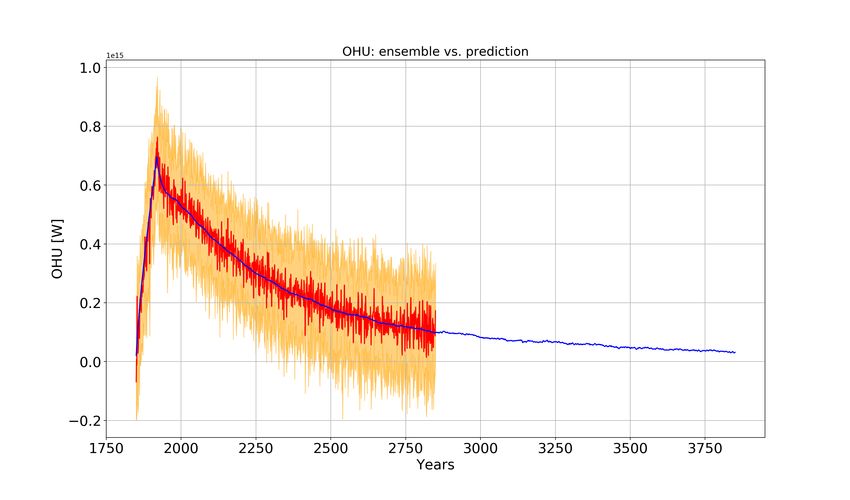
[10–12]. The FDT has recently been key to inspiring the theory of emergent constraints, which are
tools for reducing the uncertainties on climate change by looking at empirical relations between
climate response and variability of some given observables [13, 14].
   In the case of nonequilibrium systems, forced fluctuations contain features that are absent from
the free fluctuations of the unperturbed system [15]. Therefore, the applicability of the FDT for
such systems faces some serious theoretical and practical challenges [2, 16–18]. The climate is
a nonequilibrium system whose dynamics is primarily driven by the heterogeneous absorption of
solar radiation. The motions of the geophysical fluids with the associated transports of mass and
energy, as well as the exchanges of infrared radiation, tend to re-equilibrate the system and allow it
to reach a steady state [2, 19, 20]. Since the climate is not in equilibrium, climate change projects
only partially on the modes of climate variability, whilst climate surprises - unprecedented events -
are indeed possible when forcings are applied [17]. See Ghil and Lucarini [2] for a comprehensive
mathematical and physical discussion of the relationship between climate variability and climate
response to forcings.
   Response theory is a generalisation of the FDT that allows one to to predict how the statistical
properties of general systems - near or far from equilibrium, deterministic or stochastic - change
as a result of forcings. After the pioneering work by Kubo [7], response theory has been firmly
grounded in mathematical terms for stochastic [21] and deterministic [15, 22, 23] systems. The
use of response theory for predicting climate change has been successful in various numerical
investigations performed on models of various degrees of complexity, ranging from rather simple
ones [16], to intermediate complexity ones [12, 24, 25], up to simple yet Earth-like climate models
[18, 26]. The key step is the computation of the Green function for each observable of interest.
Then, the corresponding climate change signal is predicted by convolving the Green function with
the temporal pattern of forcing. Once the Green function is known, response theory allows one
to treat in a unified and comprehensive way forcings with any temporal modulation, ranging from
instantaneous to adiabatic changes.
   Note that, despite non-equilibrium conditions, a subtle relation exists between climate response
and climate variability. Indeed, natural modes of variability of the unperturbed system that can
be identified as prominent features in the autocorrelation or power spectra of climatic fields are
described by the Ruelle-Pollicott poles [2, 27, 28]. Such poles are responsible for extremely
amplified response of the system to a resonating forcing with suitably defined spatial and temporal
pattern.

                                                 3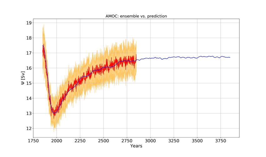
A similar heuristic approach, although not rooted in formal Ruelle’s [15, 22, 23] response the-
ory, was also proposed in the seminal work of Hasselmann [29], which raised some concerns
regarding its general applicability [30]. Despite this, recent attempts showed excellent skills for
a wide range of observables in GCM experiments [30]. The crucial point is that in these works
linear response formulas were applied to the output of individual experiments with GCMs. Ru-
elle’s response theory clarifies that the heuristic idea of Hasselmann [29] is instead mathematically
grounded if one considers ensemble averages rather than individual experiments.
   The climate models used so far to test response theory as formulated above [18, 26] lacked an
active and dynamic ocean, so that the multiscale nature of climate processes was only partially
represented. Capturing the slow oceanic processes is essential for a correct representation of the
multidecadal and long-time climatic response. Encouragingly, response theory has recently been
shown to have a great potential for predicting climate change in multi-model ensembles of CMIP5
atmosphere-ocean coupled GCMs outputs [31]. Blending together data coming from different
models is outside response theory theoretical framework, yet heuristically justifiable. However, a
proper treatment within the boundaries of the theory, based on ensemble of simulations with the
same model featuring an active ocean component, is still lacking.
   The response of a a slow (oceanic) climatic observable of interest has been investigated so far
in relation to the change in the dynamical properties of some other climatic observable , applying
a convolution product [32–35]. The strategy relies on constructing a linear regression between
the predictand and predictor using the properties of the natural variability of the system. While
indeed attractive and promising (and showing a good degree of success), this point of view cannot
be rigorously ported to climate change studies. Using the resulting transfer function to predict the
change of the observable of interest in a forced experiment would implicitly assume the validity
of the FDT; see discussion above.
   We remark that, in some cases (but not always), it is theoretically possible to use a climatic
observable for predicting the response of another climatic observable of interest in the presence
of an external forcing acting on the system. The possibility of using an observable as a surrogate
forcing able to retain predictive power depends of non-trivial properties of its frequency-dependent
response (its susceptibility, see below for a definition) and relies, in more practical terms, on the
possibility of separating two or more dynamically relevant time scales in the system [36]. See
recent applications of this idea in Zappa et al. [37] and, using a methodology based on adjoint
modelling, in Smith et al. [38].

                                                4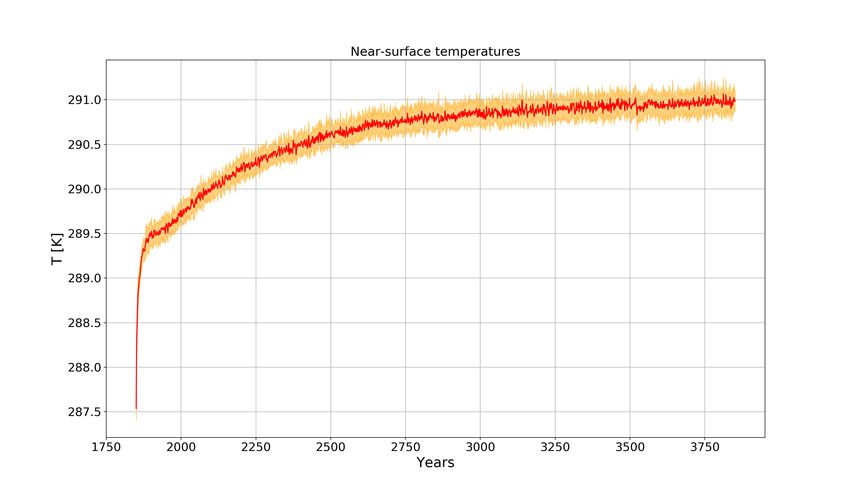
B.   Predicting Climate Change using the Ruelle Response Theory

      In this paper we show for the first time how the Ruelle’s response theory can be used to perform
successful centennial climate predictions in the fully coupled climate model MPI-ESM v.1.2 [39].
      We consider two ensemble experiments. One experiment features an instantaneous CO2 dou-
bling (2xCO2), and the outputs of its ensemble members are used to compute the Green functions
of several observables of interest, as described in the Methods section (Appendix A). We then
perform an ensemble of runs where the CO2 concentration is increased at the rate of 1% per year
until doubling (1pctCO2). We use the Green function computed with 2xCO2 to reconstruct the
response of 1pctCO2 and compare the prediction with direct numerical simulations.As discussed
in the Methods section, the Green function is defined for a period of 2000 years (y). Therefore, in
what follows we are able to perform predictions beyond the time frame simulated in the 1pctCO2
scenario (which is only 1000 y), thus showing very useful predictive power.
      First, we analyse the response of the globally averaged near-surface temperature (T2m ) on short
and long time scales. We then focus on two key aspects of the large-scale ocean circulation,
namely the Atlantic Meridional Overturning Circulation (AMOC) and the Antarctic Circumpolar
Current (ACC), and show that we can achieve excellent skill in predicting the the slow modes
of the climate response. We also look into the global ocean heat uptake (OHU) [40]. A non-
vanishing OHU indicates the presence of a global net energy imbalance. In current conditions, the
ocean is well-known [41] to absorb a large fraction of the Earth’s energy imbalance due to global
warming and to store it through its large thermal inertia, up to time scales defined by the deep
ocean circulation. Finally, we prove the validity of our approach for predicting the change in the
surface temperature in the North Atlantic, where the ocean deep water formation takes place. This
region features a complex interplay between radiative exchanges and meridional energy transport,
thus being particularly sensitive to the strength of the forcing and the changes in the large-scale
circulation.

II.    RESULTS

      A.   Global Mean Surface Temperature

      Figure 1 shows that the change of T2m under the 1pctCO2 scenario is predicted with very good
accuracy through response theory. The prediction is accurate both for the fast (first 70 y) and the

                                                  5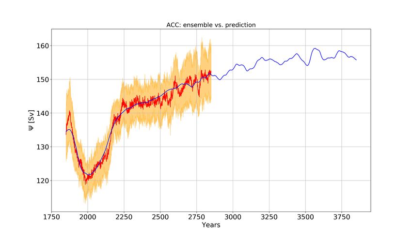
subsequent slow response. The time pattern of temperature change indicates that the contribution
of the fast feedbacks saturates after few decades, and the slow modes dominate the response for the
rest of the period. The warming goes on for multicentennial scales, in a way that is not captured
at all by models featuring a non-dynamic ocean [18, 26]. The importance of the slow modes
of climate response, associated with the oceanic thermal inertia, can be quantified considering
the ratio between the transient climate response (T CR) and the equilibrium climate sensitivity
(ECS); see Methods. Here we have T CR/ECS ≈ 0.5 (ECS ≈ 3.5K), which is much smaller
than what found (≈ 0.85) by Ragone et al. [26], indicating a very prominent role of the slow modes
of variability. The prediction obtained via response theory shows the establishment of steady state
conditions for times larger than 1000 y.
   The Green function - Fig. 5 - provides information on the time scales of the response. As a
result of the presence of slow oceanic time scales, the Green function significantly departs from a
simple exponential relaxation behavior, which is sometimes adopted to describe the relaxation of
the climate system to forcings [29, 42]. The idea of defining a general Green function as a sum of
multiple or infinite[28] exponential functions with different timescales, generalising Hasselmann’s
ideas - the so- called pulse-response method - and along the lines of previous studies [37, 43, 44]
is beyond the scope of our analysis and will be investigated further in a future work. In our case,
after a fast decrease for short time scales, the Green function tends to zero at a much slower pace
in for times longer than 100 y, in agreement with what reported by Held et al. [42].

   B.   Atlantic Meridional Overturning Circulation

   The AMOC is strongly influenced by buoyancy perturbations in the Atlantic basin [45]. It is
relevant at climatic level because it encompasses about 25% of the total (atmospheric+oceanic)
meridional heat transport [46]. The time series of annual mean AMOC strength in the 1pctCO2
scenario is shown in Fig. 2a. The AMOC strength undergoes a decrease by about 30%, reaching
its minimum in about 150 y. Successively, the AMOC slowly recovers.
   The prediction of the AMOC change obtained via response theory captures very well the en-
semble mean of the time evolution for the 1pctCO2 in the first 1000 y. The corresponding Green
function is shown in the inset of Fig. 6a. On short time scales, we have a reduction of AMOC, as a
result of the negative value of the Green function. On longer time scales (>100 y), a negative feed-
back acts as a a restoring mechanism, associated with a positive sign in the Green function. The

                                                6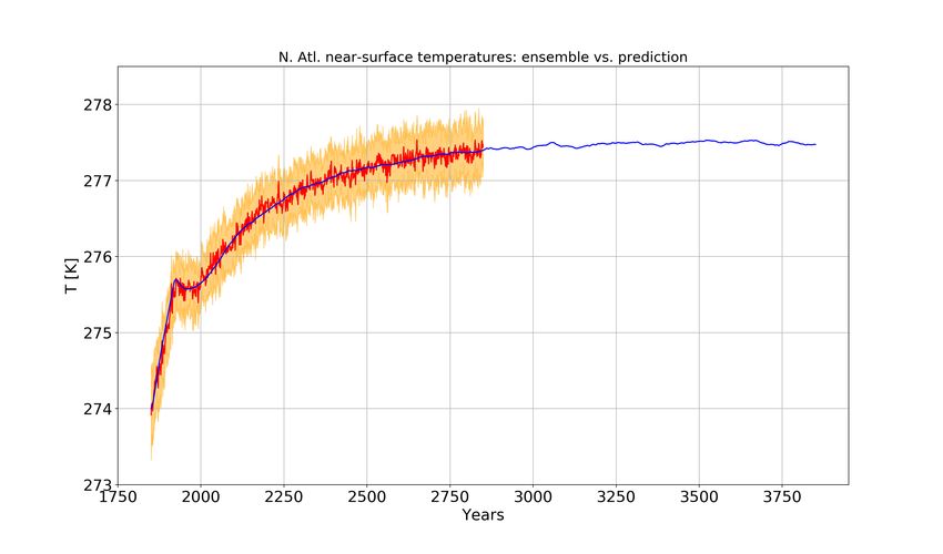
presence of fast (meaning here decadal) response associated with the GHG forcing has already
been found in other models [47, 48], and is most likely related to the timescales of the sea-ice
melting, consistently with paleoclimate simulations of the last interglacial climate with prescribed
freshwater influx from reconstructed sea-ice melting [49]. The slow recovery of the AMOC might
be understood as a heat [50–52] and freshwater [53] advection feedback.
   In the 1001-2000 y period, response theory shows that a steady state is progressively reached
over multi-centennial scales. The newly established AMOC is significantly weaker than the un-
perturbed AMOC, although a large ensemble spread is found. This is consistent with simulations
obtained from higher resolution versions of the same model [54], intermediate-complexity models
[48] and other fully coupled models inclusive of an interactive carbon cycle [55].

   C.   The Antarctic Circumpolar Current

   The ACC is by far the strongest large-scale oceanic current and its role in the general circulation
is two-fold. On one hand, it isolates Antarctica from the rest of the system, being associated with
a very strong zonal circulation in the Southern Ocean. On the other hand, although eminently
wind-driven, it marks the area of outcropping of deep water occurring at the southern flank of the
subtropical gyre, as part of the global-scale overturning circulation.
   The Green function is shown in the inset of Fig. 6b. We find that the initial strengthening of
the ACC can be associated with an increase in surface zonal wind stress (not shown here). Such a
surface forcing determines an enhanced Eulerian mean ACC transport, consistently with previous
low resolution simulations [56]. On decadal scales, we have a loss in the correlation between wind
stress and ACC, corresponding to the Green function turning negative after about 30 y. Beyond
these time scales, we have time-wise coherent response of the AMOC and ACC, underlying the
response of the global ocean circulation. Other models [57, 58] also feature such a behavior on
intermediate time scales, consistently with the idea that the two circulations are related via the
thermal wind balance [59].
   Figure 2b shows that the prediction of the ACC strength evolution in the 1pctCO2 scenario
is rather accurate for the first 1000 y, except for an underestimation of the positive short-term
response, which is smoothed out. This points to an insufficient ability of response theory in rep-
resenting the complex coupling between surface wind stress and downward momentum transfer.
Furthermore, we observe the presence of a strong variability (on decadal time scales) of the pre-

                                                7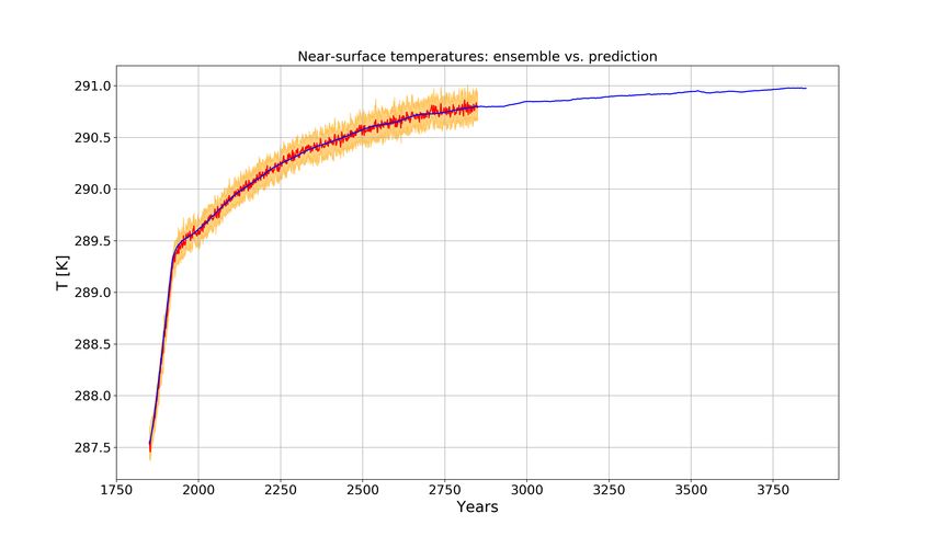
dicted signal. This might result from either the small ensemble size or, more interestingly, could
be the signature of the natural variability, encoded by a Ruelle-Pollicott pole [2, 27, 28]; see dis-
cussion in Sect. I A.
Note that in the 1001-2000 yrs period the ACC reaches an approximate steady state a bit later
than the AMOC, possibly as a result of having a larger inertia, consistently with the different
depth scales of the two currents [59, 60]. The AMOC maximum overturning depth scale is indeed
located at about 1 km, whereas the outcropping in the Southern Ocean is related to isopycnal
surfaces reaching much deeper. This has profound implications for setting the time scales of the
ACC and AMOC response. The propagation of deep water formation anomalies in the Northern
Hemisphere is in fact mediated by Kelvin waves in the Northern Atlantic, whereas much slower
interior adjustment through Rossby waves communicates the anomaly to the Southern Ocean [61].
D. Ocean heat uptake
Looking at the 2000 y of prediction in Fig. 3, we notice that response theory accurately predicts
the response at all time scales. The linearity of the OHU increase in the 70 y of integration comes
from the convolution of the singular component of the corresponding Green function with the
ramp, see the Methods section. After the CO2 concentration stabilizes, the OHU decreases towards
vanishing values. In the last 1000 y, response theory predicts a further decrease in the OHU down
to a value of the order of ≈ 5×10¹³ W . As the climate system as a whole relaxes towards the newly
established energetic steady state through the negative Planck feedback, each of its subcomponents
go through a process of relaxation. What we portray in Fig. 3 after year 1820 is the relaxation
of the slowest climatic component, namely the global ocean.. The remaining imbalance at the
end of the prediction can also be interpreted as either resulting from the ultra-long time scales
required for reaching rigorous steady state conditions, or as the signature of a model energy bias,
associated with non-vanishing energy budget at steady state, see discussion and Fig. 1 in Lucarini
and Ragone [62].
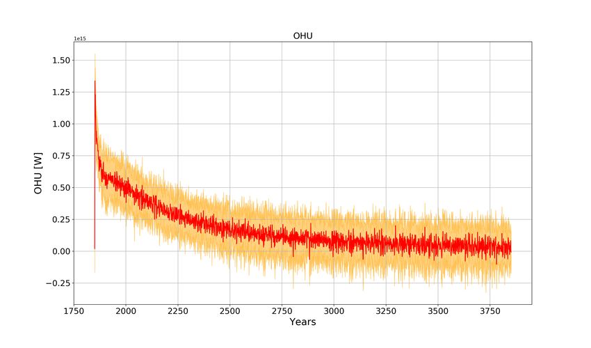
E. The North Atlantic cold blob
Finally, we study the surface temperature response for a domain covering the North Atlantic
(between 26◦ W and lon 53◦ W and latitude between 53◦ N and 69◦ N), thus including the areas
8where the deep water formation occurs. The region is identified as a peculiar spot for the effects
of the GHG forcing, since the sea-ice melting has been hypothesized to delay the surface warming
of this area compared to surrounding regions, through a weakening of the overturning circulation
[63]. Indeed - see Fig. 4 - the surface warming over the North Atlantic region is remarkably
different from the behavior of the rest of the extratropics, which features a time dependent response
(not shown here) similar in shape but somewhat amplified with respect to the global mean depicted
in Fig. 1. Indeed, a long-lasting plateau - a hiatus in the temperature increase of more than 100 y
- is observed around the end of the CO2 increase ramp in the North Atlantic. The plateau is well
captured by response theory, and comes in agreement with the AMOC weakening [63] predicted
in Fig. 2a. This result is non-trivial, given that such local response results from an interplay of
local factors and, as mentioned, the response of the large-scale oceanic circulation. This hints at
the potential of using response theory to identify global quantities that can be used as predictors
for the response of local observables [28].
III. DISCUSSION AND CONCLUSIONS
We have shown here that response theory is a valuable tool for predicting crucial aspects of
the response in the climate system to a prescribed forcing. All relies on obtaining the observable-
dependent Green function from model simulations. The Green function allows one to deal with
a continuum of time-dependent forcings, beyond the standard use of reference scenarios. Our
findings provide guidance to the climate modellers’ community on how to set up climate change
experimental protocols, minimising the need for computational resources. This is especially rele-
vant when one wants to study the overall impact and individual effects of multiple climatic forcings
or investigate geoengineering options.
We have made here use of a fully coupled climate model, highlighting the slow components
of the response associated with the oceanic modes of variability. The presence of a vast range of
active time scales in the system makes the prediction of the response theoretically challenging and
practically extremely relevant. Compared with previous contributions to the literature that have
attempted with a good degree of success the prediction of changes in slow climatic fields using
some form of linear regression, our approach is mathematically more robust as it derives directly
from basic results in non-equilibrium statistical mechanics.
We stress that response formulas based on Ruelle’s theory are rigorously valid, but only when
9considering ensemble averages. On one side, this clarifies the limits of validity of previous at-
tempts to apply similar formulas to individual model runs. On the other side, it indicates the
importance to consider large ensemble strategies when planning major computational efforts for
climate change projections.
The predicted changes in the AMOC and ACC feature clearly distinguishable fast and slow
regimes of response. The former is essentially different in the two branches of the global ocean
circulation, being the ACC subject to the effect of surface wind stress anomalies (substantially
underestimated, compared to actual simulations). The latter is found to be well correlated between
AMOC and ACC, as a signature of the forced response of the global ocean circulation circulation,
which they are both part of. Coherently with previous findings [59, 60], the ACC reaches a steady
state much later than the AMOC. The plateau in near-surface warming over the North Atlantic is
also related to the initial slowdown of the AMOC, and contrasts with the regular increase of the
surface temperature we find globally (and predict accurately).
We remark that the time-dependent transient and long-term evolutions resulting from the CO2
increase are qualitatively different for the various climatic observables investigated here. Nonethe-
less, in all considered cases response theory successfully predicts the time-dependent change.
Ruelle’s response theory provides a relatively simple yet robust and powerful set of diagnos-
tic and prognostic tools to study the response of climatic observables to external forcings. The
availability of a large number of ensemble members allows for constructing more accurate Green
functions and for studying effectively the response of a broader class of climatic observables. The
approach proposed here could be extremely useful to inform the planning of major computational
efforts for climate projections, putting such endeavours on firm theoretical grounds and optimizing
the use of computational resources.
We have dealt here with a forcing due only to changes in the CO2 concentration. This means
that the pattern of the forcing is determined by heating rate associated with a spatially homoge-
neous CO2 mixing rate. Within the linear regime, different sources of forcings can be treated
independently. The next step is to investigate other nontrivial forcings (e.g. aerosol forcings,
land-use change, land glaciers location and extension). As an example, response theory has been
proposed as a tool for framing geoengineering strategies and understanding its limitations [64].
Response theory provides a powerful formalism to tackle different problems related to the con-
cepts of feedback and sensitivity. A promising application is the definition of functional relations
between the response of different observables of a system to forcings, in the spirit of recent ap-
10plications (see, e.g. Zappa et al. [37]). This would allow to treat comprehensively the concept of
feedback across different time scales and define causal links between variables [28]. On a different
line, one of the most promising future applications will be given by the synergy between the for-
malism of response theory and the recently proposed theory of emergent constraints [13, 65]. The
combination of the two approaches could lead to much needed insights on the climate response to
forcings.
Additionally, along the lines of the pulse-response approach, it is in principle possible to try to
extract the characteristic time scales of the response of the system by fitting the Green functions
of the considered observables as a weighted sum of (in principle, infinitely many) exponential
functions. As explained in Refs. [28, 66], the time scales of the exponential functions are the
same for all observables. Instead, the weight of each exponential contribution does depend on the
observable of interest, with the response of rapidly equilibrating observables being dominated by
the fast time scales, while the opposite holds for observables associated with the slow components
of the system. The optimal fit can be obtained through a global optimisation procedure, where the
response of various different observables is simultaneously fitted to a sum of exponentials. We
will delve into this interesting problem of inverse modelling in a separate publication.
Clearly, in some applications one may want to test accurately to what extent nonlinear effects
are relevant, as the theory is also applicable to higher orders [16]. Some insights into the non linear
component of the response could also be obtained by appropriately combining forcings differing
in sign and magnitude [16, 17, 64]. Nonetheless, being based on a perturbative approach, response
theory (linear and nonlinear) has, by definition, only a limited range of applicability (e.g. one
cannot use it to treat arbitrarily strong forcings). Still, the non-applicability of response theory has
itself fundamental implications for the knowledge of the dynamics of the system one is studying.
At a tipping point [67–70] (or critical transition) the negative feedbacks of a system are overcome
by the positive ones and any linear Green function diverges as a result of the increase in the time
correlations of the system due to a critical Ruelle-Pollicott pole [2, 27], signalling the crisis of the
chaotic attractor [66]. Instead, near a critical transition, response operators do not converge unless
one considers very weak forcings [27, 36]. The experimental design provided here is thus also a
clear and mathematically sound strategy for the study of conditions leading to tipping points and
their role for the climate response [2, 69] in state-of-the-art climate models.
11Appendix A: Methods
1. Simulations
The analysis is based on two ensembles of simulations with Max Planck Institute Earth Sys-
tem Model (MPI-ESM) v.1.2 [39], using its coarse resolution (CR) version. It features, for the
atmospheric module ECHAM6 [71], of T31 spectral resolution (amounting to 96 gridpoints in
longitude and 48 in latitude) and 31 vertical levels, for the oceanic module MPI-OM [72] of a
curvilinear orthogonal bipolar grid (GR30) (122 longitudinal and 101 latitudinal gridpoints) with
40 vertical levels. The two ensembles, each including 20 runs, are based on two different sce-
narios. The first one features an instantaneous doubling in CO2 concentrations (from a reference
value of 280 ppm, characteristic of pre-industrial conditions) at the beginning of the simulations
(2xCO2), the other one an increase in the CO2 concentration at the constant rate of by 1% per
year, until the 2xCO2 level is reached after about 70 years; afterwards, the CO2 concentration is
kept constant (1pctCO2). The procedure for the construction of the ensemble is analogous to the
protocol for CMIP5 [73] and Grand Ensemble [74] experiments. A control run is performed for
2000 y with pre-industrial conditions. Each of the ensemble members is initialized from a state
of the control run. The initial conditions are sampled from the control run every 100 y, in order
to ensure sufficient decorrelation among the respective oceanic states (at least in the mixed layer
[75, 76]). The 2xCO2 simulations are run for 2000 y, while the 1pctCO2 simulations are run for
1000 y with the same 20 initial conditions. As an additional check, one of the 2xCO2 members is
prolonged for 2000 additional y, in order to investigate whether the model converges to the steady
state or there is an intrinsic model drift [77].
2. Retrieval of AMOC and ACC
Typically, the large-scale circulation in the ocean is measured in terms of the mass transport
across a suitably chosen section of a basin. The strength of the AMOC is computed as the verti-
cally integrated mass weighted meridional mass streamfunction across the latitude 26.5◦ N [78].
This is a standard diagnostics of the MPI-ESM model. The ensemble average of the AMOC vol-
ume transport amounts to 17.3 Sv, which is consistent with recent available measurements from
the RAPID monitoring array [79]. The ACC is roughly zonally symmetric, and its location is
closely related to the isopycnal slopes in the Southern Ocean. Traditionally[57], it has been mea-
12sured in terms of the strength of the mass transport across the Drake passage. Similarly, we take
the vertically integrated barotropic streamfunction difference between the 2◦ × 2◦ boxes centered
around the 68◦ W, 54◦ S and 60◦ W, 65◦ S locations. The ensemble average of the ACC is 138 Sv,
which is consistent with the multi-model mean estimate found in Mejers et al. [57], amounting to
155±51 Sv. It is also not far from the value commonly used as benchmark for the assessment of
climate models (173 Sv [80]).
3. Linear response theory
Response theories allow one to predict how the statistical properties of a system changes as
a result of acting modulations in its external or internal parameters. The validity of the corre-
sponding response formulas is heavily dependent on the hypothesis that the unperturbed system
is structurally stable, i.e., roughly speaking, far from bifurcations, or, in terms of geophysical sys-
tems, from tipping points (see related discussions in a climate context [18, 25–27]). Rigorous
derivations of response theories have been provided for the case of deterministic [15, 22, 23] and
stochastic [21] dynamics. We only remark here that statistical mechanical arguments encoded by
the chaotic hypothesis [81] (a non-equilibrium analogue of the ergodic hypothesis) indicate the
feasibility of the methodology proposed here.
In this paper we follow to a large extent the approach presented in [18] and [26] (see also
[16, 25]) for the study of a large ensemble of intermediate-complexity atmospheric model runs
and follow the deterministic route for response theory [15, 22, 23]. Let us consider a dynamical
system described by the state vector x , whose dynamics is described by the set of differential
equations ẋ = F (x ). We add a perturbation vector field of the form Ψ (x , t) = X (x )f (t), where
X is the structure of the forcing in the phase space and f its time modulation. The expectation
value of any observable Φ = Φ(x) can be written as:
∞
X (n)
hΦf (t)i = hΦi0 + hΦif (t) (A1)
n=1
(n)
where Φ0 is the expectation value in the unperturbed state, and the term Φf (t) gives the nth order
(1)
perturbative contribution. We consider here only the first order contribution hΦif (t). The linear
correction is given by the convolution of the linear Green function with the time modulation of the
perturbation: Z
(1) (1)
hΦif (t) = dσ1 GΦ (σ1 )f (t − σ1 ) (A2)
13(1)
where GΦ is the linear Green function of the generic observable Φ. For ease of notation we
have not indicated in equation A1 the dependence of the response on X, as in the applications
considered in this paper X is fixed and only the time modulation f is varied. Note that for a time
modulation f such that limt→0 f (t) = f0 , |f0 | finite, and f (t) = 0 if t < 0, as in the case of
f (t) = cH(t), where c is a nonvanishing constant and H is the Heaviside distribution (H(t) = 0
1)
for t ≤ 0 and H(t) = 1 for t > 0), one typically has that hΦif (0) = 0, as observed in this paper
for all observables except the OHU. In this latter case, one has limt→0 hΦif (t) 6= 0 because the
Green function has a singularity (in the form of a Dirac’s δ contribution) for t = 0 [28].
We remark that in previous works [32–35, 37], the linear prediction of the desired climate
observable is instead obtained by convolving time pattern of another climatic observable - the
driver - rather than the actual external forcing - with an effective transfer function - rather than
the true Green function. The conditions under which climate observables can be used as both
predictands and predictors have been discussed by Lucarini [28].
(1)
By taking the Fourier transform of the Green function GΦ , one obtains the linear susceptibil-
(1)
ity of the observable χΦ (ω), where ω is the frequency. The susceptibility gives the frequency
(1) (1)
response to a forcing f (t) as Φ̃ (ω) = χ (ω)f˜(ω), where with ˜· we indicate the Fourier trans-
f Φ
form. The susceptibility gives a spectroscopic description of the properties of the response of the
observable, and its analysis can give interesting information on the most relevant time scales and
related processes that determine the response of the observable.
4. Procedure for the retrieval of the Green functions
The strategy for testing the prediction of the mentioned key variables with the coupled model
ensembles is as follows. First, we compute the Green function from the 2xCO2 experiment. The
time variable is defined in such a way that the instantaneous doubling occurs at t = 0. Hence,
the time modulation of the forcing is given in this case by f (t) = f2xCO2 H(t), where H(t) is the
Heaviside function, and f2xCO2 is a constant depending on the amplitude of the forcing. Since the
radiative forcing is approximately proportional to the logarithm of the CO2 concentration, such a
constant is given by f2xCO2 = log(2) (it would be f2xCO2 = log(p) if the final CO2 concentration
were p times as large as the initial one). Equation A2 can be thus rewritten as:
d (1) (1)
Φ (t) = f2xCO2 GΦ (t) (A3)
dt f2CO2
14The outputs of the 2xCO2 experiments and the corresponding Green functions for the observables
described above are presented in Figs. 5-8.
In particular, the time evolution of OHU for this scenario is shown in Fig. 7. The positive
forcing due to the instantaneous CO2 doubling leads to an instantaneous jump in the OHU, leading
to an annual average value of more than 1 PW in the first year. Equation A3 then suggests that the
(1)
Green function GOHU has a singular behaviour at t = 0 (cfr. [28]), while a regular behaviour is
found for t > 0, corresponding to the negative radiative Planck feedback.
For all observables, we then use the Green functions above to perform predictions for the
1pctCO2 scenario using Eq. A2. Thanks to the proportionality of the radiative forcing to the
logarithm of the CO2 concentration, the time modulation of such forcing can be expressed as
f = f1pctCO2 r(t), where r(t) is a ramp function (cfr. Lucarini et al. [18] and Ragone et al. [26]):
0 tτ
where the time scale τ ≈ 70 y denotes the time needed to reach the doubling in the CO2 con-
centration and where f1pctCO2 = f2xCO2 because at the end of the ramp the CO2 concentration is
doubled.
From the Green function, one could in principle compute the susceptibility and perform a
spectral analysis of the properties of the response. However, the correct identification of spectral
peaks in the susceptibility requires a much richer statistics than what we have available here. The
reason is that, while the Green function is an integral kernel whose specific values at each t are
not of crucial importance per se, as it is their integrated contribution that determines the response,
in the case of the susceptibility it is extremely important to make sure that the signal to noise ratio
is very large at each individual value of ω. This translates into the fact that, despite the Green
function and the susceptibility being strictly connected, to obtain a satisfactory estimate for the
latter require a statistics orders of magnitude larger than for the former, and possibly different
and dedicated numerical estimation approaches [16, 17, 25]. An analysis of the susceptibility in
experiments similar to what done in this work was attempted in Ragone et al. [26], but using
ten times more ensemble members. We therefore do not present an analysis of the susceptibility.
While the analysis of the detailed frequency response of a climate model remains a very interesting
and promising topic, it has to likely wait until experiments with at least several hundreds ensemble
members will be available.
155. Equilibrium Climate Response and Transient Climate Sensitivity
Response theory allows to place on solid formal ground operational definitions of the sensitivity
of the climate system [2, 18, 26]. One of the most important indicators of the global properties of
the response of the system to climate change is the equilibrium climate sensitivity (ECS), which is
the long term (t → ∞) response of the observable T2m to an abrupt doubling of CO2 concentration
[3]. Another common measure of the response is the transient climate response (TCR), which is
the change in T2m realised in the 1pctCO2 scenario of at the end of ramp of the CO2 increase [82].
Using the formalism discussed in this paper, the ECS can be straightforwardly linked to the
(1)
susceptibility, because ECS = f2xCO2 χT2m (0) [2, 18, 26]. Additionally, the TCR can be computed
as the result at time t = τ of the convolution of the Green function of T2m with the forcing given
in Eq. A4. Indeed, more generally, the susceptibility can be interpreted as a generalised sensitivity
function. In particular, as explained in Ragone et al. [26], one can find an explicit functional
relation relation between TCR and ECS (sometimes referred to as realised warming fraction [3]):
+∞ (1)
1 + sinc(ωτ /2)e−iωτ /2 χT2m (ω)
Z
T CR
=1− (1)
dω (A5)
ECS −∞ 2πiω χT (0)
2m
where sinc(x) = sin(x)/x. The integrand in the second term on the right hand side of Eq.
A5 gives the contribution of each time scale to the inertia of the system. Note that this approach
allows for treating seamlessly the case of transient response to steeper or gentler increases of
CO2 . However, a detailed analysis of the relationship between TCR and ECS requires an accurate
estimate of the susceptibility, that as explained above is beyond the scope of this work.
The theory of emergent constraint has been used to study the ECS [83] and the TCR [84] in
climate models. The relationship between ECS and TCR proposed in Eq. A5 might be helpful
elucidating and better understanding such results.
16ACKNOWLEDGMENTS
Valerio Lembo was supported by the Collaborative Research Centre TRR181 ”Energy Trans-
fers in Atmosphere and Ocean” funded by the Deutsche Forschungsgemeinschaft (DFG, Ger-
man Research Foundation), project No. 274762653. Valerio Lucarini was partially supported by
the SFB/Transregio TRR181 project and by the Horizon2020 projects CRESCENDO (Grant no.
641816) Blue-Action (Grant No. 727852) and TiPES (Grant No. 820970). Simulations were per-
formed with Mistral, the Deutsches Kilmarechenzentrum (DKRZ) High Performance Computing
system for Earth system research (HLRE-3) supercomputer, projects No. um0005 and bu1085.
Author Contributions Statement
V. Le. ran the ensemble of simulations, performed the retrieval of the Green functions that
were used for the predictions and analysed the results. V. Lu. proposed and directed the work and
commented on the results. F. R. supported the numerical implementation of the response operators
and commented on the results. All authors equally contributed to the writing of the paper.
17Figure 1. Comparison between the simulated T2m in the 1pctCO2 scenario (thick red line with ensemble
mean uncertainty) and the prediction performed using the linear Green function in Fig. 5 (thick blue).
18(a)
(b)
Figure 2. Same as Fig. 1, for (a) AMOC at 26N (in Sv) and (b) ACC (in Sv). The predictions are performed
using the linear Green functions shown in Fig. 6.
19Figure 3. Same as Fig. 1 for the OHU (in W ). The prediction is performed using the linear Green function
shown in Fig. 7.
20Figure 4. Same as Fig. 1 for the surface temperature in the North Atlantic (in K). The prediction is per-
formed using the linear Green function shown in Fig. 8.
21Figure 5. Time series evolution of global mean T2m (in K) for 2xCO2 . The thick line the annually averaged
ensemble mean, the shaded areas denote the 1σ ensemble range. The inset shows the first 1000 y of the
linear Green function for global mean T2m (in Kyr−1 ), computed from the ensemble mean of the 2xCO2
experiment.
22(a)
(b)
Figure 6. Same as in Fig. 5, for (a) AMOC at 26N (in Sv) and (b) the ACC through the Drake passage (in
Sv). The linear Green functions are in Sv yr−1 ).
23Figure 7. Same as in Fig. 5, for OHU (in W). The linear Green function is in W yr−1 ).
Figure 8. Same as in Fig. 5, for the near-surface temperatures averaged in the North Atlantic region (in K).
The linear Green function is in K yr−1 ).
24[1] Tim Palmer and Bjorn Stevens. The scientific challenge of understanding and estimating climate
change. Proceedings of the National Academy of Sciences, 116(49):24390–24395, 2019.
[2] Michael Ghil and Valerio Lucarini. The Physics of Climate Variability and Climate Change. arXiv
e-prints, page arXiv:1910.00583, October 2019.
[3] Intergovernmental Panel on Climate Change. Climate Change 2013: The Physical Science Basis.
Press, Cambridge University, Cambridge Mass., 2013.
[4] V. Eyring, S. Bony, G. A. Meehl, C. A. Senior, B. Stevens, R. J. Stouffer, and K. E. Taylor. Overview of
the Coupled Model Intercomparison Project Phase 6 (CMIP6) experimental design and organization.
Geoscientific Model Development, 9(5):1937–1958, 2016.
[5] V. Eyring, M. Righi, A. Lauer, M. Evaldsson, S. Wenzel, C. Jones, A. Anav, O. Andrews, I. Cionni,
E. L. Davin, C. Deser, C. Ehbrecht, P. Friedlingstein, P. Gleckler, K.-D. Gottschaldt, S. Hagemann,
M. Juckes, S. Kindermann, J. Krasting, D. Kunert, R. Levine, A. Loew, J. Mäkelä, G. Martin, E. Ma-
son, A. S. Phillips, S. Read, C. Rio, R. Roehrig, D. Senftleben, A. Sterl, L. H. van Ulft, J. Walton,
S. Wang, and K. D. Williams. ESMValTool (v1.0) – a community diagnostic and performance met-
rics tool for routine evaluation of Earth system models in CMIP. Geoscientific Model Development,
9(5):1747–1802, 2016.
[6] V. Lembo, F. Lunkeit, and V. Lucarini. Thediato (v1.0) – a new diagnostic tool for water, energy and
entropy budgets in climate models. Geoscientific Model Development, 12(8):3805–3834, 2019.
[7] Ryogo Kubo. Statistical’Mechanical Theory of Irreversible Processes. I. General Theory and Sim-
ple Applications to Magnetic and Conduction Problems. Journal of the Physical Society of Japan,
12(6):570–586, 1957.
[8] U. Marini Bettolo Marconi, A. Puglisi, L. Rondoni, and A. Vulpiani. Fluctuation-dissipation: Re-
sponse theory in statistical physics. Phys. Rep., 461:111, 2008.
[9] C. E. Leith. Climate response and fluctuation dissipation. Journal of the Atmospheric Sciences,
32(10):2022–2026, 1975.
[10] V. A. Alexeev. Sensitivity to CO2 doubling of an atmospheric GCM coupled to an oceanic mixed
layer: A linear analysis. Climate Dynamics, 20(7-8):775–787, 2003.
[11] I. Cionni, G. Visconti, and F. Sassi. Fluctuation dissipation theorem in a general circulation model.
Geophysical Research Letters, 31(9):L09206, 2004.
25[12] Andrey Gritsun and Grant Branstator. Climate response using a three-dimensional operator based on
the fluctuation-dissipation theorem. Journal of the Atmospheric Sciences, 64(7):2558–2575, 2007.
[13] Peter M. Cox, Chris Huntingford, and Mark S. Williamson. Emergent constraint on equilibrium
climate sensitivity from global temperature variability. Nature, 553(7688):319–322, 2018.
[14] Peter M. Cox. Emergent constraints on climate-carbon cycle feedbacks. Current Climate Change
Reports, 5(4):275–281, 2019.
[15] David Ruelle. A review of linear response theory for general differentiable dynamical systems. Non-
linearity, 22(4):855–870, 2009.
[16] Valerio Lucarini. Evidence of dispersion relations for the nonlinear response of the lorenz 63 system.
Journal of Statistical Physics, 134(2):381–400, 2009.
[17] Andrey Gritsun and Valerio Lucarini. Fluctuations, response, and resonances in a simple atmospheric
model. Physica D: Nonlinear Phenomena, 349:62–76, 2017.
[18] V. Lucarini, F. Ragone, and F. Lunkeit. Predicting climate change using response theory: Global
averages and spatial patterns. Journal of Statistical Physics, 166(3):1036–1064, 2017.
[19] J. P. Peixoto and A. H. Oort. Physics of Climate. AIP Press, New York, 1992.
[20] Valerio Lucarini, Richard Blender, Corentin Herbert, Francesco Ragone, Salvatore Pascale, and Jeroen
Wouters. Mathematical and physical ideas for climate science. Reviews of Geophysics, 52(4):809–859,
2014.
[21] Martin Hairer and Andrew J. Majda. A simple framework to justify linear response theory. Nonlin-
earity, 23(4):909–922, 2010.
[22] David Ruelle. General linear response formula in statistical mechanics, and the fluctuation-dissipation
theorem far from equilibrium. Physics Letters A, 245(3-4):220–224, 1998.
[23] David Ruelle. Nonequilibrium statistical mechanics near equilibrium: computing higher-order terms.
Nonlinearity, 11(1):5–18, 1998.
[24] Rafail V. Abramov and Andrew J. Majda. New approximations and tests of linear fluctuation-response
for chaotic nonlinear forced-dissipative dynamical systems. Journal of Nonlinear Science, 18(3):303–
341, 2008.
[25] V. Lucarini and S. Sarno. A statistical mechanical approach for the computation of the climatic re-
sponse to general forcings. Nonlinear Processes in Geophysics, 18(1):7–28, 2011.
[26] Francesco Ragone, Valerio Lucarini, and Frank Lunkeit. A new framework for climate sensitivity and
prediction: a modelling perspective. Climate Dynamics, 46(5-6):1459–1471, 2016.
26[27] M. D. Chekroun, J. D. Neelin, D. Kondrashov, J. C. McWilliams, and M. Ghil. Rough parameter
dependence in climate models and the role of Ruelle-Pollicott resonances. Proceedings of the National
Academy of Sciences, 111(5):1684–1690, 2014.
[28] V. Lucarini. Revising and extending the linear response theory for statistical mechanical systems:
Evaluating observables as predictors and predictands. Journal of Statistical Physics, 173(6):1698–
1721, 2018.
[29] Klaus Hasselmann, Robert Sausen, Ernst Maier-Reimer, and Reinhard Voss. On the cold start problem
in transient simulations with coupled atmosphere-ocean models. Climate Dynamics, 9(2):53–61, 1993.
[30] Peter Good, Jonathan M. Gregory, and Jason A. Lowe. A step-response simple climate model to
reconstruct and interpret aogcm projections. Geophysical Research Letters, 38(1), 2011.
[31] M. Aengenheyster, Q. Y. Feng, F. van der Ploeg, and H. A. Dijkstra. The point of no return for climate
action: effects of climate uncertainty and risk tolerance. Earth System Dynamics, 9(3):1085–1095,
2018.
[32] Helen R. Pillar, Patrick Heimbach, Helen L. Johnson, and David P. Marshall. Dynamical attribution
of recent variability in atlantic overturning. Journal of Climate, 29(9):3339–3352, 2016.
[33] Yavor Kostov, John Marshall, Ute Hausmann, Kyle C. Armour, David Ferreira, and Marika M. Hol-
land. Fast and slow responses of southern ocean sea surface temperature to sam in coupled climate
models. Climate Dynamics, 48(5):1595–1609, 2017.
[34] Helen L. Johnson, Sam B. Cornish, Yavor Kostov, Emma Beer, and Camille Lique. Arctic ocean
freshwater content and its decadal memory of sea-level pressure. Geophysical Research Letters,
45(10):4991–5001, 2018.
[35] Sam B. Cornish, Yavor Kostov, Helen L. Johnson, and Camille Lique. Response of arctic freshwater
to the arctic oscillation in coupled climate models. Journal of Climate, 33(7):2533–2555, 2020.
[36] Valerio Lucarini. Response operators for markov processes in a finite state space: Radius of conver-
gence and link to the response theory for axiom a systems. Journal of Statistical Physics, 162(2):312–
333, 2016.
[37] Giuseppe Zappa, Paulo Ceppi, and Theodore G. Shepherd. Time-evolving sea-surface warming pat-
terns modulate the climate change response of subtropical precipitation over land. Proceedings of the
National Academy of Sciences, 117(9):4539–4545, 2020.
[38] Timothy Smith and Patrick Heimbach. Atmospheric origins of variability in the south atlantic merid-
ional overturning circulation. Journal of Climate, 32(5):1483–1500, 2019.
27[39] Marco A. Giorgetta, Johann Jungclaus, Christian H. Reick, Stephanie Legutke, Jürgen Bader, Michael
Böttinger, Victor Brovkin, Traute Crueger, Monika Esch, Kerstin Fieg, Ksenia Glushak, Veronika
Gayler, Helmuth Haak, Heinz-Dieter Hollweg, Tatiana Ilyina, Stefan Kinne, Luis Kornblueh, Daniela
Matei, Thorsten Mauritsen, Uwe Mikolajewicz, Wolfgang Mueller, Dirk Notz, Felix Pithan, Thomas
Raddatz, Sebastian Rast, Rene Redler, Erich Roeckner, Hauke Schmidt, Reiner Schnur, Joachim
Segschneider, Katharina D. Six, Martina Stockhause, Claudia Timmreck, Jörg Wegner, Heinrich Wid-
mann, Karl-H. Wieners, Martin Claussen, Jochem Marotzke, and Bjorn Stevens. Climate and carbon
cycle changes from 1850 to 2100 in MPI-ESM simulations for the Coupled Model Intercomparison
Project phase 5. Journal of Advances in Modeling Earth Systems, 5(3):572–597, 2013.
[40] Eleftheria Exarchou, Till Kuhlbrodt, Jonathan M. Gregory, and Robin S. Smith. Ocean heat uptake
processes: A model intercomparison. Journal of Climate, 28:887–908, 2015.
[41] K. von Schuckmann, M. D. Palmer, Kevin E. Trenberth, A. Cazenave, D. Chambers, N. Champol-
lion, J. Hansen, S. A. Josey, Norman G. Loeb, P.-P. Mathieu, B. Meyssignac, and Martin Wild. An
imperative to monitor Earth’s energy imbalance. Nature Climate Change, 6:138–144, 2016.
[42] Isaac M. Held, Michael Winton, Ken Takahashi, Thomas Delworth, Fanrong Zeng, and Geoffrey K.
Vallis. Probing the fast and slow components of global warming by returning abruptly to preindustrial
forcing. Journal of Climate, 23(9):2418–2427, 2010.
[43] F. Joos, R. Roth, J. S. Fuglestvedt, G. P. Peters, I. G. Enting, W. von Bloh, V. Brovkin, E. J. Burke,
M. Eby, N. R. Edwards, T. Friedrich, T. L. Frölicher, P. R. Halloran, P. B. Holden, C. Jones, T. Kleinen,
F. T. Mackenzie, K. Matsumoto, M. Meinshausen, G.-K. Plattner, A. Reisinger, J. Segschneider,
G. Shaffer, M. Steinacher, K. Strassmann, K. Tanaka, A. Timmermann, and A. J. Weaver. Carbon
dioxide and climate impulse response functions for the computation of greenhouse gas metrics: a
multi-model analysis. Atmospheric Chemistry and Physics, 13(5):2793–2825, 2013.
[44] R. J. Millar, Z. R. Nicholls, P. Friedlingstein, and M. R. Allen. A modified impulse-response repre-
sentation of the global near-surface air temperature and atmospheric concentration response to carbon
dioxide emissions. Atmospheric Chemistry and Physics, 17(11):7213–7228, 2017.
[45] T. Kuhlbrodt, A. Griesel, M. Montoya, A. Levermann, M. Hofmann, and S. Rahmstorf. On the driving
processes of the atlantic meridional overturning circulation. Reviews of Geophysics, 45(2):RG2001,
2007.
[46] J. Hirschi, J. Baehr, J. Marotzke, J. Stark, S. Cunningham, and J. O. Beismann. A monitoring design
for the Atlantic meridional overturning circulation. Geophysical Research Letters, 30:1413, 2003.
28[47] Xiaobiao Xu, Eric P. Chassignet, and Fuchang Wang. On the variability of the Atlantic meridional
overturning circulation transports in coupled CMIP5 simulations. Climate Dynamics, 52(11):6511–
6531, 2019.
[48] Kirsten Zickfeld, Michael Eby, Andrew J. Weaver, Kaitlin Alexander, Elisabeth Crespin, Kaoru Tachi-
iri, Masakazu Yoshimori, Hendrik Kienert, Alexey V. Eliseev, Fortunat Joos, Steffen M. Olsen, Andrei
Sokolov, Hugues Goosse, David Kicklighter, Georg Feulner, Ning Zeng, Adam Schlosser, Thierry
Fichefet, Gary Shaffer, Philip B. Holden, Mahe Perrette, Katsumi Matsumoto, Gwenaëlle Philippon-
Berthier, Jens O. P. Pedersen, Renato Spahni, Igor I. Mokhov, Kathy S. Tokos, Andy Ridgwell,
Pierre Friedlingstein, Erwan Monier, Marco Steinacher, Chris E. Forest, Neil R. Edwards, Michio
Kawamiya, Thomas Schneider Von Deimling, and Fang Zhao. Long-Term Climate Change Commit-
ment and Reversibility: An EMIC Intercomparison. Journal of Climate, 26:5782–5809, 2013.
[49] M. F. Loutre, T. Fichefet, H. Goosse, P. Huybrechts, H. Goelzer, and E. Capron. Factors controlling
the last interglacial climate as simulated by LOVECLIM1.3. Climate of the Past, 10(4):1541–1565,
2014.
[50] Stefan Rahmstorf, Jochem Marotzke, and Jürgen Willebrand. Stability of the thermohaline circulation.
In The Warmwatersphere of the North Atlantic Ocean, pages 129–157. Borntraeger, 1996.
[51] J. R. Scott, J. Marotzke, and P. H. Stone. Interhemispheric thermohaline circulation in a coupled box
model. Journal of Physical Oceanography, 29(3):351–365, 1999.
[52] Valerio Lucarini and Peter H. Stone. Thermohaline circulation stability: A box model study. part i:
Uncoupled model. Journal of Climate, 18(4):501–513, 2005.
[53] L. C. Jackson. Shutdown and recovery of the amoc in a coupled global climate model: The role of the
advective feedback. Geophysical Research Letters, 40(6):1182–1188, 2013.
[54] Chao Li, Jin Song von Storch, and Jochem Marotzke. Deep-ocean heat uptake and equilibrium climate
response. Climate Dynamics, 40(5-6):1071–1086, 2013.
[55] K. Zickfeld, V. K. Arora, and N. P. Gillett. Is the climate response to CO2 emissions path dependent?
Geophysical Research Letters, 39(5):L05703, 2012.
[56] John C. Fyfe and Oleg A. Saenko. Simulated changes in the extratropical Southern Hemisphere winds
and currents. Geophysical Research Letters, 33(6):L06701, 2006.
[57] A. J. S. Meijers, E. Shuckburgh, N. Bruneau, J.-B. Sallee, T. J. Bracegirdle, and Z. Wang. Represen-
tation of the Antarctic Circumpolar Current in the CMIP5 climate models and future changes under
warming scenarios. Journal of Geophysical Research: Oceans, 117(C12008), 2012.
29[58] Céline Heuzé, Karen J. Heywood, David P. Stevens, and Jeff K. Ridley. Changes in Global Ocean Bot-
tom Properties and Volume Transports in CMIP5 Models under Climate Change Scenarios. Journal
of Climate, 28(8):2917–2944, 2015.
[59] David P. Marshall and Helen L. Johnson. Relative strength of the antarctic circumpolar current and at-
lantic meridional overturning circulation. Tellus, Series A: Dynamic Meteorology and Oceanography,
69(1):1338884, 2017.
[60] Klaus Peter Koltermann, Viktor Gouretski, and Kai Jancke. Hydrographic Atlas of the World Ocean
Circulation Experiment (WOCE): Volume 3: Atlantic Ocean. National Oceanography Centre, 2011.
[61] Helen L. Johnson and David P. Marshall. A theory for the surface atlantic response to thermohaline
vairability. Journal of Physical Oceanography, 32(4):1121–1132, 2002.
[62] V. Lucarini and F. Ragone. Energetics of climate models: Net energy balance and meridional enthalpy
transport. Reviews of Geophysics, 49(1), 2011.
[63] Stefan Rahmstorf, Jason E. Box, Georg Feulner, Michael E. Mann, Alexander Robinson, Scott Ruther-
ford, and Erik J. Schaffernicht. Exceptional twentieth-century slowdown in Atlantic Ocean overturn-
ing circulation. Nature Climate Change, 5:475–480, 2015.
[64] Tams Bdai, Valerio Lucarini, and Frank Lunkeit. Can we use linear response theory to assess geo-
engineering strategies? Chaos: An Interdisciplinary Journal of Nonlinear Science, 30(2):023124,
2020.
[65] A. Hall, P. Cox, C. Huntingford, and S. Klein. Progressing emergent constraints on future climate
change. Nat. Clim. Chang., 9:269–278, 2019.
[66] Alexis Tantet, Valerio Lucarini, Frank Lunkeit, and Henk A Dijkstra. Crisis of the chaotic attractor of
a climate model: a transfer operator approach. Nonlinearity, 31(5):2221–2251, 2018.
[67] Timothy M. Lenton, Hermann Held, Elmar Kriegler, Jim W. Hall, Wolfgang Lucht, Stefan Rahmstorf,
and Hans Joachim Schellnhuber. Tipping elements in the earth’s climate system. Proceedings of the
National Academy of Sciences, 105(6):1786–1793, 2008.
[68] U. Feudel, A. N. Pisarchik, and K. Showalter. Multistability and tipping: From mathematics and
physics to climate and brain—minireview and preface to the focus issue. Chaos: An Interdisciplinary
Journal of Nonlinear Science, 28(3):033501, 2018.
[69] Peter Ashwin and Anna S. von der Heydt. Extreme sensitivity and climate tipping points. Journal of
Statistical Physics, 2019.
30You can also read