Validation of a G-Band Differential Absorption Cloud Radar for Humidity Remote Sensing
←
→
Page content transcription
If your browser does not render page correctly, please read the page content below
JUNE 2020                                                       ROY ET AL.                                                                   1085

           Validation of a G-Band Differential Absorption Cloud Radar for Humidity
                                       Remote Sensing

                    RICHARD J. ROY, MATTHEW LEBSOCK, LUIS MILLÁN, AND KEN B. COOPER
                            Jet Propulsion Laboratory, California Institute of Technology, Pasadena, California

                                     (Manuscript received 17 July 2019, in final form 27 February 2020)

                                                                  ABSTRACT

                                                                                                                                                       Downloaded from http://journals.ametsoc.org/doi/pdf/10.1175/JTECH-D-19-0122.1 by guest on 17 August 2020
                  Differential absorption radar (DAR) offers an active remote sensing solution to the problem of measuring
               humidity profiles with high vertical and horizontal resolution in hydrometeor layers. The Vapor In-Cloud
               Profiling Radar (VIPR) is a frequency-modulated continuous-wave (FMCW) G-band DAR tunable from 167
               to 174.8 GHz being developed at the Jet Propulsion Laboratory (JPL). Here we describe ground-based
               measurements from VIPR performed at the Department of Energy’s Atmospheric Radiation Measurement
               (ARM) Southern Great Plains (SGP) site for humidity product validation. Two distinct measurement ca-
               pabilities are investigated: 1) humidity profiles inside of cloudy volumes with 180 m vertical resolution, and
               2) integrated water vapor (IWV) between the surface and cloud base. High radar sensitivity permits detection of
               upper-tropospheric clouds and retrieval of humidity profiles above 10 km in height. We develop an improved
               humidity retrieval algorithm based on a regularized least squares method that includes detailed accounting of
               measurement covariances and systematic error sources. This regularization mitigates high-spatial-frequency
               humidity biases that arise from frequency-dependent hydrometeor scattering, which is an important limita-
               tion for DAR systems. Through comparisons with over 20 coincident radiosondes, we find close agreement
               between in situ and remotely sensed humidity profiles, with a correlation coefficient of r 5 0.96, root-mean-
               square error (RMSE) of 0.8 g m23, and median retrieval precision of 0.5 g m23. Using a merged radiosonde
               and Raman lidar product for surface-to-cloud-base IWV, we demonstrate precise column sounding capa-
               bilities with r 5 1.00, RMSE of 1.2 mm, and median retrieval precision of 0.25 mm.

1. Introduction                                                            limited to vertical resolutions—as defined in terms of
                                                                           the width of the so-called averaging kernel—coarser
  Improving observations of vertical distributions of
                                                                           than 1 km in the lower troposphere (Maddy and Barnet
water vapor and temperature, often referred to as
                                                                           2008; Sahoo et al. 2015; Wulfmeyer et al. 2015), and
thermodynamic profiling, is a critical ingredient for
                                                                           cannot provide reliable retrievals in all measurement
furthering process-level understanding of the atmo-
                                                                           scenes. Microwave humidity retrievals typically include
sphere (Santanello et al. 2018) and for improving nu-
                                                                           only a few vertical levels (Lipton 2003), are limited to
merical weather prediction forecast ability (Anderson
                                                                           ocean areas, and become inaccurate in the presence of
2018). Of particular importance for moist convective
                                                                           precipitation (Sahoo et al. 2015). Hyperspectral infrared
processes are the lower-tropospheric thermodynamic
                                                                           sounders, however, currently provide measurements
profiles, where spatial variability of water vapor plays a
                                                                           of humidity profiles over land and ocean with resolu-
key role in dictating where convective initiation occurs
                                                                           tion approaching 2 km in the lower troposphere, but
and in influencing mesoscale circulation (Wulfmeyer
                                                                           are limited in coverage by the presence of optically
et al. 2015). The importance of high spatiotemporal
                                                                           thick clouds (Tian et al. 2019), resulting in low sampling
sampling of thermodynamic profiles is highlighted by
                                                                           in, for example, the cloudy tropics and midlatitude
the fact that passive measurements of water vapor and
                                                                           storm tracks. Ground-based passive humidity profilers
temperature comprise the majority of spaceborne ob-
                                                                           have much higher vertical resolution near the surface,
servations assimilated in weather models. Yet, existing
                                                                           but this quickly degrades to $1 km after the lowest km
and proposed passive spaceborne systems are generally
                                                                           of the atmosphere (Blumberg et al. 2015). The ability
                                                                           to accurately profile water vapor beneath a cloud base
  Corresponding author: Richard J. Roy, richard.j.roy@jpl.nasa.gov         using ground-based passive infrared techniques has

DOI: 10.1175/JTECH-D-19-0122.1
Ó 2020 American Meteorological Society. For information regarding reuse of this content and general copyright information, consult the AMS Copyright
Policy (www.ametsoc.org/PUBSReuseLicenses).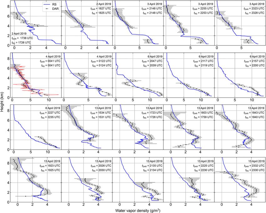
1086                JOURNAL OF ATMOSPHERIC AND OCEANIC TECHNOLOGY                                                VOLUME 37

been demonstrated, though at the expense of informa-            volumes. The next higher-frequency line location is
tion content loss relative to clear sky (Turner and             183 GHz, implying that developing such a DAR system
Löhnert 2014).                                                  also requires G-band radar innovation. While this re-
   The need for improved spaceborne observation of              quirement brings added technical complexity, it prom-
vertical water vapor profiles is recognized by the scientific   ises added benefits for developing such a system, as
community, with the recent decadal survey [National             G-band radar opens new remote sensing opportunities
Academies of Sciences, Engineering, and Medicine                for studies of cloud microphysics (Battaglia et al. 2014),
(NASEM); NASEM 2018] naming the planetary                       especially in the context of multifrequency radar ob-
boundary layer (PBL) as a targeted observable, and              servations. Furthermore, the short radar wavelength
specifically calling for incubation of new space-capable        gives G-band DARs increased sensitivity to small cloud
technologies that can provide thermodynamic profiles            particles, allowing for profiling in a wide variety of cloud
near the surface with a vertical resolution of 200 m or         scenes and precipitation.
better. Active remote sensing techniques are the most              In this work, we report on the validation of ground-
promising solution to this observational problem, as            based, G-band DAR measurements of vertical water
their vertical resolution is not fundamentally limited          vapor profiles inside of clouds, as well as measurements

                                                                                                                               Downloaded from http://journals.ametsoc.org/doi/pdf/10.1175/JTECH-D-19-0122.1 by guest on 17 August 2020
by broad weighting functions near the surface as in the         of column-integrated water vapor between the surface
case of passive sounders. Differential absorption lidar         and cloud base. The instrument, called the Vapor In-
(DIAL) and differential absorption radar (DAR) hold             Cloud Profiling Radar (VIPR), features hardware up-
particular promise for increasing spatial resolution of         grades that significantly increase the radar’s sensitivity
water vapor observations because of their precise height        relative to our previous work (Roy et al. 2018) in which
registration capabilities, and increasing accuracy be-          the DAR technique was demonstrated, but not vali-
cause of the direct spectroscopic nature of the mea-            dated with ancillary water vapor measurements. We
surement (Nehrir et al. 2017). In fact, the two techniques      observe continuous cloud profiles and retrieve continu-
are highly complementary because DIAL systems, such             ous water vapor profiles from the surface to above 10 km
as the nascent High Altitude Lidar Observatory (HALO)           in height. Using an improved DAR inverse algorithm
being developed at NASA Langley Research Center                 that incorporates systematic uncertainties into the re-
(Nehrir et al. 2017), can measure water vapor profiles in       trieval, we present the first-ever validated, remotely
clear air using aerosol and molecular backscatter, but          sensed measurements of water vapor inside of clouds,
cannot profile in cloudy volumes. DAR, on the other             and demonstrate strong agreement between DAR and
hand, relies on cloud hydrometeors in order to derive           in situ humidity measurements within the PBL and free
the differential absorption signal, and thus increases in       troposphere.
precision as cloud amount increases, provided the signal
is not too severely attenuated.
                                                                2. Instruments and measurement methods
   While DIAL is a long-established technique for both
ground-based (Browell et al. 1979; Nehrir et al. 2011;            The validation measurements described in this work
Spuler et al. 2015; Weckwerth et al. 2016) and airborne         were performed during an intensive observation period
(Browell et al. 1998) water vapor profiling measure-            on site at the ARM Southern Great Plains (SGP) central
ments, DAR is a recently emerging humidity remote               facility from 2 to 14 April 2019. The primary measure-
sensing technology that utilizes a wideband radar trans-        ments used for DAR humidity validation are radiosonde
mitter to measure cloud and precipitation reflectivity          humidity profiles, since existing humidity remote sens-
profiles at multiple frequencies near an H2O rotational         ing systems are unreliable inside of clouds. Additionally,
absorption line. Additionally, DAR has been investi-            water vapor profiles from the ARM Raman lidar allow
gated in recent instrument simulator studies showing            for high-temporal-resolution comparisons with DAR
promise for spaceborne water vapor measurement ap-              measurements of integrated water vapor (IWV) between
plications (Lebsock et al. 2015; Millán et al. 2016;            the surface and cloud base.
Battaglia and Kollias 2019). Unlike wavelengths for
                                                                a. G-band DAR: VIPR
DIAL systems, where many atmospheric gases feature a
plethora of ro-vibrational transitions (e.g., H2O, CH4,            VIPR is a proof-of-concept DAR being developed at
and CO2), the microwave and millimeter-wave spectrum            the Jet Propulsion Laboratory (JPL) for remote sensing
features only a handful of absorption lines from O2 and         of water vapor in cloudy volumes, specifically targeting
H2O. While it has been proposed to utilize the water            the PBL. In addition to being the first water vapor DAR,
vapor line at 22 GHz for DAR (Meneghini et al. 2005),           VIPR is the first all-solid-state G-band cloud radar, and
such a system would be limited to sampling precipitating        is operated in frequency-modulated, continuous-wave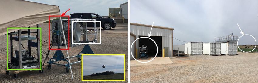
JUNE 2020                                          ROY ET AL.                                                          1087

(FMCW) mode to increase the transceiver sensitivity          TABLE 1. VIPR hardware and radar signal acquisition parameters.
relative to a pulsed system. An early version of the
                                                                                    Transmitter/receiver
VIPR system, discussion of FMCW radar detection,
                                                             W-band input power                             1.6 W
and demonstration of the DAR measurement principle
                                                             G-band output power                            0.2 W
were previously described in detail in Cooper et al.         System noise figure                            10 dB
(2018) and Roy et al. (2018). Since this early work, a       Antenna diameter                               0.6 m
higher-power transmitter and higher-gain optics have         3 dB beamwidth                                 0.248
been installed, greatly increasing the sensitivity of the    Antenna gain (calculated)                      58 dB
                                                             Beam polarization                             Circular
system, and the hardware has been modified for aircraft
deployment. Technical details of the aircraft-compatible                Nominal radar signal acquisition parameters
VIPR system can be found in Cooper et al. (2020),            Online frequency                              174.8 GHz
while relevant details of the instrument hardware for        Offline frequency                              167 GHz
this work are discussed below and summarized in              Transmitter frequency                           80 Hz
                                                               switching rate
Table 1. Figure 1 shows VIPR during the ARM SGP
                                                             Reflectivity detection sensitivity   240 dBZ for SNR 5 1 at 1 km
deployment in both calibration and cloud-measurement

                                                                                                                                Downloaded from http://journals.ametsoc.org/doi/pdf/10.1175/JTECH-D-19-0122.1 by guest on 17 August 2020
                                                             Time-domain window                             Hann
configurations.                                              Range sidelobe suppression                    223 dB
  The radar features a state-of-the-art, all-solid-state     Number of chirps per frequency                  2000
transmitter that is tunable between 167 and 174.8 GHz        Chirp duration                                  1 ms
                                                             Chirp bandwidth                               10 MHz
with 200 mW of CW output power, leveraging significant
                                                             Range resolution                                15 m
research and development in high-power millimeter-           Radar duty cycle                                80%
wave generation at JPL using GaAs Schottky diode
frequency multiplication technology (Siles et al. 2018).
The chosen radar band is a result of international reg-
ulations [National Telecommunications and Information        time-domain signal, resulting power spectra, and 2D
Administration (NTIA); NTIA 2015] that prohibit              plots of cloud reflectivity. Digital signal processing steps
G-band transmission in spectral regions reserved for         include the application of a time-domain window to a
passive satellite sensors, including the 174.8–191.8 GHz     buffered set of 400 radar pulses, computation of indi-
band used for humidity sounding. As a result, VIPR is        vidual power spectra using fast Fourier transforms
positioned on the low-frequency flank of the 183 GHz         (FFTs), and averaging of the resulting power spectra.
water vapor absorption line, which makes the system          For memory considerations, spectral averages are
primarily sensitive to PBL water vapor and allows the        computed for sets of 2000 pulses at each frequency
radar beam to penetrate through the whole atmosphere,        and then stored in permanent memory. For the typical
whereas frequencies closer to the line center would          acquisition parameters in Table 1, a single logged
experience too much absorption to feasibly probe all         measurement for two transmit frequencies takes 5 s,
levels. As compared with high-peak-power, pulsed             which sets the smallest time resolution for humidity
cloud radars with transmitter duty cycles on the order of    profiling, and during which we rapidly switch between
1%, the use of FMCW detection makes VIPR’s time-             transmitter frequencies at a rate of 80 Hz.
averaged output power equivalent to a 20 W pulsed sys-          Differential absorption measurements using cloud
tem. Furthermore, the short wavelength of l 5 1.8 mm,        radars feature a few important distinctions from DIAL
large primary aperture gain, and low system noise figure     systems. First, the large width of molecular absorption
result in a radar signal-to-noise ratio (SNR) of unity       lines at millimeter and submillimeter wavelengths in the
for a cloud reflectivity of 240 dBZ at 1 km range using      troposphere requires that the ‘‘online’’ and ‘‘offline’’
nominal radar acquisition parameters (see Table 1).          transmitter positions span a fractional bandwidth of
   Data acquisition and signal processing are performed      1%–10%, while for DIALs this number is typically
on a rack-mounted PC, after the FMCW radar signal has        around 0.01%. Second, the scattering targets of interest
undergone analog pulse compression in the front-end          for DAR are the hydrometeors that make up clouds and
G-band mixer and subsequent I/Q down-conversion to           precipitation, while for DIAL, the dominant lidar signal
baseband. A single computer program controls the             originates from atmospheric aerosols. Because charac-
necessary components for radar signal generation (e.g.,      teristic diameters of hydrometeor drop size distributions
chirp initiation, transmit frequency switching), digitizes   (DSDs) can vary by large amounts over small spatial
the complex I/Q baseband signal, performs digital signal     scales, these two factors make DAR susceptible to sys-
processing in parallel with radar signal acquisition, and    tematic measurement biases stemming from frequency-
provides a real-time display of the FMCW baseband            dependent scattering. Furthermore, because the observed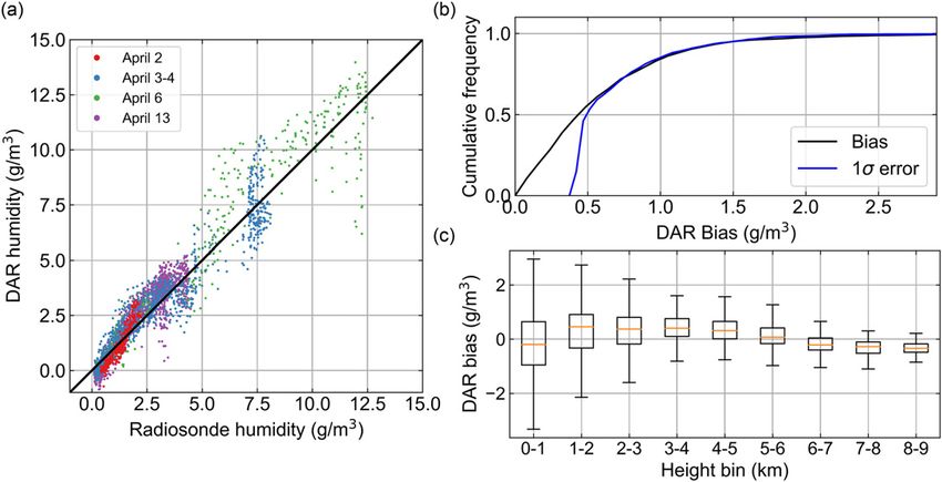
1088                 JOURNAL OF ATMOSPHERIC AND OCEANIC TECHNOLOGY                                                                 VOLUME 37

            FIG. 1. VIPR deployment at the ARM SGP site in (a) calibration sphere measurement configuration and
          (b) zenith-pointing cloud measurement configuration. The radiosonde launches, Raman lidar, and calibration
          sphere are located at the central facility, with approximate distances of 900, 610, and 460 m from VIPR,
          respectively.

                                                                                                                                               Downloaded from http://journals.ametsoc.org/doi/pdf/10.1175/JTECH-D-19-0122.1 by guest on 17 August 2020
cloud and precipitation scenes can change quickly in              Here Z(r, f) and Zobs(r, f) are the unattenuated and
time (e.g., from advection and sedimentation), it is              observed reflectivity factors,
critical to switch between DAR frequencies rapidly, as                                    ðr
otherwise temporal dependence of reflectivity would                          t(r, f ) 5        dr0 [bg (r0 , f ) 1 bh (r0 , f )]         (2)
be indistinguishable from frequency dependence and                                         0
therefore humidity.
                                                                  is the one-way optical depth, bg and bh are the gaseous
   To mitigate the potential biases from frequency-
                                                                  and hydrometeor absorption coefficients, and C( f ) is a
dependent hydrometeor scattering, we implement a
                                                                  radar hardware calibration factor. The procedure for
new DAR retrieval method that is based on a regu-
                                                                  determining C( f ) and thus calibrating reflectivity pro-
larized least squares approach and is discussed in
                                                                  files is outlined in the appendix. For DAR measure-
section 3b. Furthermore, to limit the deleterious effects
                                                                  ments of water vapor profiles inside of clouds, the value
from cloud scene dynamics we switch between transmit
                                                                  of C( f ) is not needed because the retrieval involves
frequencies after 10 pulses of 1 ms duration at each
                                                                  the ratio of Pe(r, f) at two different ranges. Thus, the
frequency. With a 2 ms switching time for the Ka-band
                                                                  relevant sources of uncertainty in the retrieval of hu-
synthesizers that generate the radar signal, this results in
                                                                  midity are the random error in the measurement of Pe
a transmitter duty cycle of 80%. We note that in recent
                                                                  and the systematic uncertainty related to the frequency-
instrument simulation work, Battaglia and Kollias (2019)
                                                                  dependent scattering parameters and stemming from
employed a retrieval that includes an extra fitting pa-
                                                                  our lack of knowledge about the true hydrometeor
rameter to independently extract the spectral dependence
                                                                  DSD. The systematic uncertainty terms will be discussed
of hydrometeor scattering and thus retrieve an unbiased
                                                                  in more detail in section 3b.
humidity. However, this requires a large transmitter
                                                                     In previous work (Roy et al. 2018), we demonstrated
bandwidth to distinguish the linear frequency depen-
                                                                  that the distribution of measured radar echo powers
dence of hydrometeor scattering from the higher-order
                                                                  follows the well-known radar speckle model for ran-
dependence of the water vapor absorption coefficient.
                                                                  domly distributed scatterers, with resulting variance
For VIPR, the transmit band from 167 to 174.8 GHz
features little curvature of the water vapor absorption                                                    !
                                                                                           P2e (r)   2  2
coefficient, and is fixed by a combination of interna-                       var[Pe (r)] 5         11 1 2 ,                              (3)
tional regulations and hardware constraints. For these                                       N       Sn Sn
validation measurements, we employ a two-frequency
differential absorption measurement approach, with                where Sn 5 Pe(r)/Pn(r) is the signal-to-noise ratio, Pn(r)
offline frequency f1 5 167 GHz and online frequency               is the receiver noise power in range bin r, and N is the
f2 5 174.8 GHz.                                                   number of independent pulses averaged to obtain the
   The primary quantity measured by VIPR is the radar             echo power estimate. In contrast to pulsed radar sys-
echo power as a function of range and frequency,                  tems, we write the noise power in FMCW radar explic-
                                                                  itly as a function of range because of the mapping of
                         Z(r, f )e22t(r,f ) Zobs (r, f )          range to frequency and the potential for nonuniform
          Pe (r, f ) 5                     5            .   (1)
                            C(f )r2          C(f )r2              gain and noise power as a function of frequency in the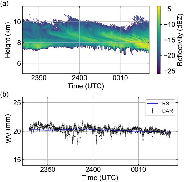
JUNE 2020                                          ROY ET AL.                                                      1089

baseband electronics. Additionally, the application          RS accuracy of 0.7, 0.4, 0.2, and 0.1 g m23 at 208, 108, 08,
of a time-domain window to the baseband radar sig-           and 2108C, respectively.
nal prior to computing the power spectrum intro-                In fact, for water vapor profiling inside of clouds, the
duces covariance between neighboring range bins.             RS in situ measurement is the only reliable one out of all
The specific form of this covariance term can be de-         the ARM instruments, since existing passive and active
rived by invoking the convolution theorem, which             remote sensors are incapable of making this measure-
allows one to express the complex Fourier ampli-             ment accurately. However, for the measurements of
tudes of the windowed time-domain signal as a linear         IWV between the surface and cloud base, we utilize
combination of those from the unwindowed signal,             water vapor profiles retrieved using the ARM Raman
which themselves are statistically independent. The          lidar (RL) in addition to the RS values (Turner et al.
mean values and covariance matrix for the radar echo         2016). The RL transmits a near-UV (355 nm), high-
power spectrum are then computed using the squared           peak-power pulse, and detects the inelastically scattered
moduli of the windowed amplitudes. For the Hann              photons from particular H2O and N2 vibrational tran-
window used in this work, nearest neighbors have             sitions. The range-resolved ratio of detected inelastically
covariance                                                   scattered photons from H2O and N2 provides a profile

                                                                                                                            Downloaded from http://journals.ametsoc.org/doi/pdf/10.1175/JTECH-D-19-0122.1 by guest on 17 August 2020
                                                  !          that is proportional to the water vapor mixing ratio,
                             4P2e,6     2     2              with a multiplicative constant provided by an ancillary
  cov[Pe (r), Pe (r 6 Dr)] 5        11     1        , (4)
                               9       Sn,6 S2n,6            sensor for absolute calibration (Whiteman et al. 1992;
                                                             Turner and Goldsmith 1999). The spatial and temporal
where Pe,6 5 [Pe(r) 1 Pe(r 6 Dr)]/2, Sn,6 5 2Pe,6/[Pn(r) 1   resolution of the water vapor product used here are 60 m
Pn(r 6 Dr)], and Dr is the radar range resolution. In        and 10 s (ARM 2015). In between radiosonde launches
FMCW radar, the range resolution is given by Dr 5            the RL provides valuable independent water vapor
c/2DF, where c is the speed of light and DF is the fre-      profiles with high temporal resolution that we utilize in
quency chirp bandwidth. In this work, the nominal chirp      the IWV measurement comparisons.
bandwidth of DF 5 10 MHz results in a range resolution
of Dr 5 15 m. Therefore, the measurement covariance
                                                             3. Retrieval methodology
matrix, which we will need for the regularized least
squares retrieval in section 3b, is tridiagonal.                The DAR humidity measurement principle is to use
                                                             the spectral variation of Zobs(r, f) and known absorption
b. ARM instruments
                                                             line shape to estimate the water vapor density along
   The primary measurement used for DAR humidity             the beam path. With continuous profiles of reflectivity
validation comes from the radiosondes (Vaisala RS41-         over an extended range (e.g., from clouds and precipi-
SG) launched from the ARM SGP central facility,              tation), one can use Zobs measurements at two ranges
located about 900 m NW of the radar’s location. In addi-     r1 and r1 1 R to remove the absorption contribution
tion to the nominal ARM radiosonde (RS) launches at          between the radar and r1 as well as the dependence on
0000, 0600, 1200, and 1800 UTC, there was an increased       radar calibration, and thus retrieve the average absolute
frequency of RS launches as high as twice per hour when      humidity between these two ranges. Alternatively, if
thick clouds were present. The typical ascent rates were     there is a measurement at a single range (e.g., Earth’s
between 5 and 7 m s21, and temperature, relative hu-         surface for an airborne DAR or a cloud base for a
midity (RH), and GPS height were recorded every sec-         ground-based system), knowledge of the relative radar
ond. In this work, we report all height coordinates          calibration for all transmitted frequencies allows for a
referenced to mean sea level. The radiosondes quickly        measurement of the corresponding IWV.
advected away from the ARM site after launch with an            In the case of the two-range measurement, varying the
average horizontal displacement of 30 km at 10 km            starting position r1 throughout the cloud returns the
height. While this introduces the potential for colloca-     full in-cloud water vapor profile, with effective resolu-
tion errors between in situ and remotely sensed mea-         tion R. If the retrieval resolution is coarser than the ra-
surements, we find that humidity profiles from RS            dar range resolution, that is, if R . Dr, this approach
launches spaced 30 min apart show little variation on the    leads to oversampling of the humidity profile. Ideally,
scale of DAR humidity errors. Therefore, in our analysis     one would set R equal to the radar range resolution to
we treat the entire profile measurement as having            maximize the humidity profile resolution. However,
occurred at the time of launch. From the RH and              several constraints on DAR systems make it the case
temperature accuracy values reported on the Vaisala          that R is typically greater than Dr. First, the difference
RS41-SG datasheet, we calculate an absolute humidity         in absorption cross section at the online and offline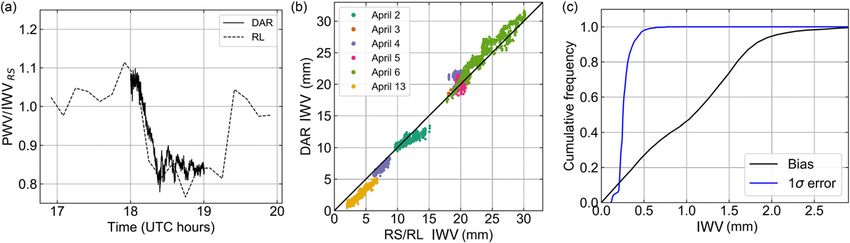
1090                  JOURNAL OF ATMOSPHERIC AND OCEANIC TECHNOLOGY                                                                VOLUME 37

frequencies and desired humidity accuracy set the                   coefficient. In this work, we calculate gaseous absorp-
achievable resolution R, which in the case of VIPR is               tion parameters using the millimeter-wave propagation
constrained by the allowable transmission band. In                  model from the EOS Microwave Limb Sounder (Read
fact, this consideration suggests the use of nonuniform             et al. 2004). Making the assumption that the spatial
vertical spacing in the retrieved humidity profile, with            variation of ky and bg,d is small on the scale R, we re-
resolution decreasing as a function of altitude due to the          place their values in the integrand in Eq. (5) with those
smaller differential absorption cross section. However,             at the midpoint r 5 (r1 1 r2 )/2 and evaluate the integral
in this work we adopt uniform vertical spacing to sim-              to yield
plify the analysis and because we anticipate averaging
the retrieved profiles in time to increase precision.               g(r1 , r2 , f ) 5 a(r1 , r2 , f ) 1 ry ky (r, f ) 1 bg,d (r, f ) 1 bh (f ) ,
Second, radar speckle noise presents a fundamental                                                                                           (6)
limit on the reflectivity precision within a single range
bin even for infinite SNR. Thus, it is desirable to use the         where a 5 (2R)21 ln[Z(r1, f)/Z(r2, f)] and ry and bh
smallest range bin size possible and therefore acquire              are the average values of the respective quantities
more independent power samples. While one could                     between r 1 and r 2 . Next, we perform a Taylor ex-

                                                                                                                                                   Downloaded from http://journals.ametsoc.org/doi/pdf/10.1175/JTECH-D-19-0122.1 by guest on 17 August 2020
subsequently average adjacent range bins down to the                pansion of hydrometeor scattering quantities Z and
resolution R, cloud reflectivities can easily vary by more          bh , which involve integrations of single particle
than an order of magnitude over the scale of the                    scattering parameters over a DSD, and retain only
achievable humidity resolution R, and therefore, such               the first-order frequency dependence because of the
averaging erases information that could be utilized in              small fractional bandwidths used for DAR systems
the retrieval.                                                      (1%–10%). Note that the equivalent parameters for
  In this section, we present a new DAR inversion                   DIAL systems can be taken to be independent of
method that retrieves the humidity profile at the                   frequency because of the extremely small fractional
downsampled resolution R while utilizing all reflectivity           bandwidths involved.
measurements at resolution Dr, resulting in no over-                  Thus, the standard DAR retrieval amounts to per-
sampling of the humidity profile. Furthermore, the least            forming a least squares fit of the function
squares approach employed in this retrieval simplifies
the accounting of covariance terms between adjacent                    ^ 5 a1 1 a2 3 (f 2 f1 ) 1 a3 3 ky (r, f ) 1 bg,d (r, f )
                                                                       g                                                                     (7)
ranges, and allows for the inclusion of systematic un-
certainty as well as regularization to mitigate the po-             to the data, with the fitting parameters having the physical
tential biases from frequency-dependent scattering.                 interpretations a1 5 a(r1 , r2 , f1 ) 1 bh (f1 ), a2 5 (›/›f )(a 1
Below we summarize the standard retrieval approach                  bh )jf1 , and a3 5 ry , where f1 is a reference frequency
for differential absorption measurements to provide                 within the transmitted band. Seemingly, then, mea-
context before presenting the new algorithm.                        surements of Zobs at three different frequencies should
                                                                    suffice to fully determine these coefficients and re-
a. Standard differential absorption retrieval
                                                                    trieve unbiased humidity estimates. However, if ky is
  The standard DAR approach (Roy et al. 2018;                       nearly linear across the range of frequencies used, then
Battaglia and Kollias 2019) begins by combining the                 a2 and a3 become degenerate fitting parameters, and
observed reflectivities to form the observed absorption             the choice of including a linear term leads to an infla-
coefficient                                                         tion of the estimated humidity variance. Clearly, the
                          "               #                         measurement in this case cannot distinguish between
                      1     Zobs (r1 , f )
   g(r1 , r2 , f ) 5    ln                                          frequency-dependence due to humidity and hydro-
                     2R     Zobs (r2 , f )                          meteor scattering. Hence, DAR retrievals will be most
                          "            #     ð                      accurate when ky exhibits strong curvature with re-
                      1     Z(r1 , f )      1 r2 0
                   5    ln               1       dr [bg (r0 , f )   spect to frequency. Unfortunately, however, ky has
                     2R     Z(r2 , f )      R r1
                                                                    very little curvature across the transmission band used
                  1 bh (r0 , f )],                           (5)    in this work, and so utilizing the standard DAR re-
                                                                    trieval would require setting a2 5 0. The frequency-
where r2 2 r1 5 R. Next, we write bg(r, f) 5 ry(r)ky(r,             dependent hydrometeor terms would then enter directly
f) 1 bg,d(r, f), where ry is the water vapor density, ky            as a bias. As shown in the next section, we attempt
is the mass extinction cross section including contri-              to limit these biases by retrieving the entire humidity
butions from all H2O absorption lines (i.e., the con-               profile in a single regularized least squares minimization
tinuum contribution), and bg,d is the dry-air absorption            routine.
JUNE 2020 ROY ET AL. 1091
b. Regularized least squares approach to account for spatial distribution of the cloud micro-
physical properties (e.g., DSD parameters) as well as
In this section, we present a new retrieval algorithm
atmospheric parameters of temperature, pressure, and
for the case of two transmitted frequencies, f1 and f2, in
humidity. However, the DAR approach is powerful
which the entire humidity profile and corresponding
because it is largely insensitive to all of these details
covariance matrix are estimated in a single least squares
except for the humidity. Thus, we want a forward model
minimization procedure, in contrast to previous ap-
that amounts to a fully determined linear system of
proaches that iteratively retrieve the humidity at each
equations, as is the case for the standard differential
height (Roy et al. 2018; Battaglia and Kollias 2019). This
absorption retrieval [Eq. (7)]. We accomplish this by
approach has the additional advantage of being ame-
choosing the state vector elements to be x 5 [x1, x2],
nable to regularization methods that constrain the form
where [x1]i 5 ln{[Zr(f1)]i/Z0} and Zr(f1) 5 [Zr(r1, f1),
of the retrieved profile. The extension of this method to
Zr(r2, f1), . . . , Zr(rN, f1)] consists of the retrieved re-
arbitrarily many frequencies is straightforward.
flectivities at one of the transmitted frequencies and
We begin the formulation of the least squares re-
includes attenuation from hydrometeors, but not gas-
trieval by defining the measurement vector y 5 [y1, y2],
eous attenuation, and x2 5 ry consists of the humidity
Downloaded from http://journals.ametsoc.org/doi/pdf/10.1175/JTECH-D-19-0122.1 by guest on 17 August 2020
where [yj]i 5 ln[Zobs(ri, fj)/Z0] and r 5 [r1 , r2 , . . . , rNr ] is
values to be retrieved at ranges rr 5 [rr,1, rr,2, . . . , rr,M].
the collection of radar ranges for which the reflectivity
Because of the potential sparsity of the observed
measurements at all frequencies have SNR greater than
reflectivity profile, the definition of the retrieved hu-
some threshold value. For the in-cloud humidity profile
midity profile ry and its corresponding range axis re-
retrievals presented in this work, we set this threshold to
quires some care. To maximally utilize the information
1. The measurement vector therefore has length 2Nr.
in the measurements, we want the retrieval to both
The choice of using the logarithm of reflectivity, and not
profile inside of continuous cloud volumes with reso-
linear units, in the measurement vector ensures that the
lution R and return IWV values in between cloud
forward model is linear in the humidity, and is justified
boundaries as well as between the radar and first cloud
so long as the relative error of the Zobs measurement is
signal. Previous DAR retrieval methods based on fixed
small. For the measurements presented in this work,
differencing in space of measurements separated by R
this condition is satisfied due to the large number of
lose the ability to extract information between cloud
pulses N 5 2000 averaged at each frequency, with a
layers with large separations. As we will see, this prob-
relative error of 0.25% for an SNR of 1. The resulting
lem is naturally avoided when using the least squares
measurement covariance matrix is block diagonal,
solution approach, since the entire humidity profile is
since the measurement errors at different frequencies
retrieved from a minimization problem in which the
are uncorrelated, with Sy 5 diag(Sy1 , Sy2 ). To determine
forward model interpolates between all humidity
the form of each individual block, we first calculate the
points, and not just those separated by R. Anticipating
covariance matrix for the reflectivity vector z 5 [Zobs(f1),
that we will want to build up time series of humidity
Zobs(f2)], and then transform to the measurement space
profiles with regular gridding in space, we enforce that
according to Sy 5 Jz Sz JTz , where Sz 5 diag[SZ( f1),
the humidity positions be of the form rr,i 5 niR for some
SZ(f2)] is the covariance matrix for z and Jz is the
integer ni. Then, given a measurement range vector r
Jacobian of y with respect to z. The individual covari-
with maximum value rmax, we form rr by retaining all
ance matrices for observed reflectivity measurements
values ni for which there is at least one element of r
are themselves tridiagonal, with
in the interval [(ni 2 1/2)R, (ni 1 1/2)R). Additionally,
[SZ (fi )]jk 5 C2 (fi )rj2 frj2 var[Pe (rj )]djk we always include the surface point ni 5 0 as the first
entry in rr.
1 rk2 cov[Pe (rj ), Pe (rk )](dj,k11 1 dj,k21 )g, (8) The first step in constructing the forward model is
to interpolate the lower-resolution humidity profile
where the power variance and covariance terms are to the radar range resolution Dr, giving a new hu-
defined in Eqs. (3) and (4), and d is the Kronecker delta. midity vector r ~ with range axis ~r 5 [0, Dr, 2Dr, . . .].
Note that if adjacent elements of the measurement Next, we use profiles of temperature and pressure at
vector do not correspond to adjacent radar range bins the same Dr resolution to calculate the resulting gas-
(i.e., if jrj 2 rkj 6¼ Dr), then the off-diagonal term is zero. absorption optical depth vector t~g 5 [~ t g (f1 ), t~g (f2 )]
Next, we must define the state vector x and forward according to
model F(x, b), where b is a vector of parameters that are
t~g,i (fj ) 5 t~g,i21 (fj ) 1 Dr[bg,d (~ ~ i21 ky (~
ri21 , fj ) 1 r ri21 , fj )],
input to the forward model, but not retrieved. A full
radiative model for the beam propagation would need (9)1092 JOURNAL OF ATMOSPHERIC AND OCEANIC TECHNOLOGY VOLUME 37
with t~g,0 5 0. Note that the gas absorption dependence
on temperature and pressure are implicit in the r~ de-
pendence. For the retrievals presented in section 4, we
use the radiosonde surface measurements and assume
hydrostatic balance with a 6.58C km21 lapse rate to
calculate the temperature and pressure profiles. Last,
the calculated optical depth vector is then masked to
only include values at the measured range positions r,
yielding the vector tg of length 2Nr. The recursive re-
lationship in Eq. (9) can be cast as a matrix equation of
the form
tg 5 Tr y 1 t g,d , (10)
FIG. 2. Ratio of reflectivity at f2 5 174.8 GHz and f1 5 167 GHz
for liquid water spheres at 280 K, integrated over a modified
which will be necessary for the matrix inversion solu-
Downloaded from http://journals.ametsoc.org/doi/pdf/10.1175/JTECH-D-19-0122.1 by guest on 17 August 2020
gamma DSD for four different shape parameters n.
tion to the regularized least squares problem. Here t g,d
is a constant vector of dry air optical depths, and T is a
2Nr 3 M matrix. It is important to note that for DAR humidity pro-
The forward model is then defined as F(x, b) 5 [F(x, b, filing, systematic biases stemming from frequency-
f1), F(x, b, f2)], where dependent backscattering would only arise if di varies
in range. In the context of this retrieval, then, it is clear
[F(x, b, f1 )]i 5 ln[Zr (ri , f1 )/Z0 ] 2 2t g,i (f1 ) , that our choice of constant d will not correct for these
[F(x, b, f2 )]i 5 ln[di Zr (ri , f1 )/Z0 ] 2 2t g,i (f2 ) , (11) potential biases. However, this formulation gives us a
way to propagate our uncertainty about these effects
and di is a fixed scaling factor that accounts for differ- into our eventual estimates of humidity. Specifically,
ential backscattering coefficients between the two fre- imperfect knowledge of the forward model parameters
quencies. Using Eq. (10) and the definition of x, we can b can be represented by a systematic error covariance
write the forward model as matrix in the measurement space according to (Rodgers
2000) Se 5 Jb Sb JTb , where Sb 5 s2d INr and Jb is the 2Nr 3
F(x, b) 5 Kx 1 b , (12) Nr Jacobian of the forward model with respect to b. It is
easy to show that the resulting Se is a 2Nr 3 2Nr diagonal
where matrix with [Se]ii 2 (sd/d)2 for i . Nr, and [Se]ii 5 0 for
#
" i # Nr. It may appear that, because Zobs(r, f) ‘ C( f ), the
IN measurement error ought to include uncertainty in the
K5 r
T (13)
IN determination of C( f ). However, a miscalibrated value
r
of C( f ) will only affect the water vapor measurement
is defined in block form, INr is the Nr 3 Nr identity ma- between the radar and the first echo range, with subse-
trix, and b includes both the di and t g,d terms. For this quent retrieved humidity values being completely in-
work, we choose the same value d for all di, informed by sensitive to this factor. Therefore, we do not include
Lorenz–Mie calculations of liquid hydrometeor scat- calibration uncertainty in the measurement covariance
tering (Bohren and Huffman 2004). This is equivalent analysis, and will discuss the related column-integrated
to assuming that the DSD characteristic diameter is water vapor issues in the next section.
constant in space. The range of d values for different Finally, in order to mitigate the humidity biases that
DSDs is shown in Fig. 2, where we assume a modified arise from the linear term in Eq. (7), we implement a
gamma distribution as in Roy et al. (2018) and vary the regularization term. We begin by noting that these bia-
shape parameter n from 1 to 4 to explore the sensitivity ses often occur over short spatial scales, for instance due
to the assumed DSD shape. Focusing on the n 5 4 case, to the differential backscattering at a boundary between
which is a typical value used for nonprecipitating clouds, intense and light precipitation, or between precipitation
we see that the range of characteristic diameters over and a cloud base, and thus tend to produce large, un-
which b varies the most is 10 2 100 mm. To be conser- physical gradients of water vapor in the retrieved profile.
vative, we pick for our value of b the average of the two A natural regularization term to utilize, then, is one that
limits in Fig. 2, or d 5 0.9, and assign a systematic un- penalizes sharp gradients in the retrieved state. For this
certainty of sd 5 0.1. term, we choose the sum of squared discrete derivativesJUNE 2020 ROY ET AL. 1093
of the humidity vector, which can be written as a qua- Because the forward model is linear in the state vec-
dratic form tor, the minimization problem [Eq. (15)] can be solved
!2 by means of a matrix inversion,
M21
ri11 2 ri x 5 [KT (Sy 1 Se )21 K 1 lreg A]21 KT (Sy 1 Se )21 (y 2 b) .
^
x T
Ax 5 d22
r å rr,i11 2 rr,i
(14)
i51
(17)
for some matrix A, where dr is some chosen scale for Furthermore, the retrieved state covariance matrix is
penalized humidity gradients, and is set to 10 g m23 km21 given by the Hessian of C (x),
in this work. The inverse algorithm is then the solution
to a least squares minimization problem, ^ 5 [KT (S 1 S )21 K 1 l A]21 .
S (18)
x y e reg
^
x 5 argminC (x) , (15) We note here that the regularization term is not intro-
x
duced because of ill-posedness of the unregularized
where the cost function is given by problem, as is the case with the introduction of the
Downloaded from http://journals.ametsoc.org/doi/pdf/10.1175/JTECH-D-19-0122.1 by guest on 17 August 2020
prior distribution in optimal estimation (Rodgers
C (x) 5 [y 2 F(x, b)]T (Sy 1 Se )21 [y 2 F(x, b)] 2000), but rather to constrain the form of the retrieved
profile. From the form of S ^ x in Eq. (18), it becomes
1 lreg xT Ax, (16) apparent that inclusion of the systematic error covari-
ance matrix Se can be viewed as effectively inflating
and lreg $ 0 is a dimensionless parameter that deter- the measurement variance. To get a sense of the scale of
mines how severely to penalize humidity gradients. To this variance inflation, we utilize the fact that the diag-
implement the gradient regularization scheme, we need onal elements of Sy are equal to the squared relative
to find the symmetric matrix A that satisfies Eq. (14). error of the corresponding echo power measurement,
One can show that A is block diagonal and of the form var[Pe (r, f )]/P2e (r, f ), and those for Se are either zero or
T 22
A 5 diag(0Nr , d22
r D Dr D), where the first block is a equal to (sd/d)2. Thus, using Eq. (3) for the measure-
Nr 3 Nr matrix of zeros, [D]ij 5 di,j21 2 di,j is a (M 2 1) 3 ment relative error with N 5 2000 pulses, we see that this
M finite differencing matrix, and [Dr]ij 5 di,j(rr,i11 2 rr,i) approach amounts to an increase in variance by a factor
is a (M 2 1) 3 (M 2 1) diagonal matrix. We set the of about 20 for high-SNR measurements, and by a factor
regularization parameter lreg 5 1, which amounts to a of about 4 for measurements with SNR 5 1.
conservative penalty of gradients on the scale dr. This
gradient regularization method is similar in nature to c. Column-integrated water vapor
applying a spatial low-pass filter to the retrieved hu- The IWV measurement between the surface and an
midity profile, but performs the smoothing as part of a elevated cloud base is an analogous measurement to
single least squares optimization routine, works for future column measurements made from an airborne
nonregularly spaced points, and naturally allows for platform between the radar and the surface. These
uncertainty quantification in the retrieved, smoothed measurements are of interest for any DAR because in
quantities. [An example scenario where this profile- the absence of clouds, the surface return is the only radar
smoothing approach is particularly effective is shown measurement acquired. For the case of a single-range
in Fig. 4 (second row, left panel).] Here the red curve measurement at two frequencies, one can solve for the
represents the standard two-frequency DAR re- IWV between the radar and range r:
trieval employed in Roy et al. (2018), which exhibits ( " # " #
significant biases due to spatially varying hydrome- 1 Pe (r, f1 ) C(f1 )
IWV 5 ln 1 ln
teor properties, while the regularized least squares 2hDky i Pe (r, f2 ) C(f2 )
approach successfully mitigates these effects. We note " # ðr )
that the value of dr is chosen as a compromise between Z(r, f2 ) 0 0
1 ln 2 2 dr Dbh (r ) , (19)
limiting biases that appear as sharp humidity gradients Z(r, f1 ) 0
and avoiding an overly constraining low-pass filter, Ðr
and that using 10 g m23 km21 results in good agreement where IWV 5 0
dr0 ry (r0 ),
between the median retrieval error and median bias ðr
with respect to radiosonde measurements (Fig. 5b). dr0 ry (r0 )Dky (r0 )
Because of this choice, the retrieval will smooth out hDky i 5 0 ðr , (20)
real humidity variations that are on the scale of dr dr0 ry (r0 )
or larger. 01094 JOURNAL OF ATMOSPHERIC AND OCEANIC TECHNOLOGY VOLUME 37
Dky(r) [ ky(r, f2) 2 ky( r, f1), and Dbh(r) [ bh(r, f2) 2 multiple days within the 2–14 April 2019 window. Three
bh(r, f1). The first term in Eq. (19) will have an associated example datasets with significant spatiotemporal cloud
random error, while the remaining three may introduce coverage are presented in Fig. 3. We present the ob-
systematic error. In this work, we only utilize measure- served reflectivity measurements at f1 5 167 GHz for
ments with negligible hydrometeor content between the which SNR . 1. These 2D plots have the nominal radar
surface and r and therefore can neglect the last term in time resolution of about 5 s, and range resolution of
this equation dealing with differential absorption from 15 m. For these and all subsequent plots, the height is
hydrometeors. Using hDkyi ’ 0.25 dB km21 g21 m3, referenced to mean sea level, with the ground level at
which is representative of lower-tropospheric conditions, ARM being 0.3 km. While there is no near-range dead
we see from Eq. (19) that errors in the individual bias zone in FMCW radar, we do not use reflectivity mea-
terms of 1 dB lead to a IWV bias of 2 mm. surements within the first 100 m, because these correspond
To assess VIPR’s ability to accurately measure column- to the antenna near field and the calibration measurements
integrated water vapor, we perform a set of retrievals in were performed in the far field. Depending on the level of
which the surface-to-cloud-base IWV is the only hu- precipitation at the surface, VIPR is either positioned
midity quantity retrieved. We assume that the water outside pointing at the zenith, or just inside the facility
Downloaded from http://journals.ametsoc.org/doi/pdf/10.1175/JTECH-D-19-0122.1 by guest on 17 August 2020
vapor density decays exponentially in the vertical with a pointing between 208 and 308 off zenith. The measure-
scale height of 2 km, which is consistent with previous ments presented in Fig. 3 account for these adjustments
measurements at the ARM SGP site (Turner et al. in pointing angle.
2001). For these retrievals, we lower the nominal SNR There are two features in the reflectivity datasets to
threshold to 0.5, and in some cases to 0.25 if there are no highlight. First, there is a signature of the melting layer
returns with SNR . 0.5, allowing for IWV measure- via an abrupt reflectivity change at a persistent height on
ments using cloud layers with weak reflectivities, and each of the three days once precipitation is initiated, as
utilize reflectivity measurements within a distance R of we would expect for the cold rain process within the
the bottom cloud edge. The main reason for performing stratiform anvils associated with deep convective clouds.
a separate set of IWV retrievals, as opposed to using the Second, there is a clear impact on the maximum de-
corresponding value from the profiling retrieval detailed tectable range in the presence of precipitation, due to
in the previous section, is that the latter occurs on a the greatly increased hydrometeor absorption experi-
fixed, equally spaced vertical grid. Therefore, depending enced by the radar beam. Additionally, note that be-
on where the cloud base falls within a vertical grid cell cause the PBL humidity on 13 April is less than half that
of size R, the profiling retrieval will utilize a different on the previous days, the upper-tropospheric clouds
number of reflectivity measurements to estimate the appear to have a larger reflectivity as the beam ab-
surface-to-cloud-base IWV, and thus have variable sorption from water vapor is greatly reduced. In fact, for
sensitivity. Furthermore, we change the scaling factor both of these reasons it is clear why DAR measurements
for differential backscattering between f1 and f2 from from an airborne or spaceborne platform will offer a
d 5 0.9 to d 5 1, since we expect scattering to be substantial increase in sampling precipitating clouds, as
of Rayleigh character near the cloud edge where re- the hydrometeors and low humidity levels aloft will not
flectivities are very weak. Unlike the case of in-cloud extinguish the beam before it reaches the strongly re-
profiling, where taking the ratio of reflectivities at two flective rain drops in the lower levels.
different ranges makes the measurement insensitive to The lower panels in Fig. 3 are the retrieved, in-cloud
the value of d, incorrect specification of this parameter humidity fields from the reflectivity measurements at
biases the IWV estimate [see Eq. (19)]. We take a 167 and 174.8 GHz (the latter are not shown). We
practical approach to determining the calibration ratio utilize a humidity profile resolution of R 5 180 m, which
C(f1)/C(f2), and choose the value that gives zero average is a factor of 12 larger than the reflectivity resolution.
IWV bias with respect to the ARM instrument ground The launch times of radiosondes from the ARM central
truth. Therefore, average biases resulting from our facility are depicted with black dashed lines. Note that
choice of d and from hydrometeor absorption are im- in-cloud humidity can only be retrieved where there are
plicitly included in the determined value of C(f1)/C(f2). measurements at both frequencies, and since f2 experi-
ences more atmospheric absorption than f1, the spatio-
4. Results and discussion temporal coverage of humidity is slightly less than that
for reflectivity at f2.
a. In-cloud humidity profiles
A close scrutiny of the corresponding reflectivity and
For validation of VIPR’s in-cloud profiling capabilities, humidity plots in Fig. 3 reveals that some regions
we utilize cloud reflectivity measurements acquired on exhibit a correlation between spatial boundaries of dBZJUNE 2020 ROY ET AL. 1095
Downloaded from http://journals.ametsoc.org/doi/pdf/10.1175/JTECH-D-19-0122.1 by guest on 17 August 2020
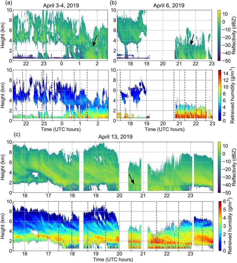
FIG. 3. Observed cloud reflectivities at 167 GHz and corresponding retrieved humidity profiles for three different
days. Dashed vertical lines correspond to radiosonde launch times. Time periods with no reflectivity measurements
are either cloud-free scenes or periods when the radar was temporarily not acquiring data. Arrows indicate the
melting-layer position.
and changes in ry. For instance, observe the marked gradient-penalty regularization scheme. Specifically, if
depression in humidity correlated with and just below the characteristic diameter of the DSD changes quickly
the melting layer position in periods with precipitation in space, we expect a large value of the second term in
in Fig. 3c, or the temporal variations of magnitude .30% Eq. (7), which can significantly bias the retrieved value
that are correlated with distinct bands of precipitation of ry. For instance, using the Lorenz–Mie calculations in
in the latter part of Fig. 3b. Comparisons of retrieved Fig. 2 for n 5 4, if the characteristic diameter varies from
humidity profiles at the nominal 5 s radar time resolution 20 to 60 mm over 180 m, there would be a resulting DAR
with radiosonde measurements show that these variations humidity bias of 5 g m23.
are not physical. In fact, such features are a manifestation While these particular variations in the retrieved hu-
of the systematic bias from differential hydrometeor midity are not random in nature, we can reduce their
reflectivity, and are the reason for implementing the effect on the accuracy of the measurement further by1096 JOURNAL OF ATMOSPHERIC AND OCEANIC TECHNOLOGY VOLUME 37
averaging vertical ry profiles in time. This will help to technique, and show the capability of VIPR to accu-
smooth out variations of the type seen in Fig. 3b, but not rately profile in-cloud humidity not only in the PBL, but
that associated with the melting layer in Fig. 3c. While throughout the troposphere.
this time-averaging procedure decreases the effective While the coincident DAR/RS measurements make
DAR ry time resolution, the situation will be much up a useful dataset for evaluating VIPR’s humidity ac-
different when VIPR is deployed from an airborne curacy, we would like to be able to use the remaining
platform. In this case, the fast aircraft motion allows 10-min-averaged profiles as well. Therefore, we linearly
VIPR to sample the spatial heterogeneities of a cloud interpolate the RS profiles in time at each height to the
scene much faster and therefore should permit a hu- DAR temporal resolution Tavg, and note the observa-
midity measurement time resolution near the nominal tion that RS humidity profiles do not change appreciably
value of 5 s. This is clear from low level of random noise in the intervals between launches (usually 0.5–2 h).
evident in the humidity fields in Fig. 3, and from the fact Furthermore, we smooth the RS profiles in height to
that the error bars in the DAR-retrieved humidity are make the effective resolution equal to that of the DAR
dominated by the introduction of the systematic error profiles by performing a convolution with a box of length
term Se, and have little contribution from the random R. The resulting comparison between remotely sensed
Downloaded from http://journals.ametsoc.org/doi/pdf/10.1175/JTECH-D-19-0122.1 by guest on 17 August 2020
measurement noise except where the SNR is low. and in situ humidity is presented in Fig. 5. The scatter-
Because the time-varying systematic biases in ry are plot in Fig. 5a has an associated correlation coefficient
not random, we must account for covariance between r 5 0.96 and RMSE of 0.8 g m23. The corresponding
adjacent time values in determining the resulting un- cumulative distribution of the absolute value of DAR
certainty. The recipe we use to compute time-averaged humidity bias relative to the interpolated RS profiles is
ry profiles involves first partitioning the 2D humidity shown in Fig. 5b. Note that we describe bias in absolute
fields into segments of duration Tavg 5 10 min. Because terms (i.e., in units of g m23) and not in terms of relative
of the sparsity of DAR datasets, it is often the case that error, because the sensitivity of a differential absorption
there are many missing data points in each segment. measurement is independent of the magnitude of ry
Therefore, we require that each segment have a mini- (Roy et al. 2018). Therefore, this approach is a more
mum of 10 measurements in order to record a final appropriate assessment of the DAR accuracy. We find
averaged humidity value. Given a set of humidity that biases are below 1 g m23 84% of the time, and below
measurements at a given height zi and between time t 2 g m23 98% of the time.
and t 1 Tavg, {ry(zi, t1), ry(zi, t2), . . . , ry(zi, tM)}, we In Fig. 5c we bin the measurements by height to assess
compute the time-average mean and variance from the bias dependence in various levels of the atmosphere,
ry (zi ) 5 M21 åj51 ry (zi , tj ) and
M
and present the resulting binned distributions as box-
plots. It is interesting to note that the variance of the
M h i bias distribution decreases with height, which at first
var[ry (zi )] 5 M22 å Sr ,i ,
y jk
(21)
seems counterintuitive given that measurement SNR is
j,k51
largest in the lowest levels of the atmosphere. However,
where the ry time covariance matrix has elements [Sry ,i]jk 5 recall that the strongest biases in the DAR humidity
sry (zi , tj )sry (zi , tk ) exp(2jtj 2 tk j/tcorr ), sry (zi , tk ) is the measurement arise from sharp spatial gradients of the
uncertainty returned by the retrieval algorithm, and characteristic DSD diameter, which are likely to occur
we set the exponential time-correlation constant to in the lower atmosphere (e.g., melting layer, localized
t corr 5 1 min. Note that because of the imposed cor- precipitation populations). Nevertheless, the near-zero
relations in the time-averaging procedure, the im- median bias in each vertical level reveals that the temporal-
provement in humidity precision with averaging time averaging approach successfully mitigates systematic
is lessp than that ffi for uncorrelated measurement aver-
ffiffiffiffiffiffiffiffiffiffiffiffiffiffi DAR biases. In future DAR measurement systems, it
aging Tavg /Dt, where Dt 5 5 s is the nominal temporal will be interesting to explore the addition of a third
resolution. transmission frequency outside of the 167–174.8 GHz
The resulting comparisons of coincident DAR and RS band to independently measure the frequency-dependent
humidity observations are presented in Fig. 4. The only hydrometeor scattering contributions to the differential
profiles excluded from this figure are those in which the absorption signal.
DAR profile spans less than 2 km. In these plots, the
b. Surface-to-cloud-base column retrievals
error bars correspond to the square root of the time-
averaged humidity variance in Eq. (21) (i.e., 1s error). We utilize all of the cloud datasets that do not feature
These are the first-ever validated measurements of wa- strong precipitation to perform a measurement of IWV
ter vapor inside of clouds using an active remote sensing between the radar and cloud base. An example cloudJUNE 2020 ROY ET AL. 1097
Downloaded from http://journals.ametsoc.org/doi/pdf/10.1175/JTECH-D-19-0122.1 by guest on 17 August 2020
FIG. 4. Comparisons of coincident radiosonde and DAR humidity profiles. The DAR profiles, which are initially retrieved with 5 s
temporal resolution, are further averaged in time to 10 min resolution for comparison with radiosonde profiles. Error bars for the DAR
measurements correspond to the square root of the variance defined in Eq. (21). For comparison, the left panel in the second row also
shows the 10-min-averaged humidity profile retrieved using the simple two-frequency DAR method from Roy et al. (2018) (red line).
scene and resulting IWV time series is presented in interpolation in time small. However, many of the da-
Fig. 6. In all of the DAR IWV measurements described tasets used for IWV measurements do not feature the
in this section, we do not perform any additional aver- same density of RS launches as those used for in-cloud
aging in time, and so the temporal resolution is 5 s. For profiling, since these were the highest-priority mea-
the RS time series (blue line in Fig. 6b), we again in- surements. Fortunately, the ARM RL performs mea-
terpolate the profiles linearly in time between launches surements of water vapor profiles in clear air every
at each height, and integrate the resulting profiles up to 10 min, and provides a valuable resource for validation
the cloud-base height determined by radar measure- of DAR surface-to-cloud-base IWV measurements.
ment. For this upper-tropospheric ice-cloud case, the However, it is often the case that the RL profiles do not
remotely sensed and in situ IWV time series agree very extend all the way to the cloud-base height detected by
well, even with the assumption of pure Rayleigh back- VIPR. Thus, we adopt an approach that merges the RS
scattering from spherical liquid hydrometeors. We note and RL water vapor information to interpolate the RS-
here that these DAR retrievals utilize the value for the integrated IWV in time with the RL temporal resolu-
radar calibration ratio C(f1)/C(f2) determined from the tion. Specifically, given an RL humidity profile we first
aggregate analysis described below. filter out values with uncertainties in excess of 2 g m23,
For the case in Fig. 6, a radiosonde was launched at resulting in a maximum RL measurement height zRL.
2330 UTC, making the potential error from linear Then, we integrate the RL and temporally interpolatedYou can also read