Long-term (1999-2019) variability of stratospheric aerosol over Mauna Loa, Hawaii, as seen by two co-located lidars and satellite measurements - ACP
←
→
Page content transcription
If your browser does not render page correctly, please read the page content below
Atmos. Chem. Phys., 20, 6821–6839, 2020
https://doi.org/10.5194/acp-20-6821-2020
© Author(s) 2020. This work is distributed under
the Creative Commons Attribution 4.0 License.

Long-term (1999–2019) variability of stratospheric aerosol over
Mauna Loa, Hawaii, as seen by two co-located lidars
and satellite measurements
Fernando Chouza1 , Thierry Leblanc1 , John Barnes2 , Mark Brewer1 , Patrick Wang1 , and Darryl Koon1
1 Jet   Propulsion Laboratory, California Institute of Technology, Wrightwood, CA, USA
2 NOAA/ESRL/Global       Monitoring Division, Boulder, CO, USA

Correspondence: Fernando Chouza (keil@jpl.nasa.gov)

Received: 26 November 2019 – Discussion started: 14 January 2020
Revised: 4 May 2020 – Accepted: 12 May 2020 – Published: 10 June 2020

Abstract. As part of the Network for the Detection of At-          sive wildfires and multiple volcanic eruptions caused a sig-
mospheric Composition Change (NDACC), ground-based                 nificant increase in stratospheric aerosol loading. This load-
measurements obtained from the Jet Propulsion Labora-              ing maximized at the very end of the time period considered
tory (JPL) stratospheric ozone lidar and the NOAA strato-          (fall 2019) as a result of the Raikoke eruption, the plume of
spheric aerosol lidar at Mauna Loa, Hawaii, over the past          which ascended to 26 km altitude in less than 3 months.
2 decades were used to investigate the impact of volcanic
eruptions and pyrocumulonimbus (PyroCb) smoke plumes
on the stratospheric aerosol load above Hawaii since 1999.         1   Introduction
Measurements at 355 and 532 nm conducted by these two
lidars revealed a color ratio of 0.5 for background aerosols       The impact of stratospheric aerosols in the Earth’s radiative
and small volcanic plumes and 0.8 for a PyroCb plume               budget and ozone burden is widely recognized (e.g., Thomp-
recorded on September 2017. Measurements of the Nabro              son and Solomon, 2009; Hofmann and Solomon, 1989).
plume by the JPL lidar in 2011–2012 showed a lidar ratio of        Their characterization is not only important to understand the
(64 ± 12.7) sr at 355 nm around the center of the plume. The       changes in atmospheric temperature and ozone profiles but
new Global Space-based Stratospheric Aerosol Climatology           has also gained relevance during recent years because of their
(GloSSAC), Cloud-Aerosol Lidar with Orthogonal Polariza-           potential use as a geoengineering tool to reduce the impact
tion (CALIOP) Level 3 and Stratospheric Aerosol and Gas            of global warming (Rasch et al., 2008). Dominated by sul-
Experiment III on the International Space Station (SAGE            fate aerosols, stratospheric aerosols are typically found in the
III-ISS) stratospheric aerosol datasets were compared to the       form of a layer that extends from the tropopause up to 35 km
ground-based lidar datasets. The intercomparison revealed a        above sea level (a.s.l.) in the tropics and about 30 km a.s.l. at
generally good agreement, with vertical profiles of extinction     midlatitudes (Hitchman et al., 1994; Kremser et al., 2016).
coefficient within 50 % discrepancy between 17 and 23 km           This stratospheric aerosol layer (SAL), also known as Junge
above sea level (a.s.l.) and 25 % above 23 km a.s.l. The strato-   layer, was discovered in 1960 by means of balloon-borne
spheric aerosol depth derived from all of these datasets shows     measurements (Junge and Manson, 1961).
good agreement, with the largest discrepancy (20 %) being             Although the stratospheric sulfur burden has been domi-
observed between the new CALIOP Level 3 and the other              nated by periodic volcanic injections of large amounts of SO2
datasets. All datasets consistently reveal a relatively quies-     and volcanic ash (Kremser et al., 2016) during past decades,
cent period between 1999 and 2006, followed by an active           some recent studies (Solomon et al., 2011) reported an in-
period of multiple eruptions (e.g., Nabro) until early 2012.       crease in the background aerosol load during less active vol-
Another quiescent period, with slightly higher aerosol back-       canic periods that could be attributed to other sources, includ-
ground, lasted until mid-2017, when a combination of exten-        ing anthropogenic SO2 emissions (Brock et al., 1995; Rollins

Published by Copernicus Publications on behalf of the European Geosciences Union.
6822                             F. Chouza et al.: Long-term variability of stratospheric aerosol over Mauna Loa, Hawaii

et al., 2018) and large wildfire-driven thunderstorms (Peter-      between 1999 and 2019 and the different optical properties
son et al., 2018).                                                 retrieved from the synergy between JPL and NOAA lidars.
   Since its discovery, several techniques have been used          Section 5 presents lidar-derived optical properties. Section 6
to monitor the evolution of the SAL, including ground-             presents an intercomparison of the two ground-based lidars
based lidars (e.g., Fiocco and Grams, 1964; Barnes and Hof-        with the three satellite-based datasets under evaluation. Fi-
mann, 2001; Trickl et al., 2013; Khaykin et al., 2017; Zuev        nally, a summary of the key findings of this paper is presented
et al., 2017), balloon-borne in situ measurements (Deshler         in Sect. 7.
et al., 2003), and satellite-borne lidars (Vernier et al., 2009)
and spectrometers (McCormick and Veiga, 1992). While
satellite-borne instruments are able to provide global cov-        2     Instruments and datasets
erage over several years, their limited lifetime requires ad-
ditional measurements that can close eventual gaps existing        2.1    JPL Mauna Loa Stratospheric Ozone Lidar
between different missions, but they can provide a common                 (MLSOL)
reference to investigate possible instrumental biases that can
arise from the difference in the measurement techniques and        The JPL Mauna Loa Stratospheric Ozone Lidar (MLSOL)
wavelengths used on each mission.                                  started its routine operations in 1993. The system is de-
   As part of the Network for the Detection of Atmo-               ployed at the Mauna Loa Observatory, Hawaii (19.53◦ N;
spheric Composition Change (NDACC), the Jet Propulsion             155.57◦ W, 3397 m a.s.l.). An extensive description of the
Laboratory (JPL) lidar group has been performing strato-           original system configuration can be found in McDermid
spheric ozone and temperature measurements at Mauna Loa,           et al. (1995). Since then, the system has undergone a few ma-
Hawaii, since 1994 (e.g., Leblanc et al., 2006; Kirgis et al.,     jor modifications and some minor technical issues. The major
2013). This long-term ground-based lidar dataset provides          modifications include the migration of the system from a mo-
not only stratospheric ozone and temperature records but           bile trailer to a building, the replacement of the Raman shift-
also a unique opportunity to evaluate current and past global      ing cell used to generate the 353 nm with a Nd:YAG laser in
stratospheric aerosol datasets. In contrast to most strato-        March 2001, and the upgrade on the data acquisition system
spheric aerosol systems, the JPL stratospheric ozone lidar         in April 2019.
operates in the ultraviolet spectral region (308–387 nm) and          In its current configuration, the system transmitter consists
has two different Raman receivers that allow the retrieval of      of a Spectra Physics PIV-400 Nd:YAG laser operating at a
aerosol extinction coefficient (αa ) profiles without the need     repetition rate of 50 Hz, followed by a third harmonic gen-
to assume a lidar ratio.                                           erator (THG), emitting pulses of about 140 mJ at 355 nm.
   Additionally, right next to the JPL ozone lidar, the Na-        For the generation of the “on wavelength” needed for the
tional Oceanic and Atmospheric Administration (NOAA)               ozone differential absorption lidar (ozone DIAL) retrieval,
has been collecting stratospheric aerosol measurements with        a set of two XeCl Excimer lasers is used. The first Excimer
a ruby-based lidar system (694 nm) since the mid-1970s and         laser (Coherent LPXpro 220) is used as an oscillator, while
with an Nd:YAG laser (532 nm) since May 1994.                      the second is used as a single-pass amplifier (Lambda Physik
   In this study, the JPL and NOAA lidars are used to inves-       LPX 220i). This configuration is operated at a repetition rate
tigate the stratospheric aerosol optical properties in the UV      of 200 Hz with a pulse energy of about 300 mJ at 308 nm.
and visible spectral regions and to evaluate three different       Both laser beams are expanded by a factor of 5 in order to
extinction profile datasets, i.e., the multi-instrument Global     reduce beam divergence and redirected to the atmosphere by
Space-based Stratospheric Aerosol Climatology (GloSSAC,            motor-controlled mirrors used for alignment purposes.
Thomason et al., 2018), the new Cloud-Aerosol Lidar with              The system receiver, mainly unchanged since the system
Orthogonal Polarization (CALIOP) Level 3 Stratospheric             description presented in McDermid et al. (1995), consists
Aerosol Profile Monthly Product (Kar et al., 2019), and the        of a 1 m aperture Dall–Kirkham telescope with a focal ra-
recently launched Stratospheric Aerosol and Gas Experi-            tio of f/8. A PARC Model 192 chopper is placed between
ment III on the International Space Station (SAGE III-ISS)         the telescope and the receiver in order to block backscat-
(Cisewski et al., 2014).                                           ter signal from altitudes below 10 km above ground level
   The paper is organized as follows. Section 2 provides a         (a.g.l.). The chopper blocking, together with the electronic
brief description of the instruments and datasets used in this     gating of the photomultiplier tubes (PMTs), helps to re-
study, including a description of the JPL and NOAA lidars          duce the signal-induced noise (SIN) generated by the strong
and the three satellite-based datasets. Section 3 describes the    backscatter from low altitudes. The system receiver consists
methods applied to the ground-based lidar datasets in order to     of six photon-counting channels: two high-intensity Rayleigh
retrieve aerosol backscatter and extinction profiles as well as    backscatter channels (355H and 308H), two low-intensity
aerosol optical depth and the corrections needed in order to       Rayleigh backscatter channels (355L and 308L), and two ni-
obtain comparable datasets. Section 4 provides an overview         trogen Raman backscatter channels (387M and 332M). Up
of the measurements conducted at Mauna Loa in the period           to April 2019, the signals were digitized with Tennelec–

Atmos. Chem. Phys., 20, 6821–6839, 2020                                              https://doi.org/10.5194/acp-20-6821-2020
F. Chouza et al.: Long-term variability of stratospheric aerosol over Mauna Loa, Hawaii                                        6823

Nucleus multichannel scaler (MCS) boards with a resolution          2.4    CALIOP Level 1B
of 300 m. Since the last system upgrade, a Licel transient
recorder with photon-counting and analog detection capabil-         The CALIOP Level 1B V4.1 (L1) data product provides half
ities has been used. The new acquisition system has a vertical      orbit (day or night) calibrated and geolocated single-shot li-
resolution of 15 m.                                                 dar profiles, including 532 and 1064 nm attenuated backscat-
                                                                    ter and a depolarization ratio at 532 nm. In this study, since it
2.2   NOAA Mauna Loa Stratospheric Aerosol Lidar                    focuses on thin stratospheric plumes, only nighttime profiles
                                                                    of attenuated backscatter at 532 nm and depolarization are
The NOAA Stratospheric Aerosol Lidar is located in the              used. Co-located MERRA-2 meteorological profiles includ-
same building as MLSOL and has been operating with its              ing temperature, pressure, and ozone concentration are also
current configuration since May 1994 (Barnes and Hof-               provided, which in this case are used as part of the aerosol
mann, 2001). The lidar is based on a Spectra Physics GCR-           backscatter coefficient retrieval process (Sect. 4.3).
6 Nd:YAG laser (30 Hz, 40 W at 1064 nm) with frequency
doubling and tripling (532 and 355 nm), although the 355 nm         2.5    CALIOP Level 3 Stratospheric Aerosol Profile
has not been used routinely. A 61 cm telescope is dedicated
to 532 nm measurements, a 61 cm telescope is dedicated to           The new CALIOP Level 3 (L3) stratospheric aerosol pro-
1064 nm, and a 74 cm telescope is dedicated to Raman nitro-         file product (Kar et al., 2019), released in August 2018, re-
gen (607 nm) and water vapor (660 nm). PMTs are used in             ports monthly mean profiles of aerosol extinction, particu-
the photon-counting mode for all channels. The system uses          late backscatter, attenuated scattering ratio (SR), and strato-
a PC 80486 and the data acquisition electronics are MCS II          spheric aerosol optical depth on a spatial grid of 5◦ in lati-
boards made by Tennelec. Measurements are made during               tude, 20◦ in longitude, and 900 m in altitude.
the night, usually once a week.                                        As part of this dataset, two different aerosol products are
                                                                    reported. One is labeled as “background” and the other is la-
2.3   The Global Space-based Stratospheric Aerosol                  beled “all aerosols”. While the first corresponds to profiles
      Climatology (GloSSAC)                                         retrieved after removing clouds, aerosols, and polar strato-
                                                                    spheric clouds (PSCs), the second only screens out clouds
The GloSSAC (data version 1.1) is a 38-year climatology             and PSCs. For this study, we use the all aerosols data prod-
of stratospheric aerosol properties based on measurements           uct from dataset version 1.0. Auxiliary atmospheric parame-
from the SAGE instruments series through August 2005 and            ters required for the aerosol extinction coefficient retrieval,
a combination of the Optical Spectrograph and InfraRed              including molecular and ozone absorption corrections, are
Imager System (OSIRIS) and CALIOP datasets thereafter               obtained from MERRA-2 (Modern-Era Retrospective anal-
(Thomason et al., 2018). The main product reported by this          ysis for Research and Applications, Version 2) (Gelaro et al.,
dataset is a series of extinction coefficient profiles at 525 and   2017). The lidar ratio assumed for the retrieval is 50 sr.
1020 nm. The data corresponds to zonally averaged extinc-
tion profiles with a latitude grid of 5◦ and a vertical grid        2.6    SAGE III-ISS
spacing of 0.5 km from 5 to 39.5 km.
   In the time frame covered by this study, the instruments         The SAGE III instrument (Cisewski et al., 2014), launched
contributing to the GloSSAC dataset are SAGE II, OSIRIS,            in February 2017 and carried by the ISS, is a moderate-
and CALIOP. In the case of SAGE II, no major processing             resolution spectrometer covering wavelengths from 290 to
is applied, as the aerosol extinction profile at 525 nm is one      1550 nm. Data collection is performed in three different
of the native data products of the instrument and the vertical      modes, namely solar occultation, lunar occultation, and limb
grid is also 0.5 km. After the end of the SAGE II mission, in       scatter measurement. The expected science products include
August 2005, and before the start of the CALIOP mission, in         vertical profiles of ozone, nitrogen dioxide, and water vapor,
August 2006, OSIRIS measurements are reported. After the            along with multiwavelength aerosol extinction.
commissioning of CALIOP, a combination of OSIRIS and                   In this study, zonally averaged extinction profiles at
CALIOP extinction profiles is provided.                             521 nm for latitudes between 15 and 25◦ N are used (data
   In the case of the CALIOP extinction coefficient calcula-        version 5.1). Native vertical grid spacing is 0.5 km.
tion, the GloSSAC dataset uses a lidar ratio equal to 53 sr
instead of 50 sr, as typically used in other stratospheric lidar
studies. This difference can be partially attributed to the dif-    3     Lidar products and data analysis
ference between the original CALIOP wavelength (532 nm)
and the GloSSAC extinction dataset, reported at 525 nm.             3.1    Backscatter coefficient retrieval

                                                                    Different approaches exist for the calculation of backscat-
                                                                    ter coefficient profiles out of ground-based lidar measure-
                                                                    ments, including the Klett inversion technique (Klett, 1985)

https://doi.org/10.5194/acp-20-6821-2020                                             Atmos. Chem. Phys., 20, 6821–6839, 2020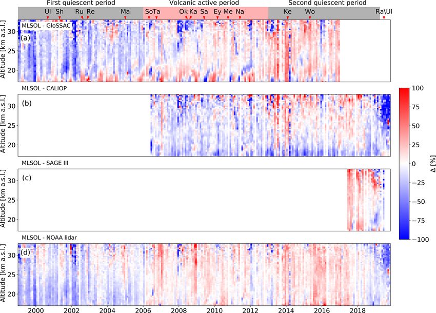
6824                             F. Chouza et al.: Long-term variability of stratospheric aerosol over Mauna Loa, Hawaii

and the scattering ratio approach. Generally speaking, these      Rayleigh extinction is applied to the Rayleigh and Raman
methods require the knowledge of a reference atmospheric          channel signals to be used in the calculation of the scattering
density profile, which is usually derived from co-located ra-     ratio (Eqs. 1 and 2):
diosonde launches or atmospheric models. In the case of ML-
SOL, and because this system has Rayleigh and nitrogen Ra-                     N355,corr (z)
                                                                  P355 (z) =     2
                                                                                             ,                                (1)
man channels with high enough signal-to-noise ratio (SNR)                       Tm,355 (z)
to cover the stratospheric aerosol layer, the scattering ratio                    N387,corr (z)
approach is used, which can be determined based on the ra-        P387 (z) =                        ,                         (2)
                                                                               Tm,355 (z)Tm,387 (z)
tio of the Rayleigh and Raman signals according to the pro-
cedure described elsewhere (Gross et al., 1995; Langenbach        where Pλ (z) is the Rayleigh-extinction-corrected lidar sig-
et al., 2019).                                                    nal, Nλ,corr (z) is the saturation and background-corrected li-
   The main advantage of using the Raman channel as               dar signal, and Tm,λ (z) is the one-way Rayleigh atmospheric
the atmospheric density reference profile for MLSOL is            transmission for λ = 355 and 387 nm. The extinction pro-
the smaller sensitivity to timing uncertainty. Since before       files required for this correction are derived from the closest
April 2019 the data acquisition of MLSOL had a range reso-        pressure and temperature profiles available from MERRA-
lution of 300 m, the determination of the range zero bin with     2. While the effect of the aerosol extinction could also be
an accuracy better than 150 m could not be done with the tra-     included in the calculation or corrected using an iterative ap-
ditional approach of looking for the first bin with nonzero       proach (Friberg et al., 2018), its contribution is small for the
readings. An error of 150 m (half a bin in the old MLSOL          cases presented in this study and compared to other uncer-
configuration) in the assumption of the range zero bin can in-    tainty sources.
troduce errors of up to 100 % in the calculation of the aerosol      The normalization is performed by dividing the signals by
backscatter coefficient (βa ) and aerosol optical depth (AOD)     the average of the Rayleigh (P355 (zref )) and Raman signals
in the stratosphere if the Klett method is used. This is mainly   (P387 (zref )) at a reference altitude range assumed to be free
due to the error introduced at the time of the so-called range    of aerosols (zref = 35–37 km a.s.l. in this study).
correction. Although alternative methods can be applied to
determine sub-bin timing in coarse-resolution systems, this                 P355 (z)P387 (zref )
is only possible if access to the configuration under study is    SR(z) =                                                     (3)
possible. Since several changes have been introduced in the                 P387 (z)P355 (zref )
systems over the last 20 years, an accurate timing charac-        The scattering ratio is finally calculated as the ratio of
terization of old setups is not possible. In contrast, the use    the normalized and corrected Rayleigh and Raman signals
of the ratio of the Rayleigh and Raman channels cancel the        (Eq. 3).
effect of the quadratic range dependence that characterizes li-
dar signals without the need to know the range zero bin. The      βa (z) = (SR(z) − 1)βm (z)                                  (4)
only requirement is a well-known relative timing difference
between the two channels. Since the Rayleigh and Raman            Once the scattering ratio is calculated, the aerosol backscatter
backscatter share the same laser and acquisition timing, this     coefficient (βa (z)) can be retrieved if a molecular backscatter
difference is typically very close to zero. As a downside, and    profile (βm (z)) is assumed (Eq. 4). This reference profile can
due to the limited SNR of the Raman channel, the retrieved        be derived, as in the case of the molecular extinction, from
profiles are generally noisier than the ones obtained by the      the MERRA-2 dataset. Uncertainty is calculated following
Klett algorithm.                                                  the procedures detailed in Russell et al. (1979).
   The SR retrieval from MLSOL measurements starts with              In the case of the NOAA lidar, the Klett inversion approach
the calculation of the average of the recorded signals for        is followed, and the SR is calculated based on a radiosonde
each channel during the length of the measurement period.         and model-derived atmospheric density reference profile in-
Typical measurement periods for this lidar correspond to 2 h      stead of using a Raman channel. The normalization altitude
measurements after astronomical twilight. After an average        used is nearly always 38–40 km a.s.l., which has improved
profile is obtained for each channel, a correction of the lidar   the consistency when compared to the earlier archived pro-
signals for count pile-up (saturation) is applied. This is per-   files in the NDACC database.
formed by assuming a non-paralyzable model and dead times
that are derived based on the comparison between high- and        3.2   Extinction coefficient, lidar ratio, and AOD
low-intensity channels available on each system. Following
this, the signal background corresponding to moonlight, air-      While the Raman channel of MLSOL allows the independent
glow, and electronic noise is calculated as the mean of the       retrieval of the aerosol extinction coefficient profiles and li-
high-altitude tail of the recorded signals, where no contri-      dar ratio at 355 nm based on technique presented in Ansmann
bution of the laser scattering is expected. This background       et al. (1990), the application of this method for stratospheric
is then subtracted from each signal. Finally, a correction for    retrievals has been limited to relatively thick stratospheric

Atmos. Chem. Phys., 20, 6821–6839, 2020                                               https://doi.org/10.5194/acp-20-6821-2020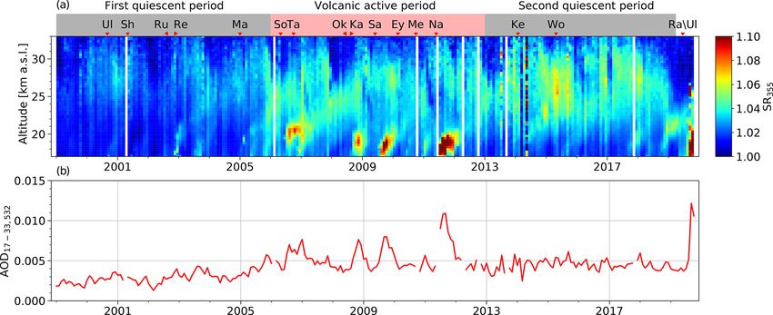
F. Chouza et al.: Long-term variability of stratospheric aerosol over Mauna Loa, Hawaii 6825
plume due to SNR constraints. As in the case of the backscat- Russia, a quiescent period between 1999 and 2006 was re-
ter coefficient retrieval, the molecular reference profile re- ported (Zuev et al., 2017). While all definitions imply some
quired for the inversion is obtained from MERRA-2 temper- degree of arbitrariness, the separation of the time series in
ature and pressure profiles. Based on balloon-borne measure- periods based on the intensity of the volcanic activity im-
ments (Jäger and Deshler, 2002), the extinction Ångström pact helps to organize the discussion. In the case of the ML-
exponent relating the Rayleigh and Raman wavelengths is SOL data series, corresponding to a tropical station, a similar
assumed to be −1.6. Once a stratospheric extinction profile background period between January 1999 and January 2006
is derived, the lidar ratio of the stratospheric plume under can be defined. Although a few eruptions took place during
study is calculated as the ratio of the extinction and backscat- that time frame, with some occurring at equatorial latitudes,
ter profiles. In this work, the Raman technique is applied to no strong impact in the total stratospheric AOD was observed
measurements conducted on the Nabro plume, and the results by MLSOL.
are compared to similar previous measurements (Sect. 5). The first two eruptions that occurred during this period,
Unfortunately, because the Raman-based extinction coef- corresponding to the Ulawun and Shiveluch volcanos, did
ficient retrieval approach is not able to provide acceptable not show a clear impact in the extinction profiles derived
results during most of the period under study because of the from MLSOL. After October 2002, some plumes, presum-
generally low aerosol load conditions, the extinction coeffi- ably corresponding to the Ruang and Reventador eruptions,
cient profiles presented in Sects. 4 and 6 are based on the were observed as covering a relatively short period of time
assumption of a constant lidar ratio. Since the satellite-borne with a small impact on the stratospheric AOD. During the
datasets provide extinction profiles at either 525 or 532 nm, background period defined for the MLSOL station, the lidar-
the MLSOL backscatter measurements are first translated to derived AOD is (2.9 × 10⁻³ ± 0.1 × 10⁻³ ). The variability
532 nm using the backscatter coefficient color ratio derived reported corresponds to 1σ .
from co-located NOAA lidar measurements (Sect. 5.1). Fol-
lowing this, NOAA lidar and MLSOL backscatter profiles 4.2 The volcanic active period (2006–2013)
are converted to extinction profiles by assuming a lidar ratio
of 50 sr, as typically referenced in previous studies (Trickl During the time period comprehended between January 2006
et al., 2013; Khaykin et al., 2017). and January 2013, several volcanic eruptions with VEI ≥ 4
Finally, the stratospheric AOD is calculated by integrating took place in the tropics and Northern Hemisphere. The sig-
the extinction coefficient profiles between 17 and 33 km. natures of most of these eruptions are clearly visible in the
The calculation of the extinction coefficient uncertainty is scattering ratio profiles presented in Fig. 1. These signa-
performed based on a Monte Carlo analysis, adopting a 3 % tures are characterized by a steep increase in the AOD as
standard deviation as the uncertainty on the temperature and the plume reaches the MLSOL station, followed by an AOD
pressure profiles from MERRA-2. decay over a period of several months. The e-folding de-
cay time for the AOD eruption signatures that occurred in
this period is between 3 and 5 months, with a peak AOD of
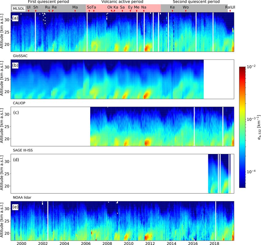
4 The JPL Mauna Loa historical record (1999–2019) 11×10−3 registered in August 2011 as the result of the Nabro
eruption (Sawamura et al., 2012). Between eruptions, the
Between 1 January 1999 and 1 November 2019, MLSOL AOD quasi-background level reported by MLSOL is about
conducted 2732 measurement sessions with an average du- (5 × 10⁻³ ± 0.4 × 10⁻³ ), almost 70 % higher than during the
ration of 2 h. Based on the method presented in the previ- quiescent period described in the previous section.
ous section (Sect. 3), scattering ratio profiles at 355 nm and Despite the fact that stratospheric aerosols interact with in-
stratospheric AOD values at 532 nm were retrieved and av- coming solar radiation and stratospheric chemistry and are
eraged to provide a monthly mean time series (Fig. 1). The subject to evaporation and sedimentation (Kremser et al.,
number of profiles included in the monthly mean calcula- 2016), they proved to be a useful quasi-passive trace to inves-
tion change over time depending on the number of available tigate stratospheric circulation (Trepte et al., 1993). In partic-
measurements, with a minimum of 1, a maximum of 41, and ular, the diabatic plume ascent induced by residual Brewer–
a mean of 11. Due to technical issues, measurements con- Dobson circulation (BDC) has been studied based on several
ducted between the start of the operations in 1994 and the satellite observations (Trepte and Hitchman, 1992; Vernier
end of 1998 are not included in the discussion. et al., 2009; Fairlie et al., 2014). While analyzing the vertical
evolution of the volcanic plumes shown in Fig. 1, a typical
4.1 The first “quiescent” period (1999–2006) “tape-recorder-like” signature as in the case of water vapor
observations (Mote et al., 1996) can be seen. Over the life-
Several studies focusing on midlatitudes refer to the time pe- time of the eruption plumes, the bottom and top of the plume
riod between 1997 and 2003 as a quiescent or background elevate at a similar rate. In some cases, as previously reported
period (Trickl et al., 2013; Sakai et al., 2016; Khaykin et al., by Vernier et al. (2011), the space left by the plumes is filled
2017). In the case of the midlatitude station located in Tomsk, with overshooting tropospheric clean air.
https://doi.org/10.5194/acp-20-6821-2020 Atmos. Chem. Phys., 20, 6821–6839, 2020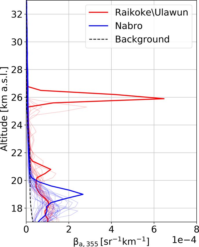
6826                                F. Chouza et al.: Long-term variability of stratospheric aerosol over Mauna Loa, Hawaii

Figure 1. Monthly averaged time series of the stratospheric scattering ratio at 355 nm retrieved from MLSOL between January 1999 and
November 2019 (a). Eruptions with a VEI ≥ 4 that occurred during this period are indicated at the top of the plot (see Table 1). Three
different periods defined based on the impact of the volcanic activity are also shown (see text for details). Monthly averaged AOD retrieved
from MLSOL extinction profiles (b).

Table 1. List of eruptions with VEI ≥ 4 in the tropics and Northern Hemisphere between January 1999 and November 2019. Information
regarding the location of the erupting volcano and the maximum plume altitude (MPA) reported by the Global Volcanism Program is included
for reference (https://volcano.si.edu/, last access: 10 May 2020). The Raikoke eruption is included in the list, although the VEI has not been
determined yet. NA – not available.

                             Volcano                 Eruption date    Location                        MPA (km)
                             Ulawun (Ul)             Sep 2000         Papua New Guinea (5.0◦ S)       16
                             Shiveluch (Sh)          May 2001         Kamchatka (56.6◦ N)             NA
                             Ruang (Ru)              Sep 2002         Indonesia (2.3◦ N)              22
                             Reventador (Re)         Nov 2002         Ecuador (0.0 ◦ N)               17
                             Manam (Ma)              Jan 2005         Papua New Guinea (4.1◦ S)       24
                             Soufrière Hills (So)    May 2006         West Indies (16.7◦ N)           20
                             Tavurvur (Ta)           Oct 2006         Papua New Guinea (4.2◦ S)       18
                             Okmok (Ok)              Jul 2008         Aleutian Islands (53.46◦ N)     15
                             Kasatochi (Ka)          Aug 2008         Aleutian Islands (52.17◦ N)     15
                             Sarychev (Sa)           Jun 2009         Kuril Islands (48.1◦ N)         17
                             Eyjafjallajökull (Ey)   Mar 2010         Iceland (63.6◦ N)               9
                             Merapi (Me)             Oct 2010         Indonesia (7.5◦ S)              17
                             Nabro (Na)              Jun 2011         Eritrea (13.4◦ N)               18
                             Kelud (Ke)              Feb 2014         Indonesia (7.9◦ S)              19
                             Wolf (Wo)               May 2015         Galápagos Islands (0.0◦ N)      7
                             Ulawun (Ul)             Jun 2019         Papua New Guinea (5.0◦ S)       NA
                             Raikoke (Ra)            Jun 2019         Sea of Okhotsk (48.3◦ N)        17

   By analyzing the aerosol plume height evolution over                  to estimate the plume center. The result of this calculation,
time, a rough estimation of the apparent BDC ascent rate can             shown as black crosses in Fig. 2, allow us to estimate the as-
be calculated. Figure 2 presents a close-up of the MLSOL                 cent rate between 18 and 19 km a.s.l. to be about 0.6 km per
measurements of the Sarychev plume and the altitude evo-                 month (0.025 cm s−1 ). As the plume rises further, the ascent
lution of the center of the plume as a function of time. For             speed seems to diminish, but a quantitative estimation based
the calculation of the center of the plume, the background               on MLSOL data is difficult due to the reduced SNR. This
extinction calculated based on the mean extinction of the                result is on the same order of magnitude as those retrieved
6 months prior to the eruption is first subtracted from the              based on water vapor and carbon monoxide tape recorder sig-
extinction time series. Since the plume has a vertical profile           natures (Minschwaner et al., 2016) and double the ascent rate
shape similar to a Gaussian function, a function fit is used             derived from CALIOP measurements of the Soufrière Hills

Atmos. Chem. Phys., 20, 6821–6839, 2020                                                     https://doi.org/10.5194/acp-20-6821-2020
F. Chouza et al.: Long-term variability of stratospheric aerosol over Mauna Loa, Hawaii                                            6827

Figure 2. Monthly stratospheric aerosol backscatter corresponding
to the Sarychev eruption plume derived from MLSOL. The center
of the plume for each month is also shown (crosses, black).

plume (Vernier et al., 2011). For the period between the end
of 2009 and beginning of 2010, the ascent rate derived from
water vapor records was estimated to be about 0.02 cm s−1 at
51 hPa (about 19 km a.s.l.).
                                                                    Figure 3. Nighttime CALIOP tracks (dashed black) in the MLO
4.3   The second quiescent period (2013–2019) and                   (red cross) area analyzed as part of the PyroCb plume tracking. The
      Raikoke eruption                                              spatial extension of the stratospheric aerosol plumes detected during
                                                                    the overpasses are highlighted with thick black lines. MERRA-2
After the decay of the Nabro eruption plume and before the          winds at 100 hPa are also shown (black arrows).
Raikoke eruption, a second relatively quiescent period can
be defined based on the aerosol extinction coefficient and
AOD records. Although during this period, defined between           by the MERRA-2 reanalysis. Additionally, compatible re-
early 2013 and July 2019, some eruptions with VEI ≥ 4 oc-           sults can be seen in Fig. 3c presented in Kloss et al. (2019),
curred, only a slight impact was observed on both the ex-           where transport simulations of the British Columbia fire’s
tinction and AOD records. The observed mean AOD for the             smoke by the Chemical Lagrangian Model of the Strato-
period is 4.4 × 10⁻³ ± 0.7 × 10⁻⁴ , which is 50 % higher than       sphere (CLaMS) showed the presence of fire tracers over
that measured during the first quiescent period and similar to      Hawaii as early as 5 September 2017.
the AOD observed in the period measured between volcanic               Among these three CALIOP overpasses, the one corre-
eruptions in the volcanic active period.                            sponding to 31 August 2017 provides the closest temporal
   In addition to volcanic eruptions, large wildfires can also      and spatial data to what is believed to be the first observa-
contribute to an enhancement of the stratospheric aerosol           tion of stratospheric smoke injected by the British Columbia
load (e.g., Khaykin et al., 2018; Zuev et al., 2019). On            fires at MLO. An overview of the CALIOP total attenuated
12 August 2017, five near-simultaneous extreme pyrocumu-            backscatter measurement during that overpass together with
lonimbus (PyroCb) events took place in British Columbia,            the MLSOL measurements for 1 September 2017 is pre-
Canada. According to recent studies (Peterson et al., 2018),        sented in Fig. 4.
these events injected a mass comparable to a midsized vol-             Although the plume visible in CALIOP L1 profiles
canic eruption into the stratosphere. In the case of MLSOL,         (Fig. 4b) does not seem to reach the MLO latitude, this could
the smoke plume corresponding to the British Columbia               be attributed to several reasons, including the lower sensi-
fires was first sensed on 1 September 2017 as a very de-            tivity of CALIOP when compared to MLSOL and the spa-
fined layer of about 1.5 km thickness at 16 km a.s.l. In or-        tiotemporal difference between measurements. In order to
der to relate the origin of this plume to the British Columbia      provide a quantitative assessment of the plume character-
fires and minimize the possibility of a cirrus cloud misclas-       istics observed by CALIOP on 31 August 2017 and com-
sification, three nighttime CALIOP overpasses around the            pare it with the MLSOL observations during 1 Septem-
Mauna Loa Observatory (MLO) area between 29 August                  ber 2017, an aerosol backscatter profile was derived from
and 2 September 2017 were analyzed. For all these over-             the CALIOP L1 total attenuated backscatter averaged over
passes, a thin stratospheric plume at about 15 km a.s.l. was        the southern end of the plume (21 to 22◦ N). This conver-
observed 150 km north of MLO (Fig. 3). In all cases, the            sion includes the correction for molecular and ozone extinc-
plumes were characterized by a low average particle depo-           tion and the subtraction of the molecular backscatter com-
larization ratio (< 0.1), which is compatible with smoke par-       ponent calculated from co-located MERRA-2 temperature
ticles (Kim et al., 2018). The rapid equatorward transport of       and pressure profiles. The intercomparison (Fig. 4a) reveals
the plume seems in agreement with the wind field reported           a strong similarity between the plume elevation and thick-

https://doi.org/10.5194/acp-20-6821-2020                                              Atmos. Chem. Phys., 20, 6821–6839, 2020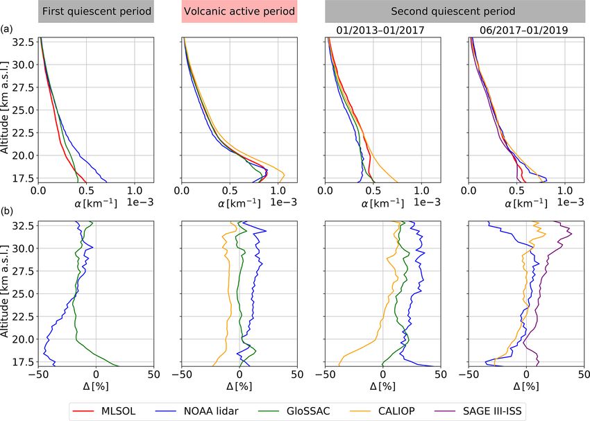
6828 F. Chouza et al.: Long-term variability of stratospheric aerosol over Mauna Loa, Hawaii
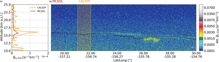
Figure 4. Overview of the CALIOP attenuated backscatter measurements during the 31 August 2019 overpass in the Hawaii area (a). The
1 September 2019 MLSOL aerosol backscatter observations (b, red) are presented together with the aerosol backscatter retrieval from the
CALIOP (a, orange) for the southern part of the plume (shaded orange).
ness measured by CALIOP and MLSOL. On the other side,
the backscatter coefficient derived from CALIOP measure-
ments peaks at about 1.5 × 10⁻⁴ sr−1 km−1 , while the ML-
SOL measurement on 1 September 2017 has a peak value
of about 0.2 × 10⁻⁴ sr−1 km−1 . In both cases, the backscat-
ter is reported at 532 nm. The MLSOL aerosol backscatter
was converted to 532 nm using a color ratio of 0.8 as de-
rived in Sect. 5.1 from co-located MLSOL and NOAA lidar
measurements. After the first detection on 1 September 2017,
several other plumes were observed by MLSOL over a pe-
riod of 5 months, with a maximum average plume center al-
titude of 19.5 km a.s.l. registered during February 2018 (not
shown). While at midlatitudes this PyroCb event produced
a large enhancement of the stratospheric AOD (Baars et al.,
2019), with peak values over 0.2, only slight AOD variations
were observed at Mauna Loa.
The Raikoke and Ulawun volcanic eruptions, occurring on
22 and 26 June 2019, put an end to the second stratospheric Figure 5. MLSOL-derived daily extinction coefficient profiles for
“quiescent” period at Mauna Loa. Although the VEIs of these September and October 2019 (solid light red). The extinction co-
eruptions are still not quantified, the monthly averaged strato- efficient profile for 24 September 2019 is highlighted (solid red).
spheric AOD derived from MLSOL for September 2019 was For comparison, the MLSOL-derived daily profiles of the Nabro
0.012, the highest measured value over the last 20 years. plume between the end of July 2011 and January 2012 are presented
In contrast to previous observations of eruption plumes at (solid light blue), with the most prominent profile highlighted (solid
Mauna Loa, which mainly remained confined to altitudes be- blue). As background aerosol reference, the monthly averaged ex-
tinction profile for June 2019 (black dashed) before the detection of
low 20 km a.s.l., a thick plume traced back to the Raikoke
the Raikoke–Ulawun plume is also shown.
eruption was observed at altitudes exceeding 26 km a.s.l. be-
tween the end of September and beginning of October 2019
(Fig. 5).
CALIOP L1 profiles considering the main stratospheric cir-
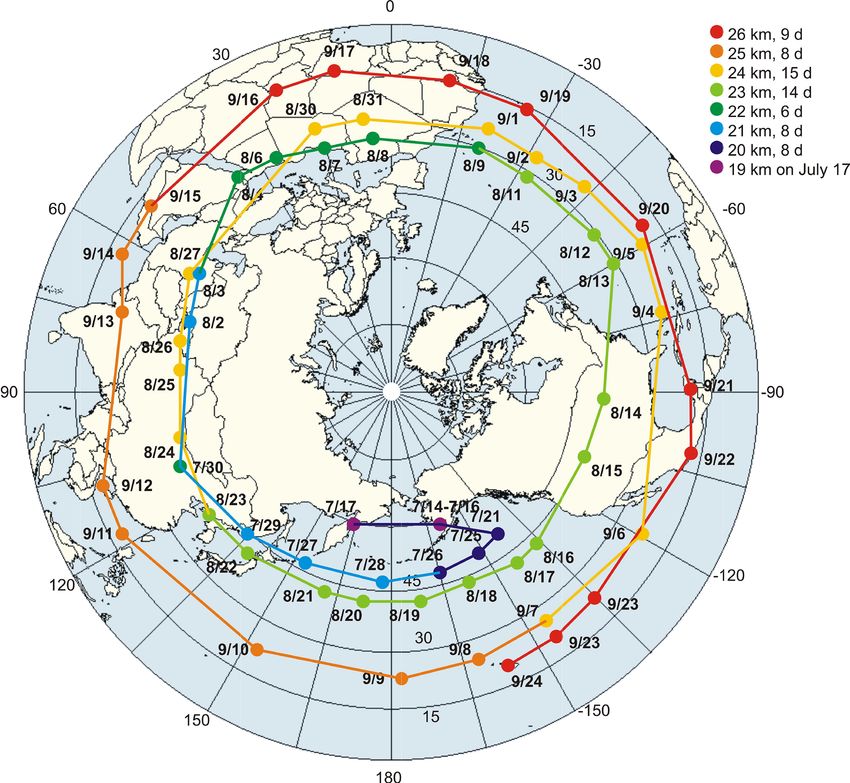
The back trajectory of the Raikoke plume observed at the
culation patterns. This was possible due to the well-defined
end of September 2019 by MLSOL was estimated based
shape of the plume and its strong backscattering proper-
on CALIOP L1 attenuated backscatter profiles (Fig. 6). The
ties when compared to other previously observed volcanic
tracking of this plume started with its first detection at Mauna
plumes.
Loa on 24 September 2019 and ended on 17 July 2019 over
While this well-defined and elevated plume is the most
the Kamchatka Peninsula, Russia. At that point, the track
prominent feature observed by MLSOL during the period
is lost as there are many different plumes in the region.
between July and November 2019, an enhancement of the
Over a period of slightly over 2 months, the plume ascended
aerosol load between the tropopause and 21 km a.s.l. was also
7 km, from 19 to 26 km a.s.l. The tracking of the plume was
observed during this period. In order to further investigate
conducted mainly through a manual inspection process of
whether this plume corresponded to the Raikoke eruption or
Atmos. Chem. Phys., 20, 6821–6839, 2020 https://doi.org/10.5194/acp-20-6821-2020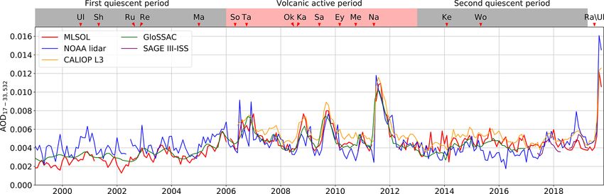
F. Chouza et al.: Long-term variability of stratospheric aerosol over Mauna Loa, Hawaii                                      6829

Figure 6. Back trajectory of the Raikoke plume between 24 September and 17 July 2019 derived from CALIOP L1 attenuated backscatter
profiles.

the Ulawun eruption, CALIOP L3 longitudinally averaged             5     Lidar-derived optical properties
SR cross sections (latitude vs. altitude) from this period are
presented in Fig. 7.                                               Most lidar-derived stratospheric aerosol long-term records
   Since no significant stratospheric injection events were        consist of backscatter coefficient profiles reported at 532 nm.
registered during the first half of 2019, the SR cross section     While some satellite-based datasets, like CALIOP, operate
from June 2019 can be considered the background condition          at the same wavelength and also provide aerosol backscat-
for this analysis (Fig. 7, BKG). Starting in July 2019, an en-     ter coefficient as its natural product, other instruments like
hancement of the aerosol load is clearly visible between the       those of the SAGE series provide extinction profiles at other
tropopause and 19 km a.s.l., with a small gap around 15◦ N.        wavelengths (e.g., 525 nm). In the latter case, the compar-
This gap corresponds to the division between the plume of          isons with ground-based lidar datasets require knowledge of
the Ulawun (south) and Raikoke (north) eruptions. By Au-           the lidar ratio, which is typically derived using Raman lidar
gust 2019, this gap is closed as both plumes mixed together,       measurements. On the other hand, the recently launched Ae-
making them indistinguishable. Between 30 and 40◦ N, a             olus wind lidar mission (Stoffelen et al., 2005; Flamant et al.,
fraction of the Raikoke plume is visible rising above the          2008) will provide aerosol backscatter and extinction profiles
rest of the plume, confirming the back trajectories presented      in the lowermost stratosphere at 355 nm. Its validation and
in Fig. 6. By September 2019, the mixed Ulawun–Raikoke             intercomparison with other datasets (like CALIOP) will then
plume reaches 21 km a.s.l. and increases its SR at low lat-        require a good knowledge of the backscatter and extinction
itudes. The secondary Raikoke plume displaces southward,           wavelength dependence.
reaching 20◦ N at an altitude of over 25 km a.s.l. Finally, the
October 2019 cross section starts to show a decay in the SR        5.1    The color ratio of the backscatter coefficient
of the plume, which is compatible with the AOD measure-
ments by MLSOL recorded for that month (Fig. 1).                   Based on the co-located backscatter coefficient profiles of
                                                                   MLSOL, NOAA lidar, and CALIOP, the backscatter color
                                                                   ratio (and backscatter Ångström exponent) between 355 and

https://doi.org/10.5194/acp-20-6821-2020                                            Atmos. Chem. Phys., 20, 6821–6839, 2020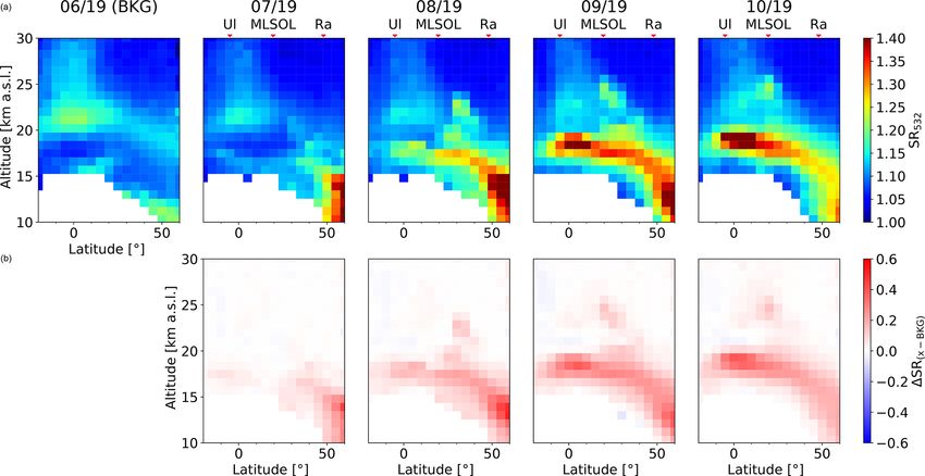
6830                             F. Chouza et al.: Long-term variability of stratospheric aerosol over Mauna Loa, Hawaii

Figure 7. Longitudinally averaged CALIOP L3 SR cross sections (latitude–height) between June and October 2019 (a) are shown together
with their difference (b) with respect to the background conditions presented during June 2019.

532 nm was calculated as function of altitude and time. Fig-        the eruptions only affected the lower part of the SAL. When
ure 8 presents the temporal average of the color ratio for the      analyzing the results below 20 km a.s.l., the color ratio de-
volcanic and second quiescent period. In the case of the color      rived from the CALIOP–MLSOL data pair show values that
ratio derived from CALIOP and MLSOL measurements, the               rise up to about 0.7 in the volcanic active period and 0.8 in
monthly means from both datasets are used. In the case of the       the quiescent period, while the NOAA lidar–MLSOL pair
color ratio derived from the two ground-based lidars, only          show a fairly constant color ratio of about 0.5. This discrep-
same-day measurements are included in the calculation. Be-          ancy is going to be further discussed in the following section
cause measurements from CALIOP are available only during            (Sect. 6).
the volcanic active period and second quiescent period, the            Throughout this work, when the backscatter coefficient de-
measurements from NOAA lidar during the first quiescent             rived from MLSOL measurements at 355 nm is required to be
period are excluded to simplify the comparison.                     converted to 532 nm (e.g., Sect. 3.2), a smoothed version of
   Generally speaking, a large color ratio (close to unity) in-     the average of the two color ratio profiles derived from the
dicates the presence of large particles and is directly asso-       NOAA lidar and MLSOL measurements is used. The val-
ciated with a small Ångström exponent (Jäger and Deshler,           ues, about 0.5, are in reasonable agreement with the ones re-
2002). This was well documented during the Pinatubo erup-           ported by Jäger and Deshler (2002) at the end period affected
tion, when Ångström exponent values derived from balloon-           by the Pinatubo eruption, with a backscatter Ångström expo-
borne measurements were very close to zero during the first         nent equal to −1.4, corresponding to a color ratio between
months after the eruption and slowly increased as the plume         532 and 355 nm of 0.57.
dissipated (Jäger and Deshler, 2002). In this case, because            In the case of high-aerosol events, the color ratio of spe-
the eruptions occurred during the volcanic active period were       cific plumes can be derived based on the simultaneous mea-
relatively small, no large variations in the color ratio are ex-    surements of NOAA lidar and MLSOL. Figure 9 presents
pected between the two defined periods. In fact, the color          two examples, one corresponding to the plume of the Nabro
ratio profiles derived from the three lidar datasets show sim-      eruption and a second example corresponding to the British
ilar results above 20 km a.s.l., with values close to 0.5 and       Columbia smoke plume. In both cases, the plumes show
a slight increase as we go from the top of the SAL to about         higher color ratios than the surrounding. In the case of the
20 km a.s.l. One exception is the case of the CALIOP-derived        Nabro example, the average color ratio above the plume is
color ratio during the volcanic active period, where results        approximately 0.4, while in the plume the average is about
are about 20 % higher than for the rest of the cases. This          0.5. The values observed above the plume are also below the
result is unexpected, as it does not show a good agreement          average for other cases (not shown). For the PyroCb plume,
with the other datasets and periods, considering that most of       the color ratio has a peak value of about 0.8 (correspond-

Atmos. Chem. Phys., 20, 6821–6839, 2020                                               https://doi.org/10.5194/acp-20-6821-2020
F. Chouza et al.: Long-term variability of stratospheric aerosol over Mauna Loa, Hawaii                                          6831

                                                                        l’Analisi Ambientale (CNR-IMAA) of the Nabro plume lidar
                                                                        ratio at 355 nm was reported to be (55 ± 18) sr by Sawamura
                                                                        et al. (2012). Considering the large uncertainties associated
                                                                        with these measurements and the spatiotemporal difference
                                                                        in the plume sampling, the results can be considered to be in
                                                                        reasonable agreement.

                                                                        6   Intercomparison between MLSOL, NOAA lidar, and
                                                                            satellite-based datasets

                                                                        The retrieval of the extinction coefficient out of the CALIOP
                                                                        measurements requires the assumption of a lidar ratio. In the
                                                                        case of the fraction of the GloSSAC dataset where CALIOP
                                                                        is included, this is assumed to be 53 sr, while in the CALIOP
                                                                        L3 data product and the profiles derived from MLSOL and
                                                                        NOAA lidar, a lidar ratio of 50 sr is used.
                                                                           Another point to take into account while comparing the
                                                                        datasets is the differences in their spatial resolution. The
                                                                        GloSSAC dataset provides a zonal average of the extinction
                                                                        profile for a latitude bin of 5◦ . In contrast, the CALIOP L3
Figure 8. Average color ratio for the volcanic (solid red) and second   dataset has a longitudinal resolution of 20◦ . In the case of
quiescent (solid black) periods derived from CALIOP and MLSOL
                                                                        MLSOL and NOAA lidar and given their ground-based na-
measurements (a) and NOAA lidar and MLSOL measurements (b).
The 1σ variability is indicated by the shaded areas.
                                                                        ture and uneven temporal sampling, extinction profiles cor-
                                                                        respond to a very small atmospheric volume, making them
                                                                        more susceptible to small-scale variability. With regard to the
ing to an Ångström exponent of −0.6), and values above the              vertical resolution and in order to calculate the correspond-
plume are in good agreement with the mean corresponding                 ing AOD, an interpolation of the GloSSAC and CALIOP L3
to the second quiescent period.                                         datasets needs to be introduced in order to match the MLSOL
                                                                        and NOAA lidar grids.
5.2   Lidar ratio of stratospheric volcanic aerosols                       Finally, it is important to notice that the backscatter re-
      measured after Nabro eruption (2011)                              trievals from MLSOL are performed at 355 nm. In order to
                                                                        compare them with the GloSSAC, CALIOP, and NOAA li-
Due to SNR limitations, direct measurements of strato-                  dar datasets, a conversion following the results from Sect. 5.1
spheric aerosol extinction profiles by Raman lidars are not             is applied. For the conversion of the GloSSAC extinction
common and typically restricted to strong volcanic events               dataset from 525 to 532 nm, a constant Ångström exponent
like the 1991 Mt. Pinatubo (Ferrare et al., 1992; Ansmann               of −1.6 is used (Jäger and Deshler, 2002).
et al., 1993), 2009 Sarychev Peak (Mattis et al., 2010), and               The extinction coefficient time series for the five datasets
2011 Nabro eruptions (Sawamura et al., 2012). For this rea-             under consideration are presented in Fig. 11. As can be seen
son, most of the long-term stratospheric aerosol lidar studies          here, there is a general qualitative agreement between all the
rely on a lidar ratio derived out of balloon-borne in situ mea-         datasets. In the case of GloSSAC and CALIOP, due to the
surements (Jäger et al., 1995). In this study, and thanks to            higher amount of more evenly distributed measurements in-
the large receiver, laser power, and elevation of MLSOL, di-            cluded in the time series calculation, a smoother time series
rect aerosol extinction measurements during the Nabro erup-             can be observed. In the case of GloSSAC, slight discontinu-
tion are presented. These measurements allow, in combina-               ities in the extinction time series can be noticed around 2006
tion with the derived backscatter profiles, the retrieval of the        and 2007, which is likely to be caused by changes in the in-
lidar ratio associated with the volcanic plume.                         struments used for the retrieval as described in Sect. 2.
   The results presented in Fig. 10, correspond to measure-                At the bottom of the stratospheric aerosol layer, between
ments conducted on 19 July 2011 by MLSOL. A well-                       17 and 23 km a.s.l., aerosol plumes corresponding to differ-
defined plume with a peak backscatter coefficient of 0.75 ×             ent stratospheric injection events are clearly visible in all
10−3 sr−1 km−1 was found at 18.7 km. The corresponding                  datasets. The largest contributions can be easily correlated
extinction was measured to be 4.8 × 10⁻² km−1 , leading to              to volcanic eruptions that occurred in the Northern Hemi-
a lidar ratio of (64 ± 12.7) sr at 355 nm around the cen-               sphere (Table 1) during the period under study. Due to the
ter of the plume. The measurement conducted by the Con-                 strong zonal winds in the lower stratosphere, the MLSOL,
siglio Nazionale delle Ricerche - Istituto di Metodologie per           NOAA lidar, and CALIOP datasets do not show large dif-

https://doi.org/10.5194/acp-20-6821-2020                                                 Atmos. Chem. Phys., 20, 6821–6839, 2020
6832 F. Chouza et al.: Long-term variability of stratospheric aerosol over Mauna Loa, Hawaii Figure 9. Backscatter derived from MLSOL (red) and NOAA lidar (blue) and corresponding color ratios for the Nabro plume (a, b) and the British Columbia (pyroCb) smoke plume (c, d). In the color ratio plots, the corresponding average color ratio derived for the volcanic active and second quiescent period (see Fig. 8b) is included for reference (dashed black). The altitude interval affected by these two features is highlighted in grey. Figure 10. Backscatter (a) and extinction coefficient (b) profiles at 355 nm measured by MLSOL on 19 July 2011. The derived lidar ratio is also shown (c). ferences with respect to the zonally averaged GloSSAC and ing the volcanic active period and most of the second qui- SAGE III-ISS datasets. The top of the layer, on the other escent period. After the second half of 2018, slightly higher hand, shows a modulation on its top altitude that can be as- values are reported by NOAA lidar. For the difference be- sociated with the quasi-biannual oscillation (Hommel et al., tween MLSOL and GloSSAC (Fig. 12a), a similar tempo- 2015). In this case, the maximum of the SAL was observed rally dependent variation is observed, with GloSSAC show- to be at about 32 km a.s.l., while its minimum can reach as ing higher extinction values during the first quiescent period low as 26 km a.s.l. and lower values than MLSOL during the volcanic active and In order to provide a better overview of the differences be- second quiescent periods. Below 20 km a.s.l., the effect of tween the datasets under study, the mean relative differences the zonal average on the GloSSAC dataset can be appreci- between MLSOL and the other four datasets as a function of ated during volcanic injection events. The zonal average in- altitude and time are presented in Fig. 12. The difference be- troduces a small shift in the plume temporal shape, which in tween the two ground-based lidars (Fig. 12d) shows a slight turn translates into higher values reported by GloSSAC fol- temporally dependent extinction coefficient difference with lowed by higher values reported by MLSOL. While compar- higher values reported by NOAA lidar during the first qui- ing MLSOL with the CALIOP L3 dataset (Fig. 12b), higher escent period, and higher values reported by MLSOL dur- extinction values are generally shown by CALIOP L3. This Atmos. Chem. Phys., 20, 6821–6839, 2020 https://doi.org/10.5194/acp-20-6821-2020
F. Chouza et al.: Long-term variability of stratospheric aerosol over Mauna Loa, Hawaii                                           6833

Figure 11. Intercomparison between the monthly mean stratospheric extinction derived from MLSOL, GloSSAC, CALIOP, SAGE III, and
NOAA lidar. (a) Extinction coefficient derived from MLSOL measurements between January 1999 and November 2019. (b) Extinction co-
efficient from the GloSSAC dataset between January 1999 and December 2016. (c) Extinction coefficient from CALIOP L3 dataset between
June 2006 and December 2018. (d) Extinction coefficient from SAGE III between June 2017 and April 2019. (e) Extinction coefficient de-
rived from NOAA lidar measurements between January 1999 and April 2019. Eruptions listed in Table 1 are indicated as small red triangles
on top of (a) together with the three time periods defined in Sect. 4.

is opposite to what GloSSAC shows for the same time period               Figure 13 provides a more quantitative analysis of the dif-
(for which CALIOP and OSIRIS measurements are used). In               ferences between datasets by averaging the results provided
order to discard the influence of the zonal averaging in GloS-        in Figs. 11 and 12 over the three periods under study (first
SAC, the CALIOP L3 datasets were zonally averaged. The                quiescent, volcanic active, and second quiescent periods). Al-
results (not shown) did not reveal a significant influence of         though the general agreement between datasets is good, with
the zonal average that can explain this difference. Finally, the      a maximum relative difference usually around 25 % above
difference with SAGE III-ISS (Fig. 12c) indicates generally           23 km, the differences tend to grow towards the bottom of the
higher extinction values by MLSOL, with a small change to-            vertical profiles. Although in the case of MLSOL and NOAA
wards the end of 2018 and beginning of 2019.                          lidar this difference likely originates from different retrieval
                                                                      approaches, including noise subtraction and normalization,

https://doi.org/10.5194/acp-20-6821-2020                                                Atmos. Chem. Phys., 20, 6821–6839, 2020
6834 F. Chouza et al.: Long-term variability of stratospheric aerosol over Mauna Loa, Hawaii
Figure 12. Mean relative difference between MLSOL and GloSSAC (a), CALIOP (b), SAGE
III (c), and
NOAA lidar (d). The mean relative
difference between MLSOL and each other dataset (X) is calculated as (MLSOL − X) / MLSOL+X
2 × 100 %.
systematic errors caused by misalignment cannot be ruled lower AOD values until 2006. After that, the tendency re-
out. The relative impact of these error sources is currently verts, with NOAA lidar-derived values generally slightly be-
under investigation. Other differences, as the one shown with low MLSOL. As expected from the differences presented in
the new CALIOP L3 data product, seem to be more sys- Figs. 12 and 13, the CALIOP-derived AOD is the one show-
tematic, with CALIOP exhibiting consistently higher extinc- ing the largest discrepancy with the other datasets, with val-
tion values when compared with the other two satellite-based ues consistently larger (between 12 % and 22 %) than the
datasets and MLSOL. When comparing with NOAA lidar, rest. For the period influenced by the Raikoke plume, and as
the CALIOP dataset also tends to show higher extinction val- in the case of MLSOL, the AOD derived from the NOAA
ues below 23 km, with the exception of the second half of the lidar also shows the highest value of the time series. For
second quiescent period, where the agreement is good. The September 2019, the mean AOD derived from MLSOL mea-
agreement of MLSOL with GloSSAC is good, with a relative surements was 0.012, while for the NOAA lidar it was 0.016.
difference consistently below 20 %. This difference likely originate from the difference in the
As a final metric to evaluate the agreement between number of measurements performed by both instruments. In
datasets, the corresponding stratospheric AOD at 532 nm the case of MLSOL, 16 measurements were conducted dur-
is calculated for the period comprehended between Jan- ing September 2019, while only 2 were performed by the
uary 1999 and November 2019 and presented in Fig. 14. NOAA lidar. A general metric of the agreement between
As expected from the differences observed between the ex- datasets is presented in Table 2, where the mean relative
tinction datasets, the MLSOL-derived AOD time series show differences between AOD time series (Xrow,column ) are pre-
slightly lower values than GloSSAC and NOAA lidar dur- sented.
ing the first half of the first quiescent period. After 2003,
the agreement between MLSOL and GloSSAC becomes very
good. When compared with NOAA lidar, MLSOL shows
Atmos. Chem. Phys., 20, 6821–6839, 2020 https://doi.org/10.5194/acp-20-6821-2020You can also read