Return Period of Characteristic Discharges From the Comparison Between Partial Duration and Annual Series, Application to the Walloon Rivers ...

Article
Return Period of Characteristic Discharges
From the Comparison Between Partial Duration
and Annual Series, Application to the Walloon Rivers
(Belgium)
Jean Van Campenhout *, Geoffrey Houbrechts, Alexandre Peeters and François Petit
 Hydrography and Fluvial Geomorphology, UR Spheres, Research Centre, Department of Geography,
 University of Liège, 4000 Sart‐Tilman, Liège, Belgium; g.houbrechts@uliege.be (G.H.);
 a.peeters@uliege.be (A.P.); francois.petit@uliege.be (F.P.)
 * Correspondence: jean.vancampenhout@uliege.be; Tel.: +32‐4‐366‐52‐97

 Received: 27 January 2020; Accepted: 8 March 2020; Published: 12 March 2020

 Abstract: The determination of the return period of frequent discharges requires the definition of
 flood peak thresholds. Unlike daily data, the volume of data to be processed with the
 generalization of hourly data loggers or even with an even finer temporal resolution quickly
 becomes too large to be managed by hand. We therefore propose an algorithm that automatically
 extracts flood characteristics to compute partial series return periods based on hourly series of flow
 rates. Thresholds are defined through robust analysis of field observation‐independent data to
 obtain five independent flood peaks per year in order to bypass the 1‐year limit of annual series.
 Peak over thresholds were analyzed using both Gumbel’s graphical method and his ordinary
 moments method. Hydrological analyses exhibit the value in the convergence point revealed by
 this dual method for floods with a recurrence interval around 5 years. Pebble‐bedded rivers on
 impervious substratum (Ardenne rivers) presented an average bankfull discharge return period of
 around 0.6 years. In the absence of field observation, the authors have defined the bankfull
 discharge as the Q0.625 computed with partial series. Annual series computations allow Q100
 discharge determination and extreme floods recurrence interval estimation. A comparison of data
 from the literature allowed for the confirmation of the value of Myer’s rating at 18, and this value
 was used to predict extreme floods based on the area of the watershed.

 Keywords: return period; bankfull recurrence interval; Gumbel methods of moment; graphical
 method; peaks‐over‐threshold algorithm; extreme floods analysis

1. Introduction
 In many hydrological and geomorphological studies, determining the return period of
hydrological events or conversely estimating the discharge value for a given return period is often
required. Among the great variety of laws governing statistics and probability used to estimate
return period of given discharge value from the series of historical flows (log‐normal, log‐Pearson,
power, exponential, Gumbel, generalized extreme values, Weibull, generalized Pareto, generalized
logistic, Poisson distribution...), the Gumbel method was found to be particularly well suited for
these types of estimates [1–6].
 However, two problems arise: (1) how best to choose between working with either annual
series (Ta) or partial series (Tp); (2) which threshold flow should be used to select floods for the
partial series method. Annual series do not allow for an estimation of recurrence intervals of
bankfull discharge of less than 1 year. This is a problem because such recurrences occur regularly on
many rivers in Wallonia, particularly in the Ardenne [7].

Water 2020, 12, 792; doi:10.3390/w12030792 www.mdpi.com/journal/water

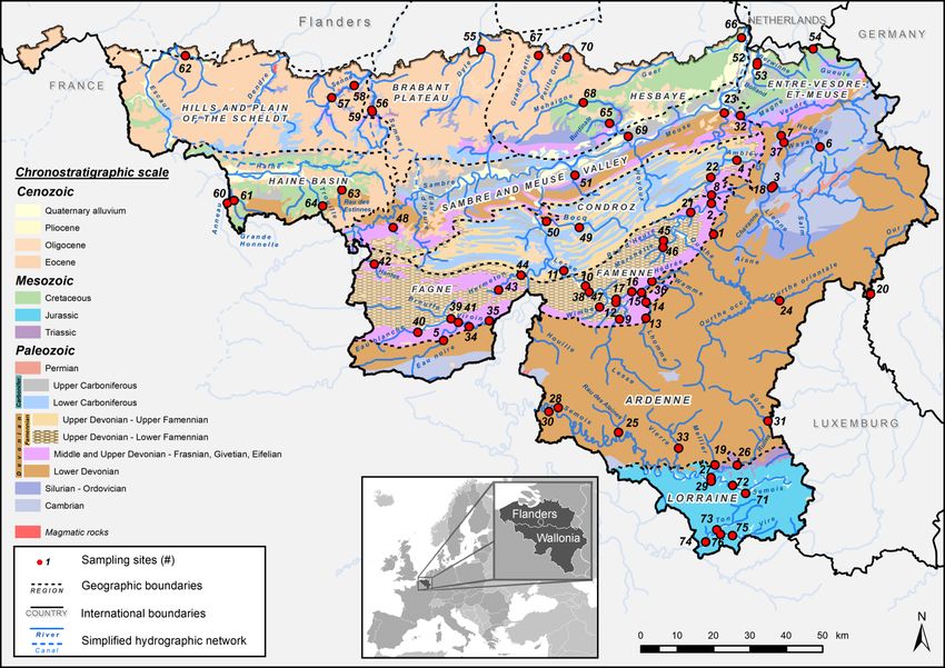
Water 2020, 12, 792 2 of 33

 In addition, depending on the threshold values used for the partial series method, there are
significant differences between the two procedures (Ta and Tp) for predicting a flood with low
recurrence [8]. To determine this threshold, a literature review was conducted in order to compare
the different threshold values and to confidently select a reliable method based on a series of
comparisons and tests.
 Most of the previous return period studies were based on daily discharge values because
hourly series were too short. Nowadays these records cover often longer than 30 years for some
hydrographic stations installed on upland rivers (Wallonia, Belgium). Given that on Ardennian
small catchments the most frequent floods are generally shorter than one day, it is preferable to work
with hourly discharge data. However, these records represent several hundred thousand unique
values, making peak flow identification difficult to calculate manually.
 Therefore, an automatic method of calculation in hourly discharge was developed. This method
makes it possible to identify hydrological independent events above the threshold and then
automatically calculate the characteristic flows.
 Most of the hydrology stations used in this paper have hydrologic series covering over more
than 30 years, which was essential to decrease the confidence interval of estimated return periods.
Indeed, the computation of return periods has to be based on a series of continuous hydrological
data over a sufficiently long period of daily flows or hourly flows. Woodyer [9] and Engeland et al.
[10] recommend 50‐year long series to reduce uncertainties in calculating the recurrence of
infrequent floods. The recommendations for the length of hydrological series are usually expressed
as daily data. However, unlike other meteorological data such as the amount of rainfall, the
autocorrelation of discharge data due to the high resolution [11] will not change the
recommendations because the watershed will always have a smoothing effect on the water level. It
should be noted that whilst hydrological series with duration between 30 to 50 years can be used,
caution should be exercised as the computed recurrences of extreme floods will be less reliable.
 As part of this study, the authors have compiled all observations of bankfull discharge of rivers
equipped with hydrographic stations. These field observations have supplemented or revised the
values presented in the literature [7,12–19]. In addition, these data sets enable prediction of rare
events. Given a sufficiently long duration of discharge series, we successfully estimated Q100‐flood
discharge. Moreover, extreme events have also been compiled, analyzed and compared to Q100
estimates. Maximum probable extreme floods were estimated from the catchment area by Guilcher
[20] and Réméniéras [21]. Recent data has been compiled using their methodology in order to
propose a robust value for the Myer–Coutagne equation [22] for the rivers of Wallonia.

2. Materials and Methods

2.1. Study Sites
 The study takes place in Wallonia, the southernmost region of Belgium. This mid‐latitude
region, with a Cfb climate, i.e., a warm‐temperate climate without dry season (oceanic type),
according to the updated Köppen–Geiger classification, experiences annual rainfall ranging from
725 mm in westermost Wallonia to 1400 mm in the Hautes Fagnes plateau [23]. In total, 76
hydrographic stations are considered in this study. On the non‐navigable rivers these stations are
managed by the Aqualim network and for those stations on the navigable waterways the SETHY
network is in charge. Both networks are entities of the Public Service of Wallonia (SPW). Since the
end of the 2000s, Aqualim stations record data in 10‐minute intervals which is then aggregated
hourly for their use and provision by the manager. The SETHY stations measure the water level
hourly. Undisclosed rating curves give hourly discharge data. The catchment area of these
limnigraphic stations ranges from 20 to 2,910 km². The oldest station recording hourly data was
installed in 1967; 37 stations offer data starting before 1990, 24 between 1990 and 2000, and 15 after
2000 (Table 1).
 The regional classification of stations depends on their location more specifically on their
sedimentary heritage, which is directly related to the local geology (Figure 1) of their catchment area

Water 2020, 12, 792 3 of 33

[7,24]. Of these stations, 37 have a regional affiliation to the Ardenne with impervious
schisto‐sandstone substratum of Cambrian‐Ordovician and lower Devonian (nos. 1 to 37). The
second group includes rivers located in the Fagne–Famenne region (nos. 38 to 47), a lithological
depression eroded into the lower Famennian and Frasnian soft shales. The third group comprises
rivers in the Condroz region (nos. 48 to 51) with Carboniferous limestone formations in depressions
and Upper Devonian sandstone formations on its ridges. The fourth group encompasses rivers in the
Entre‐Vesdre‐et‐Meuse region (nos. 52 to 54). Its geologic substratum is composed of Devonian
rocks, Cretaceous deposits and Meuse terraces area, with gravel‐bed rivers on moderately
permeable substrates.
 The fifth group incorporates the rivers located in the Brabant region (nos. 55 to 59), where
substratum is composed of Cambrian‐Ordovico‐Silurian formations under Eocene and Loessic
sandy cover. Hainaut rivers are the sixth group nos. 60 to 64); they are located in a silty area with
subsoil composed of Tertiary clay west of the Senne river and Cretaceous formations in the Haine
basin. Cretaceous chalk is also found in the Hesbaye region (nos. 65 to 70), covered by a thick layer of
loess.
 The eighth and last group encompasses Lorraine stations (nos. 71 to 76) with sandy‐loaded
rivers developed on Triassic and Lower Jurassic deposits of various kinds: conglomerates, marl and
sandstone, limestone, and sandy limestone.

 Figure 1. Location of the studied hydrological stations and simplified geological map of Wallonia
 (according to de Béthune [25] and Dejonghe [26], modified).

2.2. Bankfull Discharges of a Selection of Rivers in the Meuse and Scheldt Basins
 Among the characteristics discharges, the bankfull discharge is one of the most important for
geomorphological and hydrological reasons [7]; it is indeed an integrator of a large number of basin
characteristics [16]. Williams [27] compiled 16 methods for determining this flow while Navratil [28]
compared several methods of determination of bankfull discharge magnitude and frequency in
gravel‐bed rivers. The most common of them are: field observation at a hydrometric station
equipped with a stable rating curve, hydraulic geometry of the section [29,30], flood frequency

Water 2020, 12, 792 4 of 33

analysis, or a determination through Manning equation. Other authors analyze water level
time‐series in order to detect the overbank flow [31].
 The safest method is to observe the bankfull discharge in the field, preferably in a natural area
[27]. We used this way of determination Qb values for selected rivers.
 In most stable alluvial channels, it is generally accepted that the recurrence of Qb ranges
between 1 and 2 years, expressed in annual series [27,32–36]. Dury [37] considered that the return
period of Qb was equal to 1.58 years, the value corresponding to the most probable value of the
annual maximum in the Gumbel distribution. Tricart [38] assumed a recurrence of Qb equivalent to
1.5 years. However, Petit and Daxhelet [12] demonstrated that it increases with catchment size,
annual rainfall, contrast of the hydrologic regime, while it decreases with bed load sediment grain
size. Amoros and Petts [39] and Edwards et al. [40] estimate the recurrence of Qb at 1.5 years but
closer to one year for rivers with an impervious substrate and closer to 2 years in permeable terrain
area. Wilkerson [41] also postulates that the 2‐year recurrence flood (Q2) can be a good estimate of Qb
in absence of field observations.

 Table 1. Hydrological parameters of the studied stations

 Station
 Station Qb Specific Qb
ID River Location A (km²) start Ny Sources of Qb observation
 code (m3.s−1) (m3.s−1.km−2)
 date
 ARDENNE Region
 1 Aisne Erezée 67.4 L6690 1998–12 20 7.3 0.108 Houbrechts (2000) [14]
 2 Aisne Juzaine 183 L5491 1975–03 34 23.8 0.130 Houbrechts (2000) [14]
 3 Amblève Targnon 802.9 S6671 1968–06 20 87.3 0.109 New observation
 4 Amblève Martinrive 1062 S6621 1968–10 45 140 0.132 Houbrechts (2005) [42]
 5 Eau Noire Couvin 176 S9071 1968–03 33 36.9 0.210 New observation (2008)
 6 Hoëgne Belleheid 20 S6526 1993–06 25 10 0.500 New observation (2019)
 7 Hoëgne Theux 189 L5860 1979–02 36 36.8 0.195 Deroanne (1995) [43]
 8 Lembrée Vieuxville 51 L6300 1991–09 26 7.9 0.155 Houbrechts (2005) [42]
 9 Lesse Resteigne 345 L5021 1992–06 46 33 0.096 Franchimont (1993) [44]
 Bioengineering techniques report
10 Lesse Hérock 1156 L6610 1996–05 23 105 0.091
 (2016)
 Bioengineering techniques report
11 Lesse Gendron 1286 S8221 1968–01 51 131 0.102
 (2016)
12 Lesse Eprave 419 L5080 1969–01 41 37 0.088 Petit et al. (2015) [45]
13 Lhomme Grupont 179.9 L6360 1991–10 22 20 0.111 Franchimont (1993) [44]
14 Lhomme Forrières 247 L6310 1991–10 24 24.5 1 0.099 Computed Q0.625
15 Lhomme Jemelle 276 S8527 1969–01 50 29.71 0.108 Computed Q0.625
16 Lhomme Rochefort 424.9 L6650 1996–07 22 51.81 0.122 Computed Q0.625
17 Lhomme Eprave 478 L6360 1992–07 24 60 0.126 Petit et al. (2015) [45]
 Houbrechts (2005) [42] and new
18 Lienne Lorcé 147 L6240 1992–09 25 21.3 0.145
 authors observation (2008)
19 Mellier Marbehan 62 L5500 1974–06 39 8.8 0.142 New observation (2008)
20 Our Ouren 386 L6330 1991–09 26 29.2 0.076 New observation (2005)
21 Ourthe Durbuy 1285 S5953 1994–12 24 100 0.078 New observation
22 Ourthe Tabreux 1597 S5921 1970–12 48 160 0.100 Petit & Daxhelet (1989) [12]
23 Ourthe Sauheid 2910 S5826 1974–01 45 300 0.103 Pauquet & Petit (1993) [46]
 Ourthe
24 Houffalize 179 L5930 1979–02 37 21 0.117 Petit et al. (2015) [45]
 orientale
 Ruisseau Auby‐sur‐Semo
25 88.4 L6990 2003–09 15 13.3 0.150 New observation (2018)
 des Aleines is
 Habay‐la‐Vieill
26 Rulles 96 L5970 1981–11 33 11 0.115 Petit and Pauquet (1997) [7]
 e
27 Rulles Tintigny 219 L5220 1971–02 39 24.3 0.111 New observation (2008)

Water 2020, 12, 792 5 of 33

 Ry du Vresse‐sur‐Sem
28 61.8 L7000 2003–09 15 5.8 0.094 Jacquemin [47]
 Moulin ois
29 Semois Tintigny 380.9 S9561 1974–01 45 40 0.105 New observation (2008)
 Petit & Pauquet (1997) [7], Gob et al.
30 Semois Membre Pont 1235 S9434 1968–01 51 130 0.105
 (2005) [48]
31 Sûre Martelange 209 L5610 1975–03 40 32 0.153 Peeters et al. (2018) [19]
32 Vesdre Chaudfontaine 683 S6228 1975–06 43 120 0.176 Petit & Daxhelet (1989) [12]
33 Vierre Suxy 219.8 L7140 2003–12 15 19 0.086 New observation (2008)
 Olloy‐sur‐Viroi
34 Viroin 491 L6380 1992–01 26 55 0.112 New observation (2011)
 n
35 Viroin Treignes 548 S9021 1968–01 45 62 0.113 New observation (2009)
 L6370/
36 Wamme Hargimont 80 2011–06 13 12.1 0.151 New observation (2008)
 L7640
37 Wayai Spixhe 93.8 L6790 2002–03 17 25 0.267 New estimate
 FAGNE – FAMENNE Region
38 Biran Wanlin 51.9 L7190 2004–09 14 6.3 0.121 New observation (2008)
39 Brouffe Mariembourg 80 S9111 1981–01 38 20 0.250 New observation (2009)
 Eau
40 Aublain 106.2 L6530 1994–03 24 17 0.160 New observation (2011)
 Blanche
 Eau Vanderheyden [49] and new
41 Nismes 254 S9081 1968–01 50 29 0.114
 Blanche observation (2013)
42 Hantes Beaumont 92.4 L6880 2003–03 15 15 0.162 New observation
43 Hermeton Romedenne 115 L5060 1969–02 48 17.3 0.150 New observation (2008)
44 Hermeton Hastière 166 S8622 1967–09 50 20 0.120 New observation (2008)
 Marche‐en‐Fam
45 Marchette 48.9 L7120 2003–12 15 7.2 0.147 Petit & Daxhelet (1989) [12]
 enne
 Ruisseau
46 Baillonville 68 L6050 1984–06 29 14 0.206 Louette (1995) [13]
 dʹHeure
 Lavaux‐Sainte‐
47 Wimbe 93 L6270 1991–08 26 11.71 0.125 Computed Q0.625
 Anne
 CONDROZ Region
 Biesme Biesme‐sous‐Th
48 79.8 L7180 2004–09 14 6 0.075 New observation
 lʹEau uin
49 Bocq Spontin2 163.6 L7320 2006–04 40 18.3 0.112 Petit et al. (2015) [45]
50 Bocq Yvoir 230 L5800 1979–02 39 26.3 0.114 Peeters et al. (2013) [50]
51 Samson Mozet 108.2 L5980 1982–10 26 10.61 0.098 Computed Q0.625
 ENTRE–VESDRE–ET–MEUSE Region
52 Berwinne Dalhem 118 L6390 1991–12 24 17 0.144 Houbrechts et al. (2015) [51]
53 Bolland Dalhem 29.3 L6770 2001–12 17 3.4 0.116 New observation
54 Gueule Sippenaken 121 L6660 1996–06 22 16 0.132 Mols (2004) [52]
 BRABANT Region
55 Dyle Florival 430 L6160 1992–07 23 20.5 0.048 New observation (2011)
56 Samme Ronquières 135 S2371 1971–08 30 15 0.111 Denis et al. (2014) [53]
57 Senne Steenkerque 116 L5660 1996–06 40 14 0.121 SPW data
58 Senne Quenast 169 1977–03 40 19.5 0.115 New observation (2011)
59 Sennette Ronquières 70 L5670 1977–07 28 6 0.086 SPW data
 HAINAUT Region
60 Anneau Marchipont 78.2 L6870 2003–03 15 7.31 0.094 Computed Q0.625
 Grande
61 Baisieux 121 L5170 1971–01 40 12.41 0.103 Computed Q0.625
 Honnelle
62 Rhosnes Amougies 165 L5412 1972–02 38 19 0.115 SPW data
 Ruisseau
63 des Estinnes‐au‐Val 28.7 L7080 2003–11 15 3.01 0.105 Computed Q0.625
 Estinnes

Water 2020, 12, 792 6 of 33

64 Trouille Givry 55.7 L6710 2000–05 19 4.21 0.075 Computed Q0.625
 HESBAYE Region
65 Burdinale Marneffe 26.8 L6461 2008–09 10 2.21 0.082 Computed Q0.625
66 Geer Eben‐Emael 452.3 L6340 1991–08 23 11.9 0.026 Mabille & Petit (1987) [54]
 Grande Sainte‐Marie‐G
67 135 L5720 1978–01 41 10 0.074 New observation (2011)
 Gette eest
68 Mehaigne Ambresin 194.7 L6470 1991–12 25 12 0.062 Peeters et al. (2018) [19]
69 Mehaigne Wanze 352 L5820 1978–12 39 18.1 0.051 Perpinien (1998) [55] at Moha
70 Petite Gette Opheylissem 134 L6280 1991–08 25 4.81 0.081 Computed Q0.625
 LORRAINE Region
71 Semois Chantemelle 89 L5880 1979–01 40 11.1 0.125 New observation (2001)
72 Semois Etalle 123.9 L6180 1992–09 25 15.2 0.123 New observation (2008)
73 Ton Virton 89 L6440 1991–08 25 6.5 0.073 New observation (2007)
74 Ton Harnoncourt 293 L5520 1974–03 44 27.6 0.094 New observation (2008)
75 Vire Ruette 104 L5600 1975–07 39 21.3 0.205 SPW data and new estimate
76 Vire Latour 125 L6030 1983–10 34 12 0.096 New observation (2008)
 Columns legend: A (km²) is the catchment area at the station location; Qb max (m3.s−1) is field‐observed
 bankfull discharge expressed in hourly flow, 1except for values computed from partial series (Q0.625).
 2The Bocq station at Spontin presents incomplete hydrological data. A correlation with the SETHY

 station from Bocq at Yvoir was used to complete the data between 1978 and 2018.

 Petit and Pauquet [7] with further investigations by Petit et al. [16] proposed a relationship
between bankfull discharge and watershed area for pebble‐bedded rivers on impermeable
substrates (Ardenne’s rivers sensu stricto, Equation 1).
 .
 0.128 (R² = 0.961; n = 38) (1)
 As this equation is only available for Ardenne’s rivers, another type of estimation, based on
discharge series and recurrence intervals, will be presented below, applicable to all rivers. It should
be noted that this equation was computed from daily discharge series. With the refinement afforded
by bankfull discharge values expressed in hourly series resulting from field observations which have
been updated since Petit et al. [17] published their data (Table 1), the equation has been significantly
updated (Equation 2).
 .
 0.337 (R² = 0.908; n = 34) (2)

2.3. Methods for Flood Return Period Estimation

2.3.1. Graphical Method and Gumbel Distribution
 When dealing with flood frequency analysis and recurrence estimation, several methods exist.
The simplest method is graphical representation using a straight‐line fitting the flood discharge
value and the expression of the quantile. This graph linearizes the relation between the quantile x
and the cumulative frequency F on a probability scale [56]. Among many two‐parameter
distributions, the Gumbel law was selected for its ease of use. By inserting the reduced variable u in
the expression for the Gumbel distribution (u = ‐ln(‐ln(F))), it is possible to plot discharge values on
the axes x‐u and find the best fit straight line. Empirical frequency of a given discharge value can be
obtained thanks to the following equation (Equation 3)
 
 (3)
 1 2 
where n is the sample size, x[r] the value correspoding to the rank r and c a coefficient, usually fixed
to 0.5 after Hazen [57] and recommended by Brunet‐Moret [58].
 Fisher and Tippett [59] developed an analysis of extreme values frequency distribution. It was
applied by Gumbel [60,61] in the fields of hydrology and meteorology for discharge and rainfall

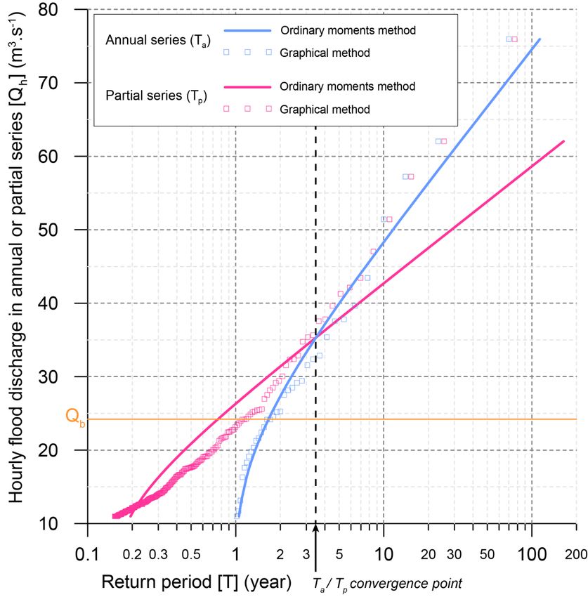
Water 2020, 12, 792 7 of 33

frequency analysis. The probability density of the Gumbel distribution is described by Equation 4,
considering Q as the flow variable.
 where (4)
 The variable 1/a corresponds to the scale parameter, characterizing the spreading of the values.
It is calculated from the standard deviation s of the sample (Equation 5). Parameter Q0 is a position
parameter which corresponds to the distribution mode and is calculated from the mean annual
discharge (Qm) of the series (Equation 6).
 1
 0.78 (5)
 
 1
 0,577 (6)
 
 The distribution function is represented by Equations 7 and 8.

 (7)

 (8)

 The implementation of the Gumbel distribution can be carried out according to different types
of adjustments to calculate the different parameters of the distribution. This results in the estimation
of the probability of occurrence of a given flood discharge [62]. Figure 2 presents an example
comparing the graphical method of analysing the annual and partial floods of the Aisne River at
Juzaine (ID no. 2) and the Gumbel ordinary moment method, which consists in equalizing the actual
moments of the flood samples and the theoretical moments predicted by Gumbelʹs law. This figure
shows that for partial series the best method is the graphical method as it gives correct return
periods for recurrence under 3.5 years. The graphical method is more appropriate for annual series
above this threshold. Tests were made using a large sample of rivers which led to the conclusion that
recurrence intervals have to be computed in partial series for a return period under 5 years and an
annual series above 5 years. This is because a comparison of the two methods reveals that, in a
partial series, the method of ordinary moments moves away from the points displayed when using
the graphical method. This 5‐year threshold found in this study is consistent with the data found in
the literature [63].

 Figure 2. Convergence of annual and partial series—comparison of the method of ordinary moments
 and the graphical method (example on the Aisne River at Juzaine—station no. 2).

Water 2020, 12, 792 8 of 33

 With data samples, the standard estimators of the mean and variance are given by Equation 9
and 10.

 1
 (9)
 
 1
 (10)
 1

 The theoretical expectation and variance of Gumbelʹs law are given by Equations 11 and 12
respectively. γ is the Euler constant (≅ 0.577) as reminded by Bernier [64].
 1
 γ Q (11)
 
 1
 (12)
 6 
 It is possible to calculate the asymmetric confidence interval of discharges with a given return
period by referring to Equation 13 and a chart giving the values T1 and T2, respectively the upper
and lower limits of the interval [65]

 ∈ (13)
with Qi, the theoretical discharge of a flood with a return period of i years and σ the standard
deviation of the floods sample used.
 Using the river stations samples, ensuring the observations are independent of each other, the
annual flood series (Ta), corresponding to the maximum annual flood, and the partial flood series
(Tp) whose flow is greater than a given threshold were analyzed.

2.3.2. Flood Return Period Calculation in Annual Series
 The Gumbel’s ordinary moment method was implemented on the series of 76 hydrological
stations (Figure 1) spread over the whole territory of Wallonia. For consistency with the work
already conducted in the study area, we have worked in calendar years. A small number of authors
undertake work in hydrological years, usually from July to June [66]. In the calculation of annual
flood series, the extreme variable used corresponds to the maximum observed annual flow. Because
this random variable is independent, it is extremely rare that the maximum flow in one year can
either influence the maximum flow in the following year or be influenced by the maximum flow in
the previous year. In case any problem is encountered whilst taking measurements at any of the
stations (due to technical failure, unstable rating curve, vandalism, ...), any hourly annual series with
missing data is only taken into account if: (1) at least 80% of the discharge data is available; and (2)
the maximum flood discharge measured during any incomplete year is not lower than the lowest
maximum annual flood discharge during the complete years.

2.3.3. Flood Return Period Calculation in Partial Series
 As annual series use only the maximum flood discharge per year, Langbein [67] when
calculating recurrences with a partial series developed the use of a more extensive flood sample,
selecting several flood peaks per year. All floods above a given threshold, independent of each other,
are selected as a variable. This leads to the difficulty, when making calculations using a partial series,
of determining a discharge threshold above which floods are used; and the time interval between
two flood events must be defined in order to consider them independently of each other [2,68].
Indeed, when several flood peaks occur in a short period of time, only the largest peak should be
retained [69].
 Table 2 presents the thresholds and intervals given by different authors in the literature. For
Dunne and Leopold [70], the threshold used for partial series may be the lowest maximum annual

Water 2020, 12, 792 9 of 33

flood in the data series. Ashkar and Rousselle [71] propose to use a threshold that is related to the
bankfull discharge, also recommended by Pauquet and Petit [46].
For Lang et al. [68], there is no unambiguous threshold value, but rather a range of threshold values
leading to similar recurrence calculations. This also applies to the subjectivity of the criterion of flood
independence. Physical parameters such as soil saturation in the catchment area modify the
responsiveness of rivers to rainfall [72] and therefore the duration of the time interval between two
successive peaks [73]. The flood selection methods for partial series recurrence computation are
quite variable as shown in Table 2 and depend on time intervals that are either related [66,74] or not
related [46,75,76] to the watershed physical parameters. Other authors use iterative statistical tests to
select n annual mean flood peaks [77,78]. These works have systematically been carried out on daily
flows, which greatly facilitates data analysis.

 Table 2. Flow thresholds and time intervals between floods considered as independent in partial
 series

 Threshold Time interval Author(s)
 Threshold corresponding to a flow Dalrymple, 1960
 ‐
 rate with a Tp of 1.15 years [80]
 Two successive peaks considered as
Threshold defining a number of 1.65
 independent if the flow drops to less than
N of floods where N represents the
 two‐thirds of the first peak. Interval greater Cunnane, 1973 [76]
 number of years recorded in the
 than three times the duration of the flood rise of
 discharge series
 the first five ‘clear’ hydrographs in the series
Lowest annual maximum flood of the Dunne and
 ‐
 series Leopold, 1978 [70]
 Two successive peaks considered as
independent if flow rate drops below Peaks separated by at least 5 days + the natural
 USWRC, 1976 [74]
 75% of the discharge of the lowest logarithm of the watershed surface (in miles²)
 peak
Threshold depending on the interval Selection by statistical self‐correlation test of
 Miquel, 1984 [73]
 optimized by autocorrelation test flood duration
 Threshold corresponding to a flow
 Irvine and Waylen
 rate with partial return period in the ‐
 [77]
 range 1.2‐2 years
 Time interval between two successive
 maximum flow rates equals to at least four Pauquet and Petit,
 0.6 Qb days, separated by a minimum whose value is 1993 [46]; Petit and
 less than or equal to 50% of the value of the Pauquet, 1997 [7]
 lower of these two maximums
 Several methods for estimating the
 Lang et al., 1999
threshold based on a stationarity test ‐
 [68]
 of the number of defined floods
 Adamowski, 2000
 Threshold and time interval defined to obtain between 2 to 5 floods peaks per year
 [78]
Threshold = μq + 3q where μq is the
mean daily flow rate of the series and
 Iterative high‐pass filtering of the daily flow Claps and Laio,
 q is the standard deviation of the
 rates in order to detect independent peaks 2003 [81]
daily flow rate according to Rosbjerg
 et al. [79]
 Brodie and Khan,
 Threshold = average daily flow rate 3 days
 2016 [75]
 Karim et al., 2017
 ‐ 10 to 15 days depending on watershed area
 [66]

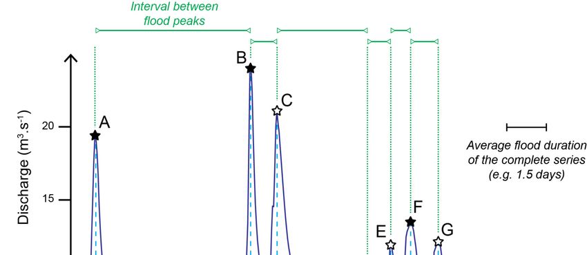
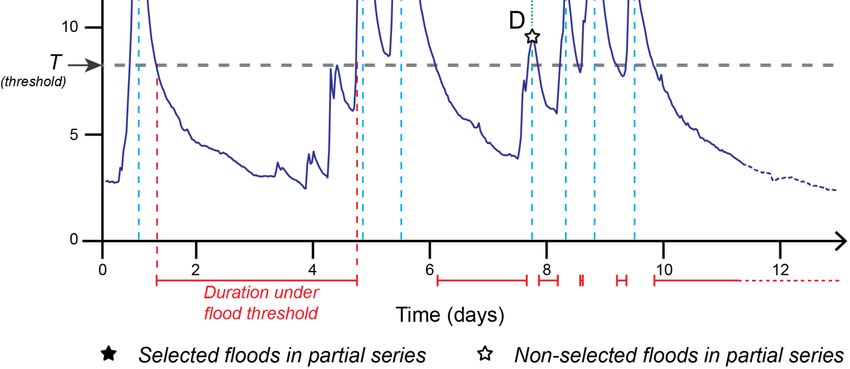
Water 2020, 12, 792 10 of 33

 Figure 3. Principle of selection of peaks over threshold (POT) in partial series.

 An automatic algorithm has been developed, based on hourly flood series, for extracting floods
above a given threshold and selecting independent floods. The VisualBasic script developed in
Microsoft Excel extracts temporal flood data (start and end date of the flood, duration, date of the
observed maximum flow, time interval from the previous peak and time interval below the
threshold between two successive floods). The code of this algorithm is available as Supplementary
Material and on the website of the Hydrography and Fluvial Geomorphology Research Centre of the
University of Liège (http://www.lhgf.uliege.be/). The maximum flow rate of each flood at the
hydrograph station above the tested threshold is extracted and some statistical variables, such as the
average duration of floods are calculated. Figure 3 shows in graphical form the different time
parameters between the successive floods, named A to G in this example.
 If several peaks are observed successively during the above‐threshold period (Figure 3: B and
C), only the maximum peak will be used (B). A flood peak that is separated from the previous one by
a time interval less than the average duration of all the peak discharges above threshold will not be
used in the calculation of the partial series (E and G not retained). In addition, to ensure flood
independence in the calculation of partial series, a moving window operating on three successive
above‐threshold areas (D‐E‐F or E‐F‐G for example) will only retain the largest flood (F).
 According to the literature, several tests were performed in peaks over threshold (POT)
calculation and in the threshold selection: (1) the lowest annual maximum flood of the series [70]; (2)
a fraction of the bankfull discharge (from 0.4 to 0.8 Qb, encompassing the 0.6 Qb value proposed by
Petit and Pauquet [7]); (3) a wide range of specific discharges (from 0.025 to 0.2 m3.s−1.km−2); (4)
several characteristic discharges estimated from hydrologic series; and (5) a discharge threshold
defined to obtain around 5 independent flood peaks per year [78].
 These methods each have methodological issues [40]. (1) The lowest annual maximum flood is
dependent on the length of the hydrological series. A historical severe drought (1976, 2003, or 2018

Water 2020, 12, 792 11 of 33

depending on the location in Belgium [82]) will usually be the lowest annual maximum flood in our
data. The designated threshold will be a little too high for stations with hydrologic series that do not
go back to this year of severe drought, making recurrences calculated using this incomplete data,
when compared with stations with hydrological data including those years of severe drought not
comparable with each other. (2) A threshold which is defined from a percentage of the bankfull
discharge value (e.g., 0.6 Qb) is not suitable in the absence of field observations, as the data
sometimes do not exist. (3) Specific discharges as threshold for POT calculations are not suitable
because permeable and impervious watersheds will show major differences in their specific
discharges [83]. (4) A characteristic discharge value such as Q2.33 could be set as threshold but it is
also dependent on the length of the hydrologic series and the type of fluvial regime and substratum.
(5) The best series‐length independent estimator we have used is the number of average flood peaks.
Adamowski [78] suggests using 2–5 peaks while Cunnane [76] opts for a threshold a number of 1.65
N of flood peaks where N represents the number of years recorded in the discharge series while
Lang et al. [68] utilize an equation which will test both the dispersion and the stationarity of the
number of floods. We have chosen to set a threshold that gives a value of around 5 independent
peak floods after POT selection. As the selection algorithm computer software takes time to run,
another type of algorithm has been conceived in order to count all peak floods (dependent and
independent) in real time. The threshold that gives 5.5 dependent and independent peak floods per
year for each station has been sought; it corresponds to about 5 independent flood peaks per year
and does not require the complete operational run of the algorithm (Table 3). The scripts are
available in the Supplementary Materials.

3. Results

3.1. Bankfull Discharge Return Period Analysis
 While the computation of the flood frequency in annual series is only dependent upon the
lowest annual flood, the newly developed algorithm for extracting peaks over threshold in partial
series gave us the possibility to test a greater number of threshold parameters across a wide range of
stations. It gives a precise idea of the behaviour of any return period of a given flood discharge value
in relationship with the number of flood events per year. This method showed that an average
number of 5 independent events per year (corresponding roughly to 5.5 dependent and independent
events per year) will give a return period value that is not only consistent with field observation but
also less sensitive to a threshold value change.
 Tests were performed to assess the statistical utility of working with hourly discharges instead
of daily discharges in relation to the area of the catchment. A seasonal difference is noticeable, winter
floods require hourly discharge series for watersheds with an area lower than 250 km² in Wallonia
while summer floods require hourly discharge values for a catchment area of less than 100 to 250
km², depending on the area and the fluvial regime.
 The analysis of the return period of Qb by region needs at first an overview of the regional
specific bankfull discharge. The lowest values are observed in rivers from Hesbaye with an average
specific Qb of 0.063 m3.s−1.km−2. Rivers from Brabant, Hainaut, and Condroz regions show average
values of 0.096, 0.098, and 0.100 m3.s−1.km−2 respectively. The rivers from Lorraine exhibit average
specific Qb discharge value of 0.119 m3.s−1.km−2 while Entre‐Vesdre‐et‐Meuse and Ardenne regions
are showing values of 0.131 and 0.132 m3.s−1.km−2 respectively. Larger values are observed in the
region of Fagne and Famenne with 0.156 m3.s−1.km−2. Two groups are clearly distinctive: the
Fagne–Famenne with systematically higher Qb values, the Hesbaye with systematically lower Qb. At
river scale, some of them clearly stand out. We can cite the ones with a specific bankfull discharge
value above 0.2 m3.s−1.km−2; in Ardenne region: the Eau Noire (no. 5), Hoëgne river (no. 6) and Wayai
river (no. 37); in Fagne–Famenne region: Brouffe river (no. 39) and the Ruisseau d’Heure (no. 46).
The Hoëgne River at Belleheid (no. 6) appears clearly as an outlier. It is located in a cascade‐system
reach with a steep profile slope (average: 3.7%) [84]. Its observed Qb value (~10 m3.s−1) is equal to the
Q0.625 computed value (9.9 m3.s−1). However this value is very different from the 2.4 m3.s−1 given by

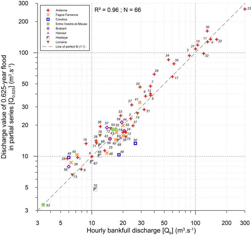
Water 2020, 12, 792 12 of 33

the Equation 1 for pebble‐bedded rivers on impervious substratum [16]. The Brouffe River located in
the Fagne region with a specific Qb value of 0.250 m3.s−1.km−2 correspond to an anthropized reach in
the vicinity of the gauging station. The other rivers from Fagne–Famenne region show specific Qb
values in the range 0.1–0.2 m3.s−1.km−2.
 Based on the return period computation with an average number of 5 events per year, we used
the least square method to find which flood frequency could represent the field‐observed bankfull
discharge. Tests performed with 65 Qb values led the authors to consider that the Q0.625‐flood is the
most suitable value, ie. flood events happening 1.6 times a year. Figure 4 shows that the fit between
Q0.625 and Qb does not exhibit the normal regional pattern because the computation is taking into
account both the physical features as well as the hydrological parameters. In addition, with their
more extensive watershed catchment areas, Ardenne’s rivers are those with the largest Qb in this
dataset. A few outliers are detected: no. 49 and no. 50, the Bocq River whose stations suffer from
rating curve instability, lack of data and concrete‐channelized reaches near hydrographic stations.

 Figure 4. Fit between the discharge value of Q0.625 in partial series and the field‐observed Qb.

 Tests carried out on the database of selected Walloon rivers have shown a convergence
occurring for a return period of 5 years on average (Table 3), as shown by the example of the Aisne at
Juzaine (station no. 2 ‐ Figure 2). Whilst Ardenne, Condroz, and Fagne–Famenne rivers show a
converging value around 4.6 years; in contrast to sand‐ and silt‐bedded rivers of the regions Lorraine
and Brabant which present average values of 11.8 and 10.5 respectively. Taking into account these
observations, return periods of bankfull discharges will correspond to the value deducted from the
partial series if it is less than 5 years, and will be expressed by the value deducted from the annual
series above this threshold (see Table 3).
 Ardenne rivers present an average bankfull discharge recurrence interval of 0.6 years without
clear link to their watershed area. The rivers from Entre‐Vesdre‐et‐Meuse show a value around 0.5
years. Whilst Brabant, Fagne–Famenne and Lorraine rivers have average values of 0.7 years. In
contrast, the rivers from Condroz and Hesbaye reach an average bankfull discharge return period of
2.6 and 2.7 years respectively.

Water 2020, 12, 792 13 of 33

 Table 3. Return period of characteristic discharges computed for the selection of hydrologic stations

 Annual series Partial series Ta/Tp
 Annual Threshold conver‐
 Ta Ta Tp
 lowest Q100 for 5.5 Q0.625 gence
ID River Location Qb (m3.s−1) Qb 3 ‐1 Qhmax Qb
 flood (m .s ) events/yr (m3.s−1) point
 (yr) (yr) (y)
 3 −
 (m .s )1 −
 (m .s )
 3 1 (yr)
 ARDENNE Region
 1 Aisne Erezée 7.3 7.1 1.1 25.8 32 6.30 0.30 9.7 4.0
 2 Aisne Juzaine 23.8 11.0 1.6 74.6 >100 13.15 0.68 23.0 4.0
 3 Amblève Targnon 87.3 78.1 1.4 250.7 75 60.00 0.51 93.6 5.0
 4 Amblève Martinrive 140 74.4 1.6 411.9 54 84.15 0.70 134.9 4.5
 5 Eau Noire Couvin 36.9 26.9 1.4 129.1 37 20.68 0.52 40.1 5.3
 6 Hoëgne Belleheid 10 6.1 1.5 27.6 44 6.05 0.62 9.9 3.5
 7 Hoëgne Theux 36.8 24.2 1.3 132.2 45 25.80 0.33 47.5 7.0
 8 Lembrée Vieuxville 7.9 3.8 1.6 25.7 70 3.62 0.71 7.5 4.0
 9 Lesse Resteigne 33 13.4 1.2 135.2 68 20.39 0.47 38.1 3.4
10 Lesse Hérock 105 80.5 1.3 397.2 52 69.39 0.46 118.6 3.4
11 Lesse Gendron 131 58.1 1.6 418.1 65 70.00 0.67 127.3 3.8
12 Lesse Eprave 37 14.0 1.5 120.1 >300 22.70 0.55 38.6 3.8
13 Lhomme Grupont 20 7.9 2.0 51.8 29 10.59 1.12 17.0 3.2
14 Lhomme Forrières 24.51 15.7 1.5 81.6 35 15.90 0.62 24.5 3.0
15 Lhomme Jemelle 29.71 12.4 1.4 87.9 30 17.77 0.62 29.7 3.9
16 Lhomme Rochefort 51.81 34.2 1.5 187.5 32 28.11 0.62 51.7 3.0
17 Lhomme Eprave 60 45.7 1.4 150.7 28 35.70 0.68 58.7 3.4
18 Lienne Lorcé 21.3 10.5 2.4 52.1 47 10.49 1.28 17.0 6.0
19 Mellier Marbehan 8.8 6.8 1.1 47.8 64 6.96 0.32 13.3 3.7
20 Our Ouren 29.2 31.4 1.0 138.4 37 22.10 0.28 46.6 5.5
21 Ourthe Durbuy 100 61.9 1.4 329.9 74 64.96 0.50 108.8 3.8
22 Ourthe Tabreux 160 68.1 1.9 450.2 77 73.80 1.03 134.5 3.7
23 Ourthe Sauheid 300 148.9 1.8 827.3 49 159.92 0.92 263.9 3.7
24 Ourthe orientale Houffalize 21 9.9 1.9 63.3 ~100 9.61 1.01 17.5 3.8
25 Ruisseau des Aleines Auby‐sur‐Semois 13.3 7.6 1.0 26.5 23 7.82 1.30 11.3 4.0
26 Rulles Habay‐la‐Vieille 11 6.9 1.1 43.5 32 7.80 0.38 14.1 3.7
27 Rulles Tintigny 24.3 20.3 1.0 74.5 30 17.40 0.33 31.3 20.0
28 Ry du Moulin Vresse‐sur‐Semois 5.8 7.3 1.0 31.4 55 6.02 0.31 9.5 2.7
29 Semois Tintigny 40 34.6 1.1 203.1 >100 34.80 0.29 62.0 4.0
30 Semois Membre Pont 130 89.0 1.2 555.3 ~100 80.90 0.41 162.3 3.5
31 Sûre Martelange 32 13.9 1.5 107.6 73 11.27 0.81 28.3 3.6
32 Vesdre Chaudfontaine 120 35.4 2.0 288.1 71 53.14 1.20 98.1 5.0
33 Vierre Suxy 19 15.3 1.1 92.3 33 11.52 0.41 24.7 3.3
34 Viroin Olloy‐sur‐Viroin 55 41.3 1.2 281.5 26 42.38 0.29 85.6 5.8
35 Viroin Treignes 62 47.4 1.3 259.8 141 43.79 0.37 78.1 3.7
36 Wamme Hargimont 12.1 9.8 1.3 63.3 89 11.76 0.26 19.4 6.0
37 Wayai Spixhe 25 14.4 2.0 63.1 >100 11.22 1.41 19.7 3.0
 FAGNE–FAMENNE Region
38 Biran Wanlin 6.3 4.2 1.1 30.6 14 3.96 0.35 8.7 3.0
39 Brouffe Mariembourg 20 7.3 1.9 50.6 75 7.47 1.30 15.7 3.5
40 Eau Blanche Aublain 17 9.3 1.7 48.4 37 8.03 1.00 14.5 3.2
41 Eau Blanche Nismes 29 20.1 1.4 96.6 >300 19.70 0.43 33.1 4.3
42 Hantes Beaumont 15 10.9 1.5 60.2 30 6.42 0.63 14.9 3.5
43 Hermeton Romedenne 17.3 9.0 1.7 50.5 75 8.61 0.66 17.0 7.5
44 Hermeton Hastière 20 11.3 1.4 65.2 87 9.53 0.64 19.9 4.0
45 Marchette Marche‐en‐Famenne 7.2 6.3 1.0 26.8 34 5.63 0.27 10.3 6.0
46 Ruisseau dʹHeure Baillonville 14 6.9 1.9 32.7 23 4.45 1.28 10.7 8.0

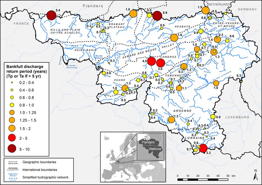
Water 2020, 12, 792 14 of 33

47 Wimbe Lavaux‐Sainte‐Anne 11.71 7.8 1.3 31.7 40 6.68 0.62 11.7 4.0
 CONDROZ Region
48 Biesme lʹEau Biesme‐sous‐Thuin 6 4.1 1.2 39.5 20 4.24 0.32 9.8 4.0
49 Bocq Spontin 18.3 4.3 3.3 47.3 >150 5.09 2.99 10.3 4.0
50 Bocq Yvoir 26.3 5.7 4.3 61.3 >150 6.81 4.53 13.3 4.0
51 Samson Mozet 10.61 6.3 1.5 30.3 21 6.00 0.62 10.6 6.5
 ENTRE‐VESDRE‐ET‐MEUSE Region
52 Berwinne Dalhem 17 13.3 1.5 60.1 >100 8.72 0.53 18.3 5.5
53 Bolland Dalhem 3.4 1.7 1.7 11.4 >150 2.07 0.62 3.4 3.7
54 Gueule Sippenaken 16 14.6 1.1 46.8 39 9.30 0.44 18.1 5.7
 BRABANT Region
55 Dyle Florival 20.5 13.5 2.6 31.2 16 12.70 1.77 17.6 20.0
56 Samme Ronquières 15 9.5 1.5 46.0 >100 8.28 0.66 14.7 4.0
57 Senne Steenkerque 14 8.8 1.1 51.0 ~100 9.18 0.32 18.9 9.0
58 Senne Quenast 19.5 9.9 1.3 57.4 ~100 10.39 0.49 21.3 9.0
59 Sennette Ronquières 6 4.2 1.2 19.4 68 3.94 0.34 7.9 >50.0
 HAINAUT Region
60 Anneau Marchipont 7.31 2.6 1.8 33.9 79 2.96 0.62 7.3 5.0
61 Grande Honnelle Baisieux 12.41 3.3 1.6 46.1 44 5.46 0.62 12.4 4.8
62 Rhosnes Amougies 19 7.3 5.42 28.2 50 10.90 3.98 15.0 9.0
63 Ruisseau des Estinnes Estinnes‐au‐Val 3.01 0.6 1.9 15.2 >100 1.26 0.62 3.0 3.6
64 Trouille Givry 4.21 1.1 1.8 17.6 51 1.69 0.62 4.2 6.2
 HESBAYE Region
65 Burdinale Marneffe 2.21 0.9 1.8 7.6 30 0.92 0.62 2.2 5.5
66 Geer Eben‐Emael 11.9 6.4 2.5 19.6 67 7.59 1.90 10.1 3.8
67 Grande Gette Sainte‐Marie‐Geest 10 3.1 1.7 36.3 50 4.68 0.81 8.8 4.0
68 Mehaigne Ambresin 12 5.8 1.5 29.4 22 7.43 0.49 12.8 10.4
69 Mehaigne Wanze 18.1 7.2 2.5 39.4 >100 9.10 1.63 14.2 4.5
70 Petite Gette Opheylissem 4.81 2.2 8.93 18.5 >300 2.64 18.46 4.8 4.0
 LORRAINE Region
71 Semois Chantemelle 11.1 6.7 1.3 32.9 44 8.05 0.35 13.3 6.4
72 Semois Etalle 15.2 12.8 1.2 40.2 38 12.48 0.31 18.4 6.5
73 Ton Virton 6.5 4.7 1.6 12.5 26 4.64 0.59 6.6 ~30.0
74 Ton Harnoncourt 27.6 11.4 2.0 84.4 376 15.31 0.75 25.8 7.0
75 Vire Ruette 21.3 6.7 3.2 40.4 41 8.01 2.16 15.3 15.0
76 Vire Latour 12 10.0 1.1 40.4 56 9.69 0.30 15.8 5.8
 Column legend: Qb is the bankfull discharge expressed in hourly flow,1except for values computed
 from partial series (Q0.625). 2The Rhosnes River at Amougies and the 3Petite Gette River at
 Opheylissem are located in anthropized reaches. 4The Vesdre River at Chaudfontaine (no. 32) is
 disturbed by human dams upstream so return periods are not consistent with surrounding stations’
 values.

 Figure 5 maps the return period of field‐observed bankfull discharges for all stations where it
was evaluated. The most station‐populated rivers from our database comprise the Ourthe and the
Lesse watershed. Ourthe River and its tributaries present Qb return period from 0.3 to 1.3 years.
Stations located on the main watercourse of the Ourthe have an average value of 0.8 years while
Aisne tributary (stations no. 1 and no. 2) and Lienne tributary (station no. 18) show values of 0.30,
0.68 and 1.28 years respectively.
 In the case of the Lesse River and tributaries, most of the stations are located in the Famenne
region but they have a substratum heritage from the Ardenne region. Except for one station (no. 13,
Lhomme at Grupont with 1.13 years), the Lesse River and its tributaries show Qb return period from
0.3 to 0.7 years.
 Viroin River and its tributary the Eau Noire River have Qb discharge return period between 0.3
and 0.5 years (with Ardenne characteristics) while the Eau Blanche River and Brouffe River,

Water 2020, 12, 792 15 of 33

tributary of the Viroin and located in the Fagne region, show return period of 1.0 and 1.3 years
respectively.
 The Semois catchment and all its studied tributaries present Qb recurrence interval ranges
between 0.2 and 0.4 years, which is consistent with observations and flood alerts from the regional
river network manager. The Vire and Ton catchments show bankfull discharge return period from
0.3 to 0.7 years except for the Vire at Ruette (station no. 75) where natural levees increase the value to
2.2 years.
 Rivers from Entre‐Vesdre‐et‐Meuse have values between 0.4 and 0.6 years while the Mehaigne
catchment presents values from 0.5 years upstream (in the Hesbaye region sensu stricto) and 1.6 years
downstream in a reach where the watercourse is recharged with pebble bedload due to the local
Paleozoic substratum.
 In Brabant region, the Senne catchment including the Samme River presents values ranging
from 0.3 to 0.7 years. The Geer River and the Dyle River at locations under study present a value of
Qb return period of 1.9 and 1.8 years respectively. The other rivers have not‐often experienced
bankfull discharge events: the Petite Gette River with a Qb return period of 8.9 years, the Rhosnes at
Amougies with 5.4 years and the Bocq River at two locations (4.5 and 3.0 years). These discharge
patterns are directly linked to the high values of the specific discharges values described earlier. The
station corresponding to the Vesdre River at Chaudfontaine (no. 32) is not represented in graphs and
tables. The calculated return period of its discharges is disturbed by hydroelectric and drinking
water dams (Eupen and Gileppe dams).

 Figure 5. Return period of the observed bankfull discharge (expressed in partial series for values
 below 5 years and in annual series beyond).

3.2. Discharge and Return Period of Extreme Floods
 Extreme floods were defined on the basis of the maximum hourly discharges recorded during
the hydrological data series (see Table 3). The time frame for this recorded data is obviously
dependent on the date on which the station was installed and, to a lesser extent, it is sensitive to the
stability of the calibration curve [85].
 Many authors have compiled databases of extreme floods around the world [86] or for a
selection of countries such as the United Kingdom [8] and the United States [87] and relate these

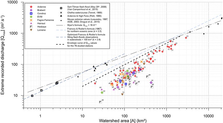
Water 2020, 12, 792 16 of 33

extreme discharges with watershed area. Figure 6 shows scatter points from hourly maximum
discharges observed in rivers from Wallonia in the recording period, ranging from the longest
timeframe of 1968 to 2018, to various other timelines, depending on station installation dates. On the
basis of the calculation of the 100‐year recurrence interval flood with the annual series (and therefore
independently of the previous methodological results), this figure also presents the relationship
between the centennial flood (Qa100, computed with Gumbel method’s of moments) and watershed
area (see Equation 14).
 .
 3 (14)
 Figure 6 also shows the extreme discharges estimated during catastrophic flash‐flood events in
ungauged catchments [88] utilizing a range of methods (specific stream power deducted from
mobilized bed load, maximum water level in channel, …) and the large centennial flood of the
Meuse River in 1925–26 in the valley of Liege [89] and a few observations of the well over 50‐year
return period of the Meuse River flood in Dec. 1993 in the French departments of Ardennes and
Meuse [90].
 The Myer’s formula is an equation (Equation 15) used in the computation of extreme floods
[2,20–22,91].

 C (15)
where Qmax is the maximum discharge (in m3.s‐1), A the watershed area, C the Myer’s rating which
relates to the physical parameters of the watershed and to the morphoclimatic system and the
exponent a = 0.5; the value of this exponent is justified by the fact that, in the presence of a uniform
downpour, the total volume flow is proportional to the area of the basin and the concentration time
is schematically equivalent to the length of the watercourse [2,92,93]. Myer’s ratings, which were
recorded following extreme floods in the High Fens range from 16 to 18 [94,95], with
pluri‐centennial return periods. In Corsica, Gob et al. [96] computed a Coutagne–Myer coefficient
close to 30 for the extreme flooding in 1973 in these Mediterranean mountains with their steep
slopes. This coefficient exceeds 100 in the Ardèche River and its tributaries during ‘Cévenoles’
episodes, because it is related both to meteorological and topoclimatological parameters, with the
energy of the topographic relief inducing a particular fluvial regime. Differences are partly
explained by the more important role attributed to the surface of the basin in Myerʹs formula, thus
accentuating the size differences between watersheds [93].
 Sart‐Tilman flash‐floods, Chefna watercourse and the largest contemporary floods of the Meuse
River confirm the Myer’s rating of 18 previously proposed on the basis of a more limited number of
observations (Figure 6).
 From a dataset of peak discharge of extreme floods observed in the last two centuries in 1,400
watersheds in the entire world, Francou and Rodier [97] presented an envelope curve based on the
given catchment area [88]. Their formula (Equation 16) gives the expected peak flow rate Q (in
m3.s−1) with A, the area of the watershed (in km²), Q0 = 106 and A0 = 108. The parameter k is a
regionalized parameter and it is equal to 3.5 in the northern oceanic zone.
 ‐
 Q A (16)
 Q A
 However, their dataset is mainly composed of large watersheds (from ~10 to 5,500,000 km²) and
a huge variability appears in their resulting plot points. They have identified, for any catchment with
less than 10, 20‐square‐kilometre areas, a limit named the “downpour phenomenon” where heavy
rainfall associated with runoff can lead to a specific discharge of 10 m3.s−1.km−2 [97]. Indeed, Francou
& Rodier’s equation seems most unsuitable for modelling extreme floods for any catchment area
below ~100 km² with k = 3.5 (Figure 6). A value of 3.9 is needed in order to fit with the extreme
discharge values that were observed in watercourses of Wallonia.

Water 2020, 12, 792 17 of 33

 Figure 6. Extreme recorded discharge between 1968 and 2018 in gauged Walloon rivers and the
 comparison between Myer’s formula (with C = 18) and different flash flood in ungauged watershed
 (Sart‐Tilman flash flood, Chefna watercourse and High Fens watercourses) as well as Meuse 1925‐26
 large inundation; envelope curve of Q100 values computed for the 76 studied stations. Francou &
 Rodier’s formula for northern oceanic zone maximum discharge is also shown as well as the
 optimized k parameter fitting with extreme floods of Walloon rivers.

 The Francou and Rodier’s equation, taking into account extreme floods for two centuries, is
significantly higher than, but parallel, to the Q100 envelope curve from our selection of 76 stations.
Their estimate of Q100 discharge is obviously related to the length of the series of observations and to
the extreme events that occurred in the watersheds in this study, given the large spatial disparity in
storm precipitation or snowmelt associated with the highest floods. With an average of 31 years of
data gathered by the 76 stations studied, the highest floods have an average recurrence of 80 years.
Several maximum flow rates are considered as a pluri‐centennial flood. The limited length of the
hydrologic series does not allow a more robust recurrence interval estimate. As mentioned earlier,
Francou and Rodier’s envelope curve significantly underestimates the discharge of the flash‐floods
which occurred in Belgium in both small and large watersheds. These events are markedly better
modeled by the Myer’s formula.

4. Discussion
 With daily series computation of both annual and partial series as datasets, Richards [8]
proposed the equation Ta = Tp + 0.5. In the analysis of a selection of rivers in different geographical
regions in Wallonia (Belgium), this equation turns into Ta = Tp + 0.83 (± 0.10 as standard deviation)
for bankfull discharge. The flood threshold in partial series has been defined—thanks to a complete
analysis of the evolution of the return period value—depending on the average number of flood
events per year. Each station has a graphic representation of the area where the calculated return
period is stable and corresponds, in our subset, to around five events per year. Comparing this to
other studies (see Table 2) which mention a threshold corresponding to a flow rate of either a
defined partial return period [77,80] or linked to a number of flood events per year [76,78], we use a
threshold (Tp ~ 0.2 years) lower than daily series studies (Tp from 1.15 to 2 years).
 As a result of Qb determination in hourly series and a threshold of Tp ~0.2 years, we have
observed that Qb value could be accurately estimated in absence of field data as the Q0.625 discharge
in partial series. Wilkerson [41] listed the published Qb return period of a variety of authors from
Europe, USA and Australia. They range from 0.46 to 10 years depending on localization, with

Water 2020, 12, 792 18 of 33

average or mode values often reported as being between 1.0 and 2.0 years because annual series are
mainly used. Petit [95] mentions that the use of partial series give a better estimation of the
reccurence interval of Qb and this is in the range from 0.4 to 0.7 years in Ardenne rivers with any
watershed area of less than 500 km². With the same hydrologic series, annual series give for our
subset (field‐observed data excluding anthropized stations) an average Qb return period value of 1.5
years (range: 1–2.6 yr) for 59 stations. Later studies have confirmed this value in Southern Italy [98]
in annual series. However recent literature lacks values in partial series over a wide selection of
stations [7,99,100].
 This study takes place more than 20 years after the reference study of Petit and Pauquet [7] for
the bankfull discharge recurrence interval in pebble‐bedded rivers on impermeable substratum.
They found that bankfull discharge recurrence interval for rivers with a hydrographic basin area of
less than 250 km² in annual series was of the order of 1 year, very close to the value limit which one
can obtain by using annual series and values around 1.5 to 2 years in the case of larger Ardenne type
rivers [7]. Fagne and Famenne rivers, often characterized by small catchment area due to the
morphology of the lithologic depression, show a large specific Qb. This is a consequence of the fact
that they flow over soft shales which are not very resistant to erosion [17,101], and this tends to
incise the river more deeply into its bed. However, these rivers exhibit Tp values of around 0.7 years.
Bankfull discharge frequency is just a bit more important than that of either the Ardenne rivers (0.6
years) or the Entre‐Vesdre‐et‐Meuse rivers (0.5 years). In the rivers of Hesbaye, a generalized
weakness of the flows (e.g., Gette and Geer Rivers) is observed, because precipitation is much lower
and anthropogenic withdrawals are far from negligible. Average bankfull discharge return period
reaches 2.7 years despite low specific Qb.
 Lorraine rivers have two different lithological contexts: the Ton River and the upstream part of
the Semois River flow on Sinemurian sandstone with a stabilized fluvial regime; the downstream
part of the Semois River which flows in a depression excavated in the marls, resulting in a highly
contrasted regime. The Vire River at the station of Ruette has natural levees inducing a high Qb
return period (2.16 years). Due to their similar substrate to Ardenne watercourses, the rivers of
Brabant— which is incised in Cambro‐Ordovico‐Silurian formations—do not deviate from the
relationship defined for the Ardenne. However, rivers such as the Senne, the Dyle are nevertheless
very different from the Ardenne rivers, even if they incise the substratum very locally. Very different
land use in their catchment can modify the hydrological response to precipitation [102].
 The Q100‐flood discharge and the return period of extreme floods were analyzed through
envelope‐curve based on maximum hourly discharges recorded during the hydrological data series
in the one hand, as well as literature detailing the available data for flash‐floods and extreme floods
in Wallonia and surrounding areas. A majority of flood time series are shorter than 50 years. This
leads to a mismatch between the length of the flood records and the need for an adequate estimate of
the return period, in order to achieve effective and efficient infrastructure design [10]. Increased
imperviousness of the landscape tends to increase watershed response to rainfall [102] and
heightens the risk of extreme flash‐floods [88].
 The Myer–Coutagne equation was used with updated data sets on extreme flood discharges in
Wallonia. Myer’s rating has been confirmed at 18 for extreme (flash‐)floods in catchments with an
area from 0.6 to 20,000 km². The difference between the Q100 floods observed in gauged stations and
the maximum discharge (Qmax) estimated with the Myer’s rating varies with the size of the
catchments and the length of the hydrographic series.
 Climate projections indicate that in many regions of the world the risk of increased flooding or
more severe droughts will be higher in the future [103]. While no significant changes were detected
in annual rainfall series since an abrupt break in 1909 in Uccle (centre of Belgium) [104], winter
precipitations show several increases from 1833–1909, 1910–1987, and 1988–2007. In this changing
environment, there is a mismatch between the desire to have long series of data to obtain better
estimates of characteristic discharge (minimum annual flood, Q100, ...) and the problem linked to
changes in climatological normal—that have to be reassessed over the last 30 years [105]—as
prescribed by the World Meteorological Organization.