BVOC-aerosol-climate feedbacks investigated using NorESM - Atmos. Chem. Phys
←
→
Page content transcription
If your browser does not render page correctly, please read the page content below
Atmos. Chem. Phys., 19, 4763–4782, 2019
https://doi.org/10.5194/acp-19-4763-2019
© Author(s) 2019. This work is distributed under
the Creative Commons Attribution 4.0 License.

BVOC–aerosol–climate feedbacks investigated using NorESM
Moa K. Sporre1 , Sara M. Blichner1 , Inger H. H. Karset1 , Risto Makkonen2,3 , and Terje K. Berntsen1,4
1 Department    of Geosciences, University of Oslo, Oslo, Norway
2 Climate   System Research, Finnish Meteorological Institute, P.O. Box 503, Helsinki, Finland
3 Institute for Atmospheric and Earth System Research/Physics, Faculty of Science, P.O. Box 64, 00014,

University of Helsinki, Helsinki, Finland
4 CICERO Center for International Climate Research, Oslo, Norway

Correspondence: Moa K. Sporre (m.k.sporre@geo.uio.no)

Received: 4 September 2018 – Discussion started: 10 October 2018
Revised: 22 February 2019 – Accepted: 14 March 2019 – Published: 9 April 2019

Abstract. Both higher temperatures and increased CO2 con-         BVOC levels lead to the formation of more SOA mass (max
centrations are (separately) expected to increase the emis-       53 %) and result in more particles through increased new par-
sions of biogenic volatile organic compounds (BVOCs).             ticle formation as well as larger particles through increased
This has been proposed to initiate negative climate feedback      condensation. The corresponding changes in the cloud prop-
mechanisms through increased formation of secondary or-           erties lead to a −0.43 W m−2 stronger net cloud forcing.
ganic aerosol (SOA). More SOA can make the clouds more            This effect becomes about 50 % stronger when the model is
reflective, which can provide a cooling. Furthermore, the in-     run with reduced anthropogenic aerosol emissions, indicat-
crease in SOA formation has also been proposed to lead to in-     ing that the feedback will become even more important as we
creased aerosol scattering, resulting in an increase in diffuse   decrease aerosol and precursor emissions. We do not find a
radiation. This could boost gross primary production (GPP)        boost in GPP due to increased aerosol scattering on a global
and further increase BVOC emissions. In this study, we have       scale. Instead, the fate of the GPP seems to be controlled
used the Norwegian Earth System Model (NorESM) to in-             by the BVOC effects on the clouds. However, the higher
vestigate both these feedback mechanisms. Three sets of ex-       aerosol scattering associated with the higher BVOC emis-
periments were set up to quantify the feedback with respect       sions is found to also contribute with a potentially impor-
to (1) doubling the CO2 , (2) increasing temperatures corre-      tant enhanced negative direct forcing (−0.06 W m−2 ). The
sponding to a doubling of CO2 and (3) the combined effect of      global total aerosol forcing associated with the feedback is
both doubling CO2 and a warmer climate. For each of these         −0.49 W m−2 , indicating that it has the potential to offset
experiments, we ran two simulations, with identical setups,       about 13 % of the forcing associated with a doubling of CO2 .
except for the BVOC emissions. One simulation was run with
interactive BVOC emissions, allowing the BVOC emissions
to respond to changes in CO2 and/or climate. In the other
simulation, the BVOC emissions were fixed at present-day          1   Introduction
conditions, essentially turning the feedback off. The compar-
ison of these two simulations enables us to investigate each      Our climate is warming due to rising atmospheric levels of
step along the feedback as well as estimate their overall rele-   greenhouse gases originating from human activities (IPCC,
vance for the future climate.                                     2013). Feedback mechanisms that arise from increasing tem-
   We find that the BVOC feedback can have a significant          peratures and/or greenhouse gas concentrations can enhance
impact on the climate. The annual global BVOC emissions           or dampen the temperature increase, and contribute to the
are up to 63 % higher when the feedback is turned on com-         overall uncertainty in predicting the future climate. Increased
pared to when the feedback is turned off, with the largest re-    emissions of biogenic volatile organic compounds (BVOCs)
sponse when both CO2 and climate are changed. The higher          from terrestrial vegetation caused by increasing temperature
                                                                  and CO2 levels have been proposed to induce a negative cli-

Published by Copernicus Publications on behalf of the European Geosciences Union.
4764                                    M. K. Sporre et al.: BVOC–aerosol–climate feedbacks investigated using NorESM

mate feedback (Kulmala et al., 2004, 2013). Higher BVOC
concentrations result in higher aerosol number and mass con-
centration, which cool the climate by inducing changes in
cloud properties (Twomey, 1974; Albrecht, 1989). Aerosol
particles and their interactions with clouds and climate con-
stitute one of the largest uncertainties in assessing our future
climate (IPCC, 2013).
   BVOCs are important sources of aerosol particles (Gla-
sius and Goldstein, 2016), especially in pristine forest re-
gions (Tunved et al., 2006). The most important BVOC com-
pounds for aerosol formation are isoprene, monoterpenes and
sesquiterpenes (Kulmala et al., 2013), and their emissions
have been estimated to be 700–1000 Tg C annually (Laotha-
wornkitkul et al., 2009). Through oxidation in the atmo-
                                                                   Figure 1. The BVOC feedback driven by increasing CO2 and tem-
sphere, these compounds become less volatile and may con-
                                                                   perature. The upper branch of the feedback is the T branch, while
tribute to aerosol formation. The main oxidation agents are        the lower part is the GPP branch. The red arrows in the figure indi-
OH, O3 and NO3 radicals (Shrivastava et al., 2017). The            cate that if the variable at the start of the arrow increases, then the
oxidation products from monoterpenes have been found to            variable at the end of the arrow is also expected to increase. A blue
be particularly important for new particle formation, while        arrow on the other hand means that an increase in the variable at the
the oxidation products from isoprene have been found to            start of the arrow is expected to result in a decrease in the variable
predominantly participate in condensation onto pre-existing        at the end of the arrow. The figure is modified after Kulmala et al.
aerosols (Jokinen et al., 2015). How sensitive the aerosol         (2014).
number concentration is to changes in BVOC emissions de-
pends on the anthropogenic and natural aerosol load. It has
been shown that the BVOCs had greater influence on the             tribute to new particle formation and early particle growth, as
number and mass concentration in the pre-industrial (PI) at-       well as more secondary organic aerosol (SOA) mass due to
mosphere (Gordon et al., 2017). The importance of new par-         increased condensation. The feedback loop then divides into
ticle formation and condensation from organic vapours to the       two different branches.
global aerosol load, cloud formation and climate has been             The upper branch of the feedback loop involves aerosol
getting increasing attention over the past 10 years (Glasius       effects on clouds, radiation and temperature (the T branch).
and Goldstein, 2016). However, there are still large uncer-        The increase in SOA contributes to more cloud conden-
tainties associated with these processes and this contributes      sation nuclei (CCN), both through the formation of more
to the overall uncertainty of aerosol particles’ impact on cli-    aerosol particles and through increased condensation, which
mate (Kulmala et al., 2013).                                       increases the diameter of existing particles and makes them
   In this paper, we investigate the potential climate feed-       large enough to act as seeds for cloud droplets (Kulmala
back associated with increasing BVOC emissions due to ris-         et al., 2004). The increase in CCN will result in clouds with
ing CO2 concentrations and temperature, shown in Fig. 1.           a higher cloud droplet number concentration (CDNC) and
Note that the word “feedback” is used somewhat differently         smaller droplets leading to a higher cloud albedo (Twomey,
in this paper compared to traditional climate science, since       1974). Smaller cloud droplets can also lead to a delay in the
not only temperature but also the CO2 concentration is di-         onset of precipitation, which leads to a longer cloud lifetime
rectly involved in the change in BVOC emissions. The in-           (Albrecht, 1989). Higher cloud albedo and longer cloud life-
crease in atmospheric CO2 results in increasing temperature        time lead to decreasing temperature, giving rise to a negative
but also gross primary production (GPP) through CO2 fertil-        climate feedback.
isation (Morison and Lawlor, 1999). Higher GPP results in             The lower branch of the feedback involves the impact of
more vegetation that can produce BVOCs (Guenther et al.,           aerosol particle scattering on GPP (the GPP branch). More
1995). Increasing temperature also has a positive effect on        particles and more aerosol mass mean more scattering by
the emissions of BVOCs because of the exponential rela-            aerosol particles in the atmosphere, which increases the frac-
tionship between BVOC volatility and temperature (Kulmala          tion of diffuse radiation to global radiation (R). Increased
et al., 2013). Additionally, rising levels of CO2 may have         fraction of diffuse radiation, at relatively stable levels of total
a direct impact on the BVOC emissions, as isoprene emis-           radiation, has been found to boost photosynthesis through in-
sions have been found to decrease with increasing CO2 levels       creased photosynthetically active radiation in shaded regions
(e.g. Wilkinson et al., 2009), but whether the same is true for    (Roderick et al., 2001). More photosynthesis increases the
monoterpenes is not yet clear (Arneth et al., 2016). Higher        GPP, which results in larger emissions of BVOCs and a pos-
concentrations of BVOCs give an increase in aerosol number         itive feedback on BVOC emissions. Increased BVOC emis-
concentration (Na ) since oxidation products of BVOCs con-         sions have also been proposed to have other indirect forcing

Atmos. Chem. Phys., 19, 4763–4782, 2019                                               www.atmos-chem-phys.net/19/4763/2019/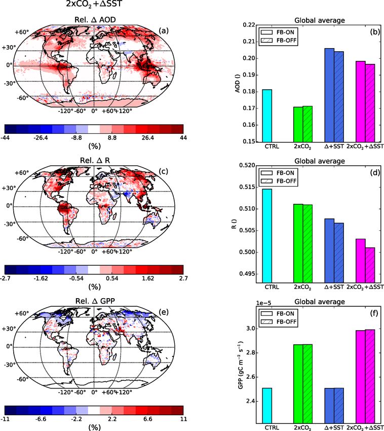
M. K. Sporre et al.: BVOC–aerosol–climate feedbacks investigated using NorESM                                            4765

effects, e.g. on methane lifetime and ozone concentrations,      munity Atmosphere Model (CAM). The atmospheric model
but these effects will not be investigated in this study.        in NorESM is therefore called CAM-Oslo (Kirkevåg et al.,
   Both measurement and modelling studies have previ-            2013). We used CAM5.3-Oslo (Kirkevåg et al., 2018) cou-
ously investigated parts of the BVOC feedback shown in           pled to the Community Land Model version 4.5 (CLM4.5)
Fig. 1. Using long-term data of aerosol properties from 11       (Oleson et al., 2013). CLM4.5 was run in the BGC (bio-
measurement stations, Paasonen et al. (2013) estimated the       geochemistry) mode, which includes active carbon and nitro-
feedback associated with the T loop to globally be about         gen biogeochemical cycling. In this mode, the plants respond
−0.01 W m2 K−1 . Scott et al. (2018a) found a similar num-       to changes in environmental conditions by enhanced or re-
ber (−0.013 W m2 K−1 ) using a global aerosol model to-          duced growth, but the geographical vegetation distribution
gether with an offline radiative transfer model. In Kulmala      does not change. Included in CLM4.5 is the Model of Emis-
et al. (2014), the T branch of the feedback was estimated with   sions of Gases and Aerosols from Nature (MEGAN) version
an atmospheric model by doubling monoterpene emissions.          2.1 (Guenther et al., 2012) that provides emissions of BVOC
This resulted in a global cloud radiative forcing of approxi-    from the plant functional types in CLM4.5. The BVOCs
mately −0.2 W m2 . Makkonen et al. (2012) found this num-        include isoprene and the following compounds which are
ber to be −0.5 W m2 at lower anthropogenic aerosol emis-         lumped together as monoterpenes in CAM-Oslo; myrcene,
sions, using emissions from 2100 according to RCP4.5. The        sabinene, limonene, 3-carene, t-B-ocimene, β-pinene, α-
GPP branch has been investigated using measurement data          pinene. Both the vegetation and the emissions respond to
from a station in central Finland, which supported a statis-     changes in diffuse radiation, CO2 and other climate variables.
tically significant correlation between an increase in diffuse   CO2 inhibition is included in MEGAN for isoprene (Guen-
radiation ratio and higher aerosol loading during cloud-free     ther et al., 2012).
conditions, as well as a resulting increase in GPP (Kulmala         The aerosol scheme in CAM5.3-Oslo is called OsloAero
et al., 2013, 2014). Rap et al. (2018) combined a global         (Kirkevåg et al., 2018) and has been developed at the Me-
aerosol model, a radiation model and a land surface scheme       teorological Institute of Norway and the University of Oslo.
and found the GPP branch to contribute with a gain in global     OsloAero can be described as a “production-tagged” aerosol
BVOC emissions by 1.07. To our knowledge, no study has so        scheme where the aerosol tracers are defined according to
far used an Earth system model to investigate both branches      their formation mechanism. The tracers include 15 lognor-
of the BVOC feedback.                                            mal background modes, which are modified by condensa-
   This study provides a comprehensive global investigation      tion, coagulation and cloud processing. CAM5.3-Oslo also
of the BVOC feedback using an Earth system model. The            includes some changes to the gas-phase chemistry compared
model setup enables the vegetation and emissions in the land     to CAM5.3. In CAM5.3-Oslo, isoprene and monoterpene can
model to respond to changes in climate, CO2 and radiation,       react with O3 , OH and NO3 . The reaction between monoter-
capturing diurnal as well as seasonal variations in the emis-    pene and O3 yields low volatile SOA (LVSOA), while the
sions of BVOCs. Both emissions of isoprene and monoter-          other five reactions between BVOCs and the oxidants yield
penes are calculated interactively by the land model and are     semi-volatile SOA (SVSOA). The yields for the isoprene re-
included in the SOA formation in the atmospheric model.          actions are 0.05 and the yields for the monoterpene reac-
The scientific objectives of the study are to investigate the    tions are 0.15, which reflects the findings in, e.g. Jokinen
impact of CO2 and temperature on the BVOC feedback sep-          et al. (2015). LVSOA and SVSOA can also be formed from
arately and combined. We aim to determine the importance         dimethyl sulfide as a proxy for methane sulfonic acid (MSA).
of each step along the BVOC-feedback loop globally and re-       Only the LVSOA takes part in the nucleation in the model,
gionally. Moreover, we want to determine the relative impor-     while the SVSOA condenses onto already formed aerosol
tance of the two branches of the feedback loop, as well as the   particles (Makkonen et al., 2014). In NorESM, both LVSOA
overall relevance of the BVOC-feedback loop for estimating       and SVSOA are treated as non-volatile with condensation be-
the future climate.                                              ing kinetically limited.
                                                                    The nucleation scheme was introduced into CAM-Oslo in
                                                                 Makkonen et al. (2014) but has since then been further de-
2     Method                                                     veloped (Kirkevåg et al., 2018). The nucleation scheme in-
                                                                 cludes binary homogeneous sulfuric acid–water nucleation
2.1    Model description                                         (Vehkamäki et al., 2002), as well as an activation-type nu-
                                                                 cleation in the boundary layer. The activation-type nucle-
In this study, the Norwegian Earth System Model (NorESM)         ation rate is calculated from the concentrations of H2 SO4
(Bentsen et al., 2013; Kirkevåg et al., 2013; Iversen et al.,    and LVSOA available for nucleation according to Eq. (18)
2013) has been used to investigate the feedback loop de-         (J = 6.1 × 10⁻⁷ [H2 SO4 ] + 0.39 × 10⁻⁷ [LVSOA]) from Paa-
scribed in the previous section. NorESM is based on the          sonen et al. (2010). The subsequent growth and survival to
Community Earth System Model (CESM) but uses a differ-           the smallest mode (median radius 23.6 nm) is modelled by
ent ocean model and a different aerosol module in the Com-       a parameterisation from Lehtinen et al. (2007), depending

www.atmos-chem-phys.net/19/4763/2019/                                            Atmos. Chem. Phys., 19, 4763–4782, 2019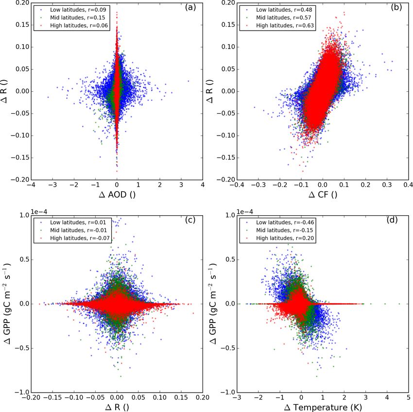
4766                                    M. K. Sporre et al.: BVOC–aerosol–climate feedbacks investigated using NorESM

mainly on the ratio between coagulation sink and growth rate       to enhanced CO2 concentrations. The CO2 was doubled with
(from LVSOA and H2 SO4 ). The treatment of early growth            respect to year 2000 level (denoted 2×CO2 ), but note that the
of aerosols has been adjusted in this version of the model         fixed SSTs highly restricted the temperature increase from
due to too-high concentrations of particles from new parti-        the radiative forcing associated with doubling the CO2 . The
cle formation. This was due to the survival percentage from        second experiment simulated the impact of a warmer cli-
nucleation (radius 2 nm) to the smallest mode being unrealis-      mate driven by a change in the sea surface temperature (SST)
tically high. In OsloAero, coagulation is calculated only be-      and sea ice to year 2080 conditions according to the RCP8.5
tween small modes and larger modes, while autocoagulation          scenario (denoted +1SST) but with fixed CO2 concentra-
and coagulation between smaller modes are considered neg-          tions at the year 2000. The year 2080 was chosen because
ligible. In order to improve this, we added coagulation onto       the CO2 levels at this time are approximately equal to the
all pre-existing particles to the coagulation sink used in the     2 × CO2 experiment. The temperature difference over land
survival calculation (Lehtinen et al., 2007).                      resulting from the increase in SST is shown in Fig. S1. In the
   The hygroscopicity of aerosol particles in NorESM is cal-       last experiment, we doubled both the CO2 and changed the
culated for each “mixture”, which is what the background           SSTs and sea ice as described previously (2 × CO2 +1SST).
modes are called after they have changed composition and           The experiments enable us to investigate the response of the
shape through condensation, coagulation and cloud process-         BVOC feedback to increased CO2 and temperature sepa-
ing. The hygroscopicity is a mass-weighted average of all          rately and then to see their combined effect in the last exper-
components in the mixtures if the particles are uncoated           iment. Because the aerosol loading is expected to decrease
or have thin coating. If the particles have a thick coating        in the future (Smith et al., 2016), we also ran a simulation
(> 2 nm), the hygroscopicity is instead a mass-weighted av-        identical to the 2 × CO2 +1SST but where we changed the
erage of the coating itself (Kirkevåg et al., 2018). Both the      emissions of aerosol and precursor gases to PI levels (1850),
size and hygroscopicity of the aerosol particles are used in       denoted 2 × CO2 +1SST LA (low aerosol). This simulation
the calculations of CCN and the activation of aerosols to          was done in order to investigate whether the importance of
cloud droplets.                                                    the BVOC feedback will be larger if the aerosol loading is
   The cloud schemes in CAM5.3-Oslo include a deep con-            smaller in the future. The doubling of CO2 , the SST increase
vection scheme (Zhang and McFarlane, 1995), a shallow              and the reduction in aerosol emissions are all at the top end of
convection scheme (Park and Bretherton, 2009) and the mi-          possible future scenarios and are not the most likely future.
crophysical two-moment scheme MG1.5 (Morrison and Get-                To be able to determine the importance of each step along
telman, 2008; Gettelman and Morrison, 2015) for stratiform         the BVOC-feedback loop, each of the experiments described
clouds. The microphysical scheme includes aerosol activa-          were run with the feedback loop turned on (FB-ON) and
tion according to Abdul-Razzak and Ghan (2000), which de-          turned off (FB-OFF). In the FB-OFF simulations, we did
pends on updraft velocity and the properties of the different      not want changes in CO2 , temperature or GPP to affect the
aerosol modes. For both liquid and ice, the mass and number        BVOC emissions, essentially keeping concentrations con-
are prognostic and the autoconversion scheme (Khairoutdi-          stant at present-day (PD) levels. This was done by gener-
nov and Kogan, 2000) includes subgrid variability of cloud         ating emission fields from a control simulation and using
water (Morrison and Gettelman, 2008). In this paper, the           these as input into the FB-OFF simulations; see Fig. 2 and
methods from Ghan (2013) are used to calculate the forcing         Table 1. We found that reproducing the diurnal variations in
from clouds and aerosols. The net direct forcing (NDFGhan )        the BVOC emissions in the FB-OFF simulations was impor-
is calculated as the difference between the net top-of-the-        tant in order to get the BVOC concentrations in the model
atmosphere radiative flux and the radiative flux, neglect-         representative of those in the control simulation. The col-
ing the scattering and absorption of solar radiation by the        umn burdens of isoprene and monoterpene became much
aerosols (Fclean ). This is calculated in a separate call to the   higher when no diurnal variation in the BVOC emissions was
radiation code. Similarly, the net cloud forcing (NCFGhan )        included, since the BVOC emissions were high also when
is calculated as the difference between Fclean and the flux        the oxidant concentrations were low. Moreover, the reaction
neglecting the scattering and absorption by both clouds and        rates between the BVOCs and the oxidants are temperature
aerosols (Fclear,clean ). In the model, the forcings are calcu-    dependent and thus lower during the nights. In order to pro-
lated separately for the short-wave and long-wave radiation,       duce emission fields for the FB-OFF simulations with correct
which we have used to calculate the net forcing.                   diurnal variations, 6 years of control run emission data at half
                                                                   an hour time resolution were averaged to create a yearly in-
2.2    Experimental setup                                          put file with half an hour time resolution (the time step used
                                                                   in the model). Thus, the FB-ON simulations and the FB-
In order to investigate the feedback loop presented above,         OFF simulations are set up exactly the same way, except that
three different sets of experiments were performed with            the FB-ON simulations are run with interactive BVOC emis-
NorESM. The first experiment was set up to simulate im-            sions, while in the FB-OFF simulations the BVOC emissions
pacts of the change in BVOC emissions when plants respond          are fixed at PD conditions; see Table 1.

Atmos. Chem. Phys., 19, 4763–4782, 2019                                             www.atmos-chem-phys.net/19/4763/2019/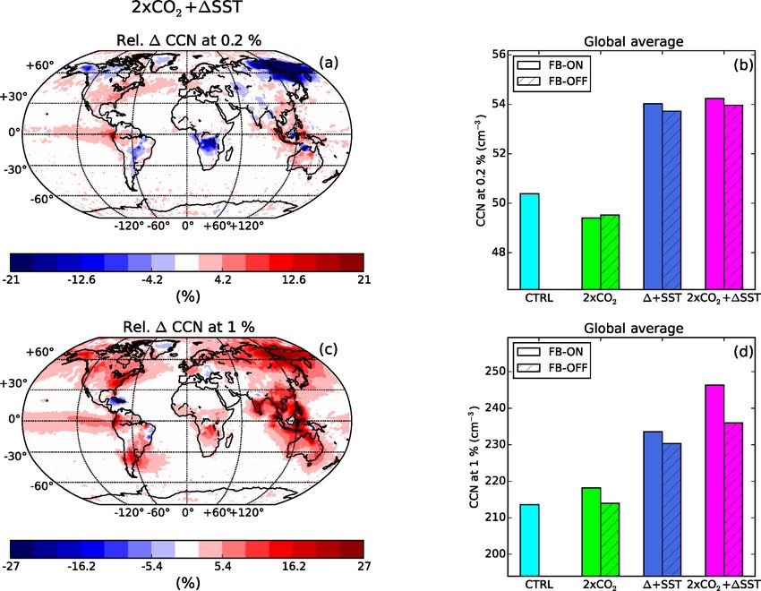
M. K. Sporre et al.: BVOC–aerosol–climate feedbacks investigated using NorESM                                                   4767

Table 1. Specifications of the CO2 levels, year of the SSTs, BVOC emissions and which meteorology was used for the nudging for each of
the simulations. “Met” stands for meteorology and refers to the simulations denoted by met in Fig. 2.

  Experiment                       CO2         SSTs and sea ice     BVOC emissions     Aerosol emissions   Meteorology
  CTRL                             1 × CO2     PD                   Interactive               PD           CTRL met
  2 × CO2 FB ON                    2 × CO2     PD                   Interactive               PD           2 × CO2 met
  2 × CO2 FB OFF                   2 × CO2     PD                   Fixed (CTRL)              PD           2 × CO2 met
  +1SST FB ON                      1 × CO2     2080                 Interactive               PD           +1SST met
  +1SST FB OFF                     1 × CO2     2080                 Fixed (CTRL)              PD           +1SST met
  2 × CO2 +1SST FB ON              2 × CO2     2080                 Interactive               PD           2 × CO2 +1SST met
  2 × CO2 +1SST FB OFF             2 × CO2     2080                 Fixed (CTRL)              PD           2 × CO2 ,+1SST met
  2 × CO2 +1SST FB ON LA           2 × CO2     2080                 Interactive               PI           2 × CO2 +1SST met LA
  2 × CO2 +1SST FB OFF LA          2 × CO2     2080                 Fixed (CTRL)              PI           2 × CO2 +1SST met LA

                                                                       experiment are nudged to separate NorESM runs with the
                                                                       corresponding temperature/CO2 changes (see Fig. 2 and Ta-
                                                                       ble 1). The nudging changes some of the meteorological vari-
                                                                       ables in the model slightly and therefore also the control sim-
                                                                       ulation (CTRL), from which the fixed BVOC emission fields
                                                                       are generated, was nudged to another CTRL simulation (see
                                                                       Fig. 2).
                                                                          NorESM was run with a 1.9 × 2.5◦ horizontal resolution,
                                                                       30 vertical levels and fixed sea ice and SSTs. The emissions
                                                                       of aerosols and precursor gases were set to the year 2000, ex-
                                                                       cept for the simulations where we decrease the aerosol load-
                                                                       ing to PI levels, where the emissions from 1850 are used. Pre-
                                                                       scribed oxidant fields and land use at PD conditions are used
                                                                       for all simulations. CTRL and the other four experiments de-
                                                                       scribed above were run for 30 years as a spin-up (see Fig. 2).
                                                                       After this, another 8 years were run to create the meteorolog-
                                                                       ical data for nudging for each experiment. The FB-ON simu-
                                                                       lations were initialised from the spin-up simulations and run
                                                                       for 8 years using nudging with a relaxation time of 6 h. The
                                                                       FB-OFF simulations were run in the same manner, except
                                                                       that the BVOC emissions were read from file (as described
                                                                       above). The first 2 years of the FB-ON and FB-OFF simu-
Figure 2. The simulation setup. The CTRL simulation has CO2 and
                                                                       lations are considered a spin-up, due to the nudging and the
SSTs at present-day (PD) levels. The 2×CO2 simulations have dou-
                                                                       change in the emissions in the FB-OFF simulations. Thus,
bled CO2 with respect to the year 2000. In the +1SST simulations,
the SST and sea ice are increased to the year 2080 levels. In the      the last 6 years of the simulations are used for the analysis.
2 × CO2 +1SST simulation, the CO2 is doubled and the SST and
sea ice are changed to the year 2080 levels. The CTRL, as well as
all FB-ON and FB-OFF simulations, is nudged to their respective        3     Results and discussions
met simulation. All FB-ON simulations have interactive emissions,
while the FB-OFF simulations have fixed emissions from the CTRL        3.1     BVOC emissions and SOA
simulation.
                                                                       We will start by discussing the part of the BVOC feedback
                                                                       common to the two branches and then discuss each branch of
                                                                       the feedback separately.
   Furthermore, to not have changes in weather patterns be-
tween the FB-ON and FB-OFF simulations mask the effects                3.1.1    BVOC emissions
of the different BVOC emissions, we have used nudging
(Kooperman et al., 2012) of horizontal winds and surface               The BVOC emissions calculated by NorESM are in line
pressure (Zhang et al., 2014). Since meteorological condi-             with previous studies. In the CTRL run, the BVOC emis-
tions change significantly with doubling of CO2 and tem-               sions are 366 Tg yr−1 for isoprene and 115 Tg yr−1 for
perature increase, the FB-ON/FB-OFF simulations for each               monoterpenes. These values are in the range of those in

www.atmos-chem-phys.net/19/4763/2019/                                                   Atmos. Chem. Phys., 19, 4763–4782, 2019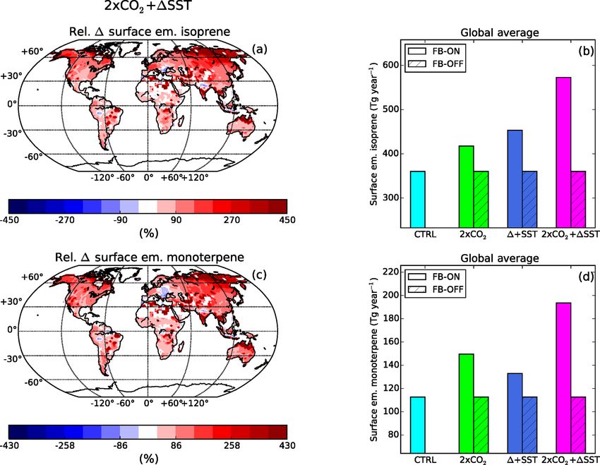
4768                                     M. K. Sporre et al.: BVOC–aerosol–climate feedbacks investigated using NorESM

Figure 3. The relative difference between the FB-ON and FB-OFF simulations of the annual average surface emissions of isoprene (a) and
monoterpenes (c) for the 2 × CO2 +1SST experiment. The relative difference is defined as the (FB-ON − FB-OFF) / FB-OFF. In the bar
plots, the yearly global surface emissions of isoprene (b) and monoterpenes (d) for the CTRL simulation as well as the three experiments
(both FB-ON and FB-OFF simulations) are shown.

Guenther et al. (2012) for monoterpenes but on the lower              in the tropics (parts of Africa and the Amazon), especially
end for isoprene. For the 2 × CO2 +1SST FB-ON simula-                 in the +1SST experiment, both monoterpene and isoprene
tion, the emissions are 586 Tg yr−1 (+60 %) for isoprene and          emissions decrease. This is caused by a decrease in the LAI
198 Tg yr−1 (+73 %) for monoterpenes. The emissions are               associated with plant mortality that seems to occur because
somewhat lower than estimated for the future climate in pre-          of heat stress. The decrease in LAI leads to a lower albedo
vious studies (Laothawornkitkul et al., 2009) but the rela-           in these forest regions, which further increases the tempera-
tive increases are on the high end (Carslaw et al., 2010). The        ture, causing more heat stress and creating a feedback mecha-
isoprene emissions increase more when the temperature is              nism on the vegetation. Nevertheless, the vegetation has had
increased (+1SST) than when the CO2 is doubled, but the               time to adapt to the new temperatures and stabilise by the
opposite is true for monoterpenes; see Fig. 3c and d.                 end of the 30-year spin-up period. The decreases in LAI are
   The emissions of isoprene and monoterpenes are higher              smaller in the 2×CO2 +1SST experiments as the vegetation
almost everywhere in the FB-ON simulations with 2 × CO2 ,             is seeded by CO2 (Fig. 3a).
+1SST and 2 × CO2 +1SST than in the FB-OFF simula-
tions with the same setup (see Figs. 3 and S2), in line with          3.1.2   SOA
the BVOC feedback. The absolute increase in the emissions
is largest over the tropical forests, while the relative increase
                                                                      The higher BVOC emissions in the FB-ON simulations lead
in emissions is greatest over the boreal forests in the Northern
                                                                      to larger SOA production (see Fig. 4b), as expected from the
Hemisphere (NH). Generally, the CO2 inhibition of isoprene
                                                                      BVOC feedback. The SOA production in the CTRL simu-
is masked by the CO2 and temperature boosts of the vegeta-
                                                                      lation is 75 Tg yr−1 , which is in the range previously esti-
tion, which leads to a higher leaf area index (LAI) and GPP.
                                                                      mated by global models (Tsigaridis et al., 2014; Glasius and
In the experiment with only increased CO2 , there are a few
                                                                      Goldstein, 2016). The SOA production in the FB-ON sim-
areas in Africa and India that seem to have lower isoprene
                                                                      ulations is similar for the 2 × CO2 and +1SST experiments
emissions due to CO2 inhibition. This can be seen as lower
                                                                      (90 and 92 Tg yr−1 ) while the combined effect of higher CO2
isoprene emissions and higher monoterpene emissions in the
                                                                      and temperature gives a higher SOA production, with values
same place (Fig. S2a and c). This does not occur in the exper-
                                                                      of 115 Tg yr−1 . The column burden of SOA is higher over
iments where also the SSTs are increased. Over some regions
                                                                      the entire globe when the BVOC feedback is on compared to

Atmos. Chem. Phys., 19, 4763–4782, 2019                                                 www.atmos-chem-phys.net/19/4763/2019/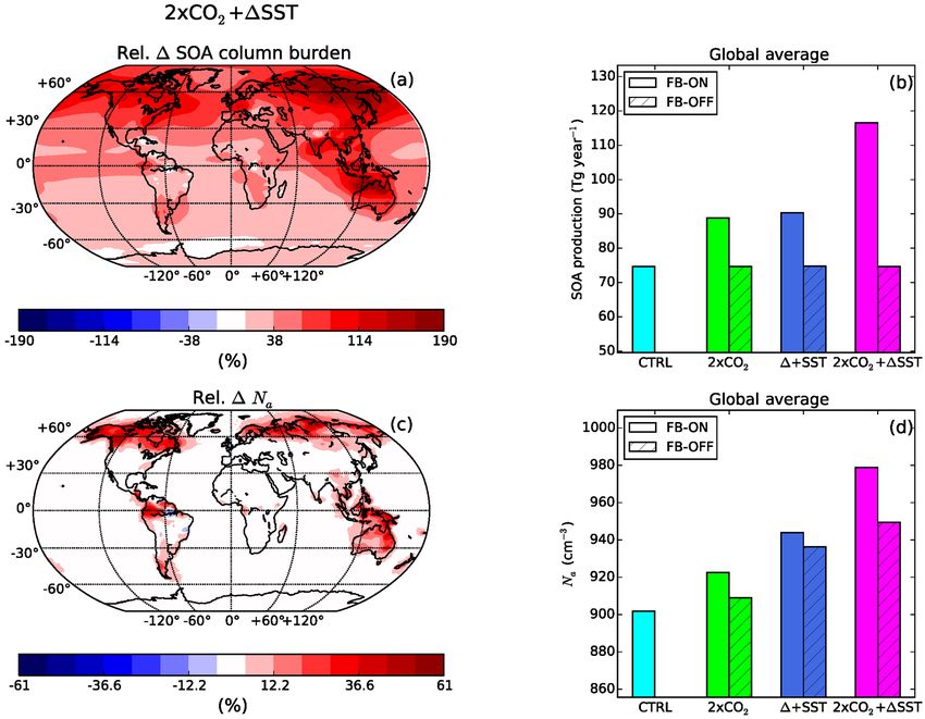
M. K. Sporre et al.: BVOC–aerosol–climate feedbacks investigated using NorESM                                                  4769

Figure 4. The relative difference between the FB-ON and FB-OFF simulations in the annual average column burden SOA (a) and Na in the
boundary layer (c) for the 2 × CO2 +1SST experiment. In the bar plots, the average yearly global production of SOA (b) and the global
average Na in the boundary layer (d) are shown for the CTRL simulation as well as the three experiments (both FB-ON and FB-OFF
simulations).

when it is turned off, except in the +1SST experiment over              In order to investigate the effect on the sizes of the par-
and downwind of the regions where the BVOC emissions de-             ticles, we analysed the averaged boundary layer aerosol size
crease; see Figs. 4a and S3b. The largest absolute increase of       distributions for two of the regions most affected by the feed-
column burden SOA is over the tropical forests, while the            back: the boreal forests and the tropical islands in southeast
largest relative increases are over the Arctic and sub-Arctic.       Asia. The size distributions are created from the number me-
The fraction of SOA in the aerosol particles is also higher          dian radius and standard deviations of the 12 particle mix-
when the feedback is turned on, which leads to a reduction in        tures in OsloAero (Kirkevåg et al., 2018). Over the boreal
the hygroscopicity of the particles (not shown).                     forests, the higher BVOC emissions result in more particles
                                                                     in the Aitken mode (Fig. 5a and b). The enhanced growth of
3.1.3   Aerosol number and size                                      the particles also results in more particles in the accumula-
                                                                     tion mode and in a shift to larger sizes of the Aitken mode,
Not only is the mass of the aerosol particles affected by            which results in a small decrease in the number of particles
higher levels of BVOCs but also the number concentration             below 25 nm. In the tropics, there is a larger (smaller) ab-
of aerosol particles and their sizes. The changes in the num-        solute (relative) increase in Aitken-mode particles. The shift
ber concentration and size of the particles vary with region.        in the size distribution due to more condensing vapours is
The largest difference in Na between the FB-ON and FB-               larger here than over the boreal forests and results in decreas-
OFF simulations occurs over, and downwind of, the tropi-             ing particle concentrations up to 70 nm. The biggest changes
cal rain forests, as well as over the boreal forests in the NH       in both number and shift in size distribution are seen in the
(see Fig. 4c). The relative difference is largest over the bo-       2 × CO2 +1SST experiment. The changes in particle sizes
real forests in the NH where the particle number concentra-          occur further downwind from the sources than the changes
tions are generally low. The largest absolute differences on         in aerosol number concentrations which are more restricted
the other hand occur in the tropics. Over regions where the          to areas close to the sources, in particular in the tropics.
emissions decrease (in the +1SST experiment), the Na de-
creases (Fig. S3d).

www.atmos-chem-phys.net/19/4763/2019/                                                 Atmos. Chem. Phys., 19, 4763–4782, 2019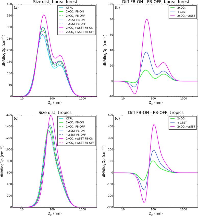
4770                                       M. K. Sporre et al.: BVOC–aerosol–climate feedbacks investigated using NorESM

Figure 5. Annually averaged aerosol number size distributions in the boundary layer for the boreal forest region (lat.: 55 to 70◦ N, long.:
180◦ W to 180◦ E) and the region around the tropical islands in southeast Asia (lat.: 20◦ S to 20◦ N, long.: 90–130◦ E). In panels (a) and (c),
the distributions from the CTRL and the three experiments are plotted, while in panels (b) and (d), the differences between the FB-ON and
FB-OFF simulations are plotted.

3.2     The T-feedback branch                                             low and the absolute decrease in CCN is small. Moreover,
                                                                          it should be noted that the CCN concentration in the model
3.2.1    CCN                                                              is calculated only for the cloud-free areas in the grid boxes.
                                                                          Thus, the particles that are activated into cloud droplets are
The CCN response of the feedback is a combination of the                  not included in the CCN concentrations. At higher supersatu-
changes in Na , particle sizes and hygroscopicity. The CCN                rations (1 %), also particles at smaller sizes can be activated,
concentrations are generally higher when the feedback is                  and thus the feedback results in more CCN almost every-
turned on, as is expected from the feedback (Fig. 1). How-                where (Fig. 6c). The areas downwind of the tropics, where
ever, at low supersaturations (0.2 %), the CCN concentra-                 the feedback mainly results in an increase in particle size,
tion over some regions (in particular over the boreal forests),           have higher CCN at both levels of supersaturation. The ef-
is lower in the simulations with the feedback turned on                   fect of increasing particle sizes and number generally domi-
(Fig. 6a). The cause for this is the large amount of Aitken-              nates the effect of decreased particle hygroscopicity since the
mode particles formed through new particle formation. The                 feedback contributes with increasing number of CCN.
smaller particles compete with the larger particles for the
water vapour, which reduces the number of aerosol parti-
cles that can activate into cloud droplets at low supersatu-
rations. The concentrations of CCN in these regions are very

Atmos. Chem. Phys., 19, 4763–4782, 2019                                                      www.atmos-chem-phys.net/19/4763/2019/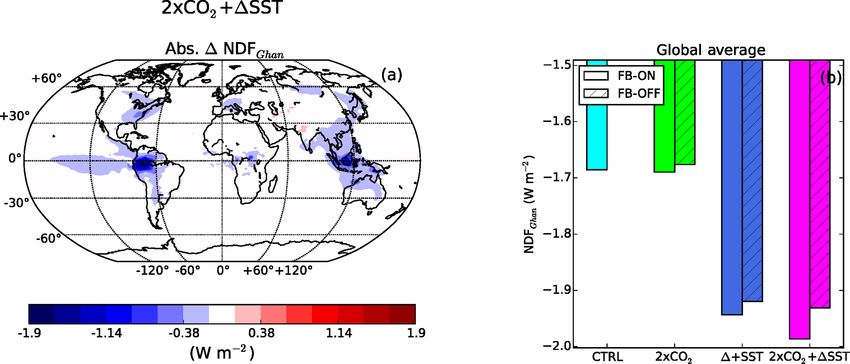
M. K. Sporre et al.: BVOC–aerosol–climate feedbacks investigated using NorESM                                                   4771

Figure 6. The relative difference between the FB-ON and FB-OFF simulations in the annual average CCN at 0.2 % (a) and 1 % (c) in the
boundary layer, for the 2 × CO2 +1SST experiment. In the bar plots, the globally averaged CCN at 0.2 % (b) and 1 % (d) in the boundary
layer are shown for the CTRL simulation as well as the three experiments (both FB-ON and FB-OFF simulations).

3.2.2   Cloud properties                                                The strongest and most widespread difference in the cloud
                                                                     microphysical effects occurs in the NH midlatitudes and high
                                                                     latitudes. One cause for this is the cloud cover and cloud
The effect from the BVOC feedback on the clouds is mainly            types present close to the emission regions. The clouds in
seen over and downwind of the regions where the BVOC                 the midlatitudes and high latitudes are commonly stratiform,
emissions change the most. The vertically averaged CDNC              for which the model includes Na in the calculations of CDNC
generally increase (as is expected from the BVOC feedback),          (through the Abdul-Razzak and Ghan, 2000 scheme for ac-
mainly north of 45◦ N and in the tropics Fig. 7a. The weakest        tivation). The differences in CDNC are not as widespread
response of the CDNC to the feedback occurs in the experi-           in the tropics, since shallow and deep convection (which
ment where only CO2 has been changed (Figs. 7b and S5). In           aerosols generally do not affect in ESMs) are the dominant
the experiment with only increased SST, the CDNC is higher           cloud types here. Another cause for the more widespread
mainly in the Northern Hemisphere since the BVOC emis-               cloud changes in the NH is the larger land areas here, i.e.
sions in parts of the tropics decrease (Fig. S5b). The higher        larger areas where the emissions differ.
levels of CDNC occur predominantly during the local sum-
mer when the BVOC emissions are the highest.                         3.2.3   Cloud forcing
   The increasing CDNC associated with the feedback is ac-
companied by a decrease in cloud droplet effective radius (re )      The potential of the BVOC feedback to affect future climate
and an increasing cloud water path (CWP) (Fig. 7c and e).            will now be evaluated by investigating the changes in cloud
The total cloud fraction (CF) does however not seem to be            forcing between the FB-ON and FB-OFF simulations. Since
impacted to the same extent (see Fig. 7g and h), which may           we cannot determine the full temperature response of the
be an effect of the nudging. There is an increase in the CF          feedback, the differences in forcing between the FB-ON and
over the boreal forests, mainly during winter, by up to 4 %.         FB-OFF simulations will be used to estimate the potential
In summer, there is an increase in low- and mid-level clouds         climate impact of the changed cloud properties. The patterns
over the Arctic and NH midlatitudes. This is accompanied             of the difference in the cloud forcing between the simulations
by a decrease in the high-level clouds and therefore does not        with the FB turned on and the FB turned off (Fig. 8a and c)
show up clearly in Fig. 7g. In the tropics, there are no system-     resemble the patterns of the difference in CDNC (Fig. 7a).
atic changes in the cloud fraction as a result of the feedback.      The higher CDNC in the high latitudes and midlatitudes as-

www.atmos-chem-phys.net/19/4763/2019/                                                  Atmos. Chem. Phys., 19, 4763–4782, 2019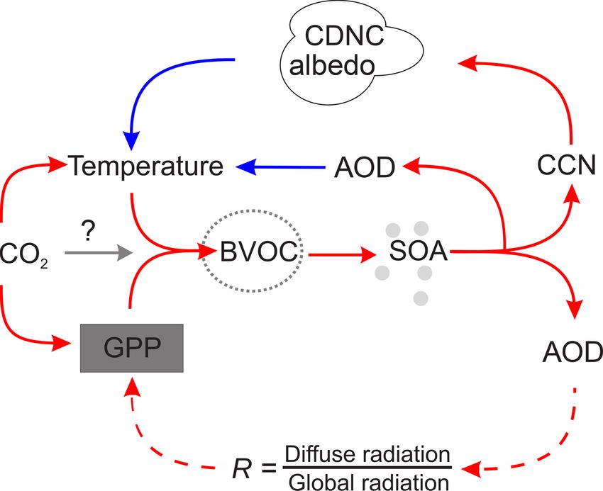
4772                                      M. K. Sporre et al.: BVOC–aerosol–climate feedbacks investigated using NorESM

Figure 7. The relative/absolute difference between the FB-ON and FB-OFF simulations in the annual vertically averaged CDNC (a), the
vertically averaged re (c), the CWP (e) and the total CF (g) for the 2 × CO2 +1SST experiment. In the bar plots (b, d, f, h), the globally
averaged values of the same variables are shown for the CTRL simulation as well as the three experiments (both FB-ON and FB-OFF
simulations). For the CDNC, re and CWP, the in-cloud values are used.

sociated with the FB is accompanied by a decrease in the                  The feedback does not only contribute with an enhanced
NCFGhan by up to −11 W m−2 during the 3 summer months;                 negative cloud forcing though. The difference in NCF at the
see Fig. 8a. The effect of the feedback is seen mainly during          surface (1 NCFS ) between the FB-ON and FB-OFF simula-
the local summer when the BVOC emissions are the high-                 tions is positive over the NH boreal forests during winter in
est. The differences in NCFGhan are smallest in the 2 × CO2            the experiments with increased SST (Figs. 8e and S6f). The
experiment and strongest in the 2 × CO2 +1SST experiment               changes in microphysical properties as well as cloud cover
(Figs. 8 and S6).                                                      lead to an increase in the positive long-wave cloud forcing

Atmos. Chem. Phys., 19, 4763–4782, 2019                                                  www.atmos-chem-phys.net/19/4763/2019/
M. K. Sporre et al.: BVOC–aerosol–climate feedbacks investigated using NorESM                                                         4773

Figure 8. The absolute difference between the FB-ON and FB-OFF simulations for the NCFGhan during June, July and August (a), December
January and February (c), as well as the NCFS during December, January and February (e) for the 2 × CO2 +1SST experiment. In the bar
plots (b, d, f), the globally averaged values of the same variables are shown for the CTRL simulation as well as the three experiments (both
FB-ON and FB-OFF simulations).

(LWCF) at the surface, which is larger than the correspond-             BVOC feedback in the Arctic during summer could possibly
ing increase in negative short-wave cloud forcing (SWCF).               counteract part of this Arctic amplification. The large im-
It can be concluded that the BVOC feedback can contribute               pact of the feedback in the NH midlatitudes and high lat-
to both enhanced and reduced negative cloud forcing de-                 itudes also results in a quite large difference in the effect
pending on region and season. Nevertheless, the difference in           of the feedback between the hemispheres. The difference in
yearly global average NCFGhan is −0.43 W m−2 (SWCFGhan                  the NCFGhan , between the FB-ON and FB-OFF simulations
−0.45 W m−2 , LWCFGhan 0.02 W m−2 ) between the FB-ON                   for the 2 × CO2 +1SST experiments, is −0.56 W m−2 in the
and FB-OFF simulations in the 2×CO2 +1SST experiment,                   NH, while in the SH it is −0.30 W m−2 .
indicating that the feedback can contribute with a potentially
important impact on the future climate on a global scale.               3.3     The GPP-feedback branch
   The strongest and most widespread negative cloud forc-
ing associated with the feedback is seen in the Arctic dur-             3.3.1    AOD
ing summer. This is interesting since the Arctic is currently,
                                                                        The higher aerosol loading associated with the feedback also
and is expected to continue, experiencing the largest warm-
                                                                        results in higher values for the aerosol optical depth (AOD),
ing in response to the increasing atmospheric concentrations
                                                                        in line with the feedback in Fig. 1. The largest relative dif-
of greenhouse gases (IPCC, 2013). The strong impact of the
                                                                        ferences between the FB-ON and FB-OFF simulations oc-

www.atmos-chem-phys.net/19/4763/2019/                                                      Atmos. Chem. Phys., 19, 4763–4782, 2019
4774 M. K. Sporre et al.: BVOC–aerosol–climate feedbacks investigated using NorESM
Figure 9. The relative difference between the FB-ON and FB-OFF simulations in the annually average AOD (a), R (c) and GPP (e) for the
2 × CO2 +1SST experiment. In the bar plots (b, d, f), the globally averaged values of the same variables are shown for the CTRL simulation
as well as the three experiments (both FB-ON and FB-OFF simulations).
cur over, and downwind of, the tropical forest and the boreal ference in total cloud cover (0.53) is higher than between
forests in the NH; see Fig. 9a. The AOD effects are largest in the difference in R and the difference in AOD (0.08); see
the local summer when the emissions are the highest. Fig. 10a and b. Small changes in the cloud cover can offset
the AOD effects on R. Changes in cloud cover can therefore
3.3.2 Diffuse radiation explain the decreases in R over, e.g. Scandinavia (Fig. 9),
even though the AOD increases there. The increase in R is
expected from the BVOC feedback but the larger dependency
The ratio between the diffuse radiation and the global radia-
in R on cloud fraction than AOD was not expected.
tion is, according the BVOC-feedback hypotheses, expected
to increase with higher aerosol scattering. Our model simu-
lations show only a small relative difference in R (maximum 3.3.3 GPP
5 %) between the FB-ON and FB-OFF simulations (Fig. 9c).
The regions where there is a strong difference in R between Next, we will investigate the relationship between R and
the FB-ON and FB-OFF simulations correspond to the re- GPP. Neither in the maps nor in the statistical analyses do we
gions with the largest change in AOD. However, a statistical find any strong relationship between R and GPP; see Figs. 9e
analysis of the differences between the monthly means from and 10c. The positive effect of diffuse radiation on vegetation
the FB-ON and FB-OFF simulations shows that the corre- growth is included in CLM (Oleson et al., 2013) but it seems
lation coefficient between the difference in R and the dif- like other factors perturbed by the T branch are affecting the
Atmos. Chem. Phys., 19, 4763–4782, 2019 www.atmos-chem-phys.net/19/4763/2019/M. K. Sporre et al.: BVOC–aerosol–climate feedbacks investigated using NorESM 4775 Figure 10. Scatter plots of the absolute differences (FB-ON − FB-OFF) in AOD and R in panel (a), CF and R in panel (b), GPP and R in panel (c) and GPP and temperature in the lowest model layer in panel (d). Data from all three experiments (2 × CO2 , +1SST and 2 × CO2 +1SST) are included. Each dot is a monthly average for one grid box. Only grid boxes with a land fraction of 1 and GPP greater than zero are included. The dots are coloured according to latitude bands (high latitudes: 90–55◦ S and 55–90◦ N, midlatitudes: 55–30◦ S and 30–55◦ N, low latitudes: 30◦ S–30◦ N) and the correlations coefficient r for each region is shown in the legend. Based on the model output, AOD does not drive diffuse radiation fraction, but cloud fraction does; and diffuse radiation does not drive gross primary product, but temperature does. vegetation more. Moreover, the difference in R between the associated with lower temperatures caused by the enhanced FB-ON and FB-OFF simulations was quite small. The rela- negative NCFGhan . Even though we are running with fixed tionship between R and GPP is also affected by changes in SSTs, the temperatures over land can change somewhat in re- the total amount of radiation. If the total radiation decreases sponse to the changed forcing. In addition, a decrease in total sufficiently, an increase in R will not boost GPP (Knohl and visible radiation reaching the vegetation, associated with the Baldocchi, 2008). There is a negative correlation between the increase in low-cloud cover in this region, can contribute to change in R and the change in the total visible radiation in the decrease in GPP. Overall, the GPP is slightly lower in the our experiments, and the total visible radiation is generally simulations where we include the feedback, which is oppo- lower in the feedback on simulations (see Fig. S8a). The hy- site to what is expected from the feedback in Fig. 1. These re- pothesised boost of GPP by R might therefore be masked by sults are in contrast to the results by Rap et al. (2018), which the change in the total visible radiation. Since the focus of did not include the effects from the T branch in their study. In this study is the effect of the feedback on a global scale, we our study, it seems that the effects from the T branch of the have chosen not to look into if we can find the effect of R on BVOC-feedback loop is dominating over the GPP branch. GPP in certain conditions or locations. The GPP branch may however be important on local scales The GPP instead seems to respond to changes associated ot resolvable by NorESM. with the T-feedback branch (Fig. 10d). In particular, there is a decrease of GPP in the sub-Arctic during the summer months www.atmos-chem-phys.net/19/4763/2019/ Atmos. Chem. Phys., 19, 4763–4782, 2019
4776                                     M. K. Sporre et al.: BVOC–aerosol–climate feedbacks investigated using NorESM

Figure 11. The absolute difference between the FB-ON and FB-OFF simulations in the annual average NDFGhan (a) for the 2×CO2 +1SST
experiment. In panel (b), the globally averaged NDFGhan for the CTRL simulation as well as the three experiments (both FB-ON and FB-OFF
simulations) are shown.

3.4    Direct aerosol forcing                                         Table 2. Difference in the global annual average NCFGhan ,
                                                                      NDFGhan and total aerosol forcing (TAFGhan ) between the FB-ON
The scattering of radiation from aerosols in the atmosphere           and FB-OFF simulations.
did not seem to impact the GPP significantly in our experi-
                                                                                              1NCFGhan      1NDFGhan      1TAFGhan
ments, but we do find a direct impact on climate. The annual
                                                                       Experiments             (W m−2 )      (W m−2 )      (W m−2 )
average NDFGhan is locally down to −2.2 W m−2 when the
feedback is turned on; see Fig. 11a. The largest differences           2 × CO2                     −0.11        −0.014         −0.12
in NDFGhan between the FB-ON and FB-OFF simulations is                 +1SST                       −0.19        −0.025         −0.22
seen close to the sources and over the regions that have large         2 × CO2 +1SST               −0.43        −0.058         −0.49
                                                                       2 × CO2 +1SST LA            −0.66        −0.074         −0.73
absolute changes in the emissions, i.e. the tropics. Globally
averaged, the difference in NDFGhan is −0.06 W m−2 for the
2 × CO2 +1SST experiment. This is approximately 15 % of
the difference in forcing from the clouds. The magnitude of           the effects on the clouds are largest in the 2 × CO2 +1SST
the differences in the NDFGhan indicates that the BVOC feed-          LA experiment is not surprising, since clouds formed in
back can provide an, at least regionally, enhanced negative           clean condition are most susceptible to aerosol perturbations
forcing also through the direct aerosol forcing.                      (Spracklen and Rap, 2013).
                                                                         The stronger BVOC impact on the clouds in the exper-
3.5    Future lower aerosol loading                                   iment with lower aerosol loading result in a larger impact
                                                                      from the feedback on the radiation budget. The difference in
In order to investigate how the impact of the feedback                the yearly global average NCFGhan for the 2 × CO2 +1SST
changes if the aerosol emissions decrease in the future,              LA is 53 % higher than for the 2 × CO2 +1SST experi-
we also ran the 2 × CO2 +1SST experiment with lower                   ment; see Table 2. In addition, the direct effect associated
anthropogenic aerosol emissions. The BVOC emissions in                with the feedback is larger when the anthropogenic aerosol
2 × CO2 +1SST LA FB-ON simulation are almost the same                 load is reduced. The difference in NDFGhan is 29 % higher
as those in the 2 × CO2 +1SST FB-ON simulation (4 %                   for the experiment with lower aerosol loading. These results
and 3 % higher for isoprene and monoterpenes). The re-                show that the importance of the BVOC feedback will be-
sponse to the feedback is however larger in the experiment            come substantially greater if, as expected, the anthropogenic
with lower anthropogenic emissions. The relative differences          aerosol emissions are reduced in the future. These results
in Na are larger, especially over regions with large anthro-          are interesting, especially since some large emitters have al-
pogenic emissions in PD. This indicates that BVOCs will               ready started reducing their SO2 emissions (Li et al., 2017).
be more important for aerosol formation in the future, if the         The total aerosol forcing associated with the feedback in the
anthropogenic emissions decrease. The relative CDNC dif-              2 × CO2 +1SST (LA) experiment is −0.49 (−0.73) W m−2 ,
ference is also greater in the experiment with low anthro-            which is 13 (20) % of the positive radiative forcing (calcu-
pogenic emissions in both the tropics and the NH. There are           lated according to Myhre et al., 1998) associated with a sim-
areas (such as southeast Asia) where the relative differences         ilar doubling of CO2 .
in CDNC are close to zero in the 2×CO2 +1SST experiment
and up to 30 % in the 2 × CO2 +1SST LA experiment. That

Atmos. Chem. Phys., 19, 4763–4782, 2019                                                 www.atmos-chem-phys.net/19/4763/2019/
M. K. Sporre et al.: BVOC–aerosol–climate feedbacks investigated using NorESM 4777
3.6 Limitations and uncertainties in region and level where the SOA formation occurs. This
has been shown to affect the indirect aerosol effect (Karset
The investigation of the effects of BVOCs is challenging et al., 2018). Monthly BVOC emission files should there-
since it involves complex interactions not only in the atmo- fore be used with caution. In this study, prescribed oxidant
sphere but also in the biosphere. In this investigation, the fields at PD conditions with applied diurnal variation for OH
focus has been on the potential atmospheric consequences and HO2 were used. Running the model with more advanced
of increased BVOC emissions. However, the future BVOC gas-phase chemistry would have simulated the interactions
emissions are highly sensitive to what will happen to the between the BVOCs and the oxidants more realistically.
vegetation. This was clearly seen in our simulations where New particle formation, BVOC and SOA parameterisa-
we increased only the SST and found that GPP is reduced tions are now implemented in many ESMs but are still un-
in several regions due to heat stress. This cancels or even der development and associated with uncertainties (e.g. Tsi-
reverses the BVOC feedback in these regions. How future garidis and Kanakidou, 2018; Makkonen et al., 2014; Gor-
vegetation will respond to climate change is still highly un- don et al., 2016). The BVOC feedback mechanism is highly
certain (Friend et al., 2014). sensitive to the parameterisations associated with new parti-
Our simulations do not allow changes in the distribution cle and SOA formation. The yields associated with the for-
of the vegetation and therefore do not include any effects mation of LVSOA and SVSOA from monoterpenes and iso-
of geographical shifts in vegetation. A poleward shift in the prene are largely uncertain, which may significantly affect
vegetation could increase the BVOC emissions in these re- the feedback. The parameterisations of nucleation rates and
gions (Peñuelas and Staudt, 2010). Nevertheless, changes early growth of the particles can also have a strong impact on
in surface albedo, as well as latent and sensible heat fluxes the simulations of the feedback. Moreover, the SOA scheme
associated with such shifts (Bonan, 2008), could counter- in NorESM does not account for effects of temperature on
act/dominate parts of the effects seen from the increased partitioning of SOA precursors. Warmer temperatures might
BVOC emissions. Changes in land use also have the poten- lead to less SOA formation with same amount of precur-
tial to affect the BVOC emissions but have not been taken sors, which would reduce the feedback. In addition, the SOA
into account in this study. A recent study by Hantson et al. formation from biogenic precursors could be highly suscep-
(2017) including land use found no increase in BVOC emis- tible to modification by anthropogenic emissions of VOCs
sions at the end of the century. However, they also note that (Spracklen et al., 2011), which are not currently included in
the land use scenarios are highly uncertain. NorESM. We hope that the importance of the feedback found
There are also uncertainties associated with the emissions in this study will inspire further development of these param-
from the plants themselves. In MEGAN2.1, used in this eterisations in ESMs.
study, CO2 inhibition is included for isoprene. There are in- Running the model with fixed SSTs and nudging provides
dications that the inhibition also affects monoterpenes and a nice setup to study each step in the feedback loops at low
some studies include it also for monoterpenes (Arneth et al., computational cost, but it also comes with some limitations.
2016). Including CO2 inhibition for monoterpenes could The nudging enabled us to run the FB-ON and FB-OFF sim-
have reduced the difference in monoterpene emissions be- ulations with the same meteorological conditions. We can
tween the FB-ON and FB-OFF simulations and reduced the therefore conclude that the difference between the simula-
effect of the feedback. Plant stress due to heat or insect infes- tions was only associated with the BVOC emissions and the
tations can affect the magnitude and type of BVOC emissions feedback and not caused by natural variability. The nudg-
(Zhao et al., 2017). These effects are very complex and have ing does however mean that any impacts of the feedback on
not been included in this study. horizontal winds and pressure are not captured in this inves-
During the setup of the experiments of this study, we found tigation. Moreover, the fixed SSTs and sea ice limit the tem-
that the model was sensitive to the diurnal variation in the perature response to the feedback. There is some tempera-
BVOC emissions (also described in Sect. 2.2). The column ture response to forcing induced by the feedback over land
burden of isoprene (monoterpene) was, on a global average, but not over the oceans. The second-order feedbacks, such
57 (13) % higher when monthly averaged emission files with- as decreasing BVOC emissions associated with the tempera-
out diurnal variation were used in the model instead of the ture decrease due to the enhanced negative cloud and direct
interactive emissions. Adding a diurnal variation (the one in- forcing, will not be properly simulated with this setup. In-
cluded in CAM5.3) to the monthly emissions field improves vestigating the feedback with free-running simulations using
the column burden values for isoprene, but for monoterpenes, a coupled version of NorESM would be a very nice comple-
the column burdens stay high. The resulting difference in ment to this study.
the column burden of SOA (+5 % on a global average) is In this paper, we have focused on the BVOC feedback
dampened by complex processes associated with nucleation mechanisms shown in Fig. 1, but there are other indirect ef-
and condensation. However, the lack of autocorrelation be- fects of BVOCs that could influence the feedback that are not
tween the emissions and oxidants (when using monthly emis- included in this study. Two such effects involve impacts on
sions) can result in longer lifetimes for the BVOC and a shift ozone production and methane lifetime. When BVOCs are
www.atmos-chem-phys.net/19/4763/2019/ Atmos. Chem. Phys., 19, 4763–4782, 2019You can also read