The effect of forced change and unforced variability in heat waves, temperature extremes, and associated population risk in a CO2-warmed world
←
→
Page content transcription
If your browser does not render page correctly, please read the page content below
Atmos. Chem. Phys., 21, 11889–11904, 2021
https://doi.org/10.5194/acp-21-11889-2021
© Author(s) 2021. This work is distributed under
the Creative Commons Attribution 4.0 License.

The effect of forced change and unforced variability
in heat waves, temperature extremes, and associated
population risk in a CO2-warmed world
Jangho Lee, Jeffrey C. Mast, and Andrew E. Dessler
Department of Atmospheric Sciences, Texas A & M University, College Station, TX, USA

Correspondence: Andrew Dessler (adessler@tamu.edu)

Received: 4 February 2021 – Discussion started: 22 February 2021
Revised: 30 June 2021 – Accepted: 9 July 2021 – Published: 10 August 2021

Abstract. This study investigates the impact of global warm-             – The increases in heat wave indices are significant between
ing on heat and humidity extremes by analyzing 6 h output                  1.5 and 2.0 ◦ C of warming, and the risk of facing extreme heat
from 28 members of the Max Planck Institute Grand Ensem-                   events is higher in low GDP regions.
ble driven by forcing from a 1 % yr−1 CO2 increase. We find
that unforced variability drives large changes in regional ex-
posure to extremes in different ensemble members, and these          1    Introduction
variations are mostly associated with El Niño–Southern Os-
cillation (ENSO) variability. However, while the unforced            The long-term goal of the 2015 Paris Agreement is to keep
variability in the climate can alter the occurrence of extremes      the increase in global temperature well below 2 ◦ C above
regionally, variability within the ensemble decreases signifi-       preindustrial levels, while pursuing efforts and limiting the
cantly as one looks at larger regions or at a global population      warming to 1.5 ◦ C. Given that no one lives in the global
perspective. This means that, for metrics of extreme heat and        average, however, understanding how these global average
humidity analyzed here, forced variability in the climate is         thresholds translate into regional occurrences of extreme heat
more important than the unforced variability at global scales.       and humidity is of great value (Harrington et al., 2018). Pre-
Lastly, we found that most heat wave metrics will increase           vious studies have reported that regional extreme heat events
significantly between 1.5 and 2.0 ◦ C, and that low gross do-        will not only be more frequent but also more extreme in a
mestic product (GDP) regions show significantly higher risks         warmer world. This was discussed in various assessments
of facing extreme heat events compared to high GDP regions.          and reports, such as National Climate Assessment (USA)
Considering the limited economic adaptability of the popu-           and those by the IPCC (Intergovernmental Panel on Climate
lation to heat extremes, this reinforces the idea that the most      Change; Melillo et al., 2014; Wuebbles et al., 2017; Hoegh-
severe impacts of climate change may fall mostly on those            Guldberg et al., 2018; Masson-Delmotte et al., 2018), and
least capable of adapting.                                           it is expected to have significant impacts on human society
                                                                     and health. More importantly, previous studies have analyzed
                                                                     the risk (Quinn et al., 2014; Sun et al., 2014; Lundgren et
                                                                     al., 2013), exposure (Dahl et al., 2019; Ruddell et al., 2009;
Highlights. – The unforced variability in the climate system,        Liu et al., 2017; Luber and McGeehin, 2008), vulnerability
    primarily ENSO, plays a key role in the occurrence of extreme
                                                                     (Chow et al., 2012; Wilhelmi and Hayden, 2010), and sus-
    events in a warming world.
                                                                     ceptibility (Arbuthnott et al., 2016) of the population in the
  – The uncertainty of unforced variability becomes smaller as one   current and warmer climates.
    looks at larger regions or at a global perspective.                 Many criteria and indices have been used to assess extreme
                                                                     heat, such as the absolute increase in maximum temperature
                                                                     from the reference period (Wobus et al., 2018), the risk ratio

Published by Copernicus Publications on behalf of the European Geosciences Union.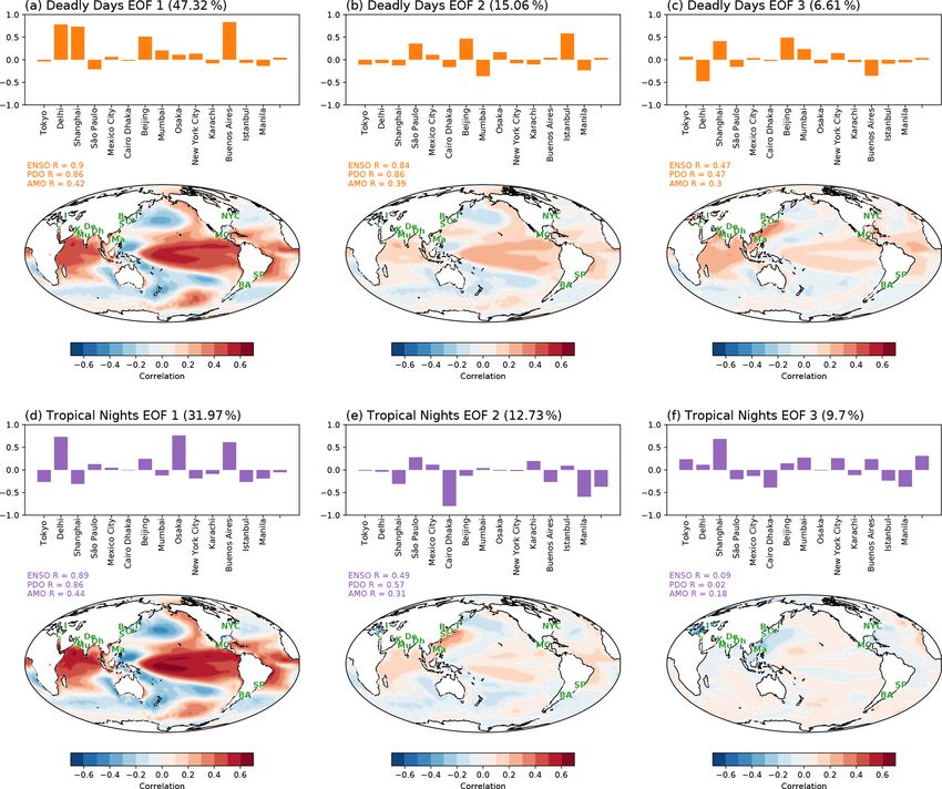
11890           J. Lee et al.: The effect of forced change and unforced variability on heat waves in a CO2 -warmed world

of population’s exposure to heat (Kharin et al., 2018), and the    2     Data
heat wave magnitude index (Russo et al., 2017). In this study,
we utilize four locally defined heat wave indices from Fischer     2.1    MPI–GE ensembles
and Schär (2010) and Perkins et al. (2012) in terms of the
duration, frequency, amplitude, and mean. We also focus on         Simulation data in this study come from an ensemble of runs
consecutive-day extremes, which are known to cause more            of the Max Plank Institute Earth System Model, collectively
harm than single-day events (Baldwin et al., 2019; Simolo          known as the MPI Grand Ensemble (MPI–GE) project (Ma-
et al., 2011; Tan et al., 2010). In addition, because the com-     her et al., 2019). Each of the 28 ensemble members branches
bined effect of temperature and humidity is known to affect        from different points of a 2000-year preindustrial control
human health by reducing the body’s ability to cool itself         run and is integrated for 150 years, forced by a CO2 con-
through perspiration, wet bulb temperature is frequently ana-      centration increasing at 1 % yr−1 (hereafter, 1 % runs). Be-
lyzed (Kang and Eltahir, 2018). Wet bulb temperature is also       cause the radiative forcing scales the log of the CO2 concen-
closely associated with moist thermodynamics that drive the        tration, the 1 % runs feature radiative forcing that increases
heat wave (Schwingshackl et al., 2021; Zhang et al., 2021),        approximately linearly in time. We analyze 6 h output, with
so we will analyze wet bulb temperature too.                       1.875◦ × 1.875◦ spatial resolution, which is the original res-
   Climate extremes are always a combination of long-term          olution of the model output for land areas between 60◦ N and
forced climate change acting in concert with unforced vari-        60◦ S. Our analysis will focus on 2 m temperature (hereafter,
ability (Deser et al., 2012). Thus, characterizing and quanti-     t2m) and 2 m dew point temperature (d2m), from which 2 m
fying both long-term change due to external forcing and the        relative humidity (RH) and wet bulb temperature (w2m) are
unforced variability in the climate system is crucial for as-      calculated, using the methods of Davies-Jones (2008) with a
sessing the future risk of extreme events. There have been         predesigned module named HumanIndexMod (Buzan et al.,
numerous studies that link dominant modes of unforced              2015).
variability to extreme events. For example, previous studies          Unforced variability in the climate system generates un-
have investigated temperature connections with the El Niño–        certainties in the projection of the climate by impacting the
Southern Oscillation (ENSO; Thirumalai et al., 2017; Meehl         dynamic component of the climate, especially for extreme
et al., 2007), the Pacific Decadal Oscillation (PDO; Birk et       events (Kay et al., 2015; Thompson et al., 2015). One way to
al., 2010), and the Atlantic Multidecadal Oscillation (AMO;        analyze the impact of unforced variability in a climate sys-
Zhang et al., 2020; Mann et al., 2021). The effect of climate      tem is to use an initial-condition ensemble. Each member of
extremes on different populations depends on numerous fac-         the initial-condition ensemble is generated by perturbating
tors, including the level of economic development, with im-        the initial conditions of single climate model. This pertur-
pacts of heat extremes being more severe in less econom-           bation will then propagate to generate different sequence of
ically developed countries (Diffenbaugh and Burke, 2019;           climate, such as ENSO, PDO, etc. (Deser et al., 2012; Kay
Harrington et al., 2016; King and Harrington, 2018; de Lima        et al., 2015). In this paper, we use the ensemble to allow us
et al., 2021). For example, as temperatures go up, an in-          to estimate the impact of unforced variability in temperature
creased energy demand to cool buildings will be required           extremes.
(Parkes et al., 2019; Sivak, 2009) in metropolitan areas. But         Since the model used only considers CO2 forcing without
this requires resources to both install air conditioning and op-   aerosols, and it represents a continuously warming climate,
erate it. The greater impacts of extreme heat in economically      one might question if the model simulation accurately rep-
less developed regions in a warmer climate have been dis-          resents the real climate. To judge the fidelity of the simu-
cussed in multiple studies (Marcotullio et al., 2021; Russo et     lations, we compare 15 years (2003–2017) of ERA-Interim
al., 2019).                                                        reanalysis data (Dee et al., 2011) from the European Centre
   In this paper, a single-model initial-condition ensemble of     for Medium-Range forecast (ECMWF) with 15 years of the
28 simulations of a global climate model (GCM) are used to         MPI–GE 1 % ensemble which have the same ensemble and
quantify heat and humidity extremes in a warmer world. We          global average temperatures (years 39–53); in the rest of the
use population data to look at the population risk for mor-        paper, we will refer to these as the reference periods. In both
tality events in the daytime (Mora et al., 2017) and night-        data sets, we then calculate 90th percentile and mean t2m and
time (Chen and Lu, 2014). We also utilize per capita gross         w2m for each grid point. This calculation was done for each
domestic product (GDP per capita) data to investigate how          member of the model ensemble. For each of the four values
climate change impacts extreme heat events on different lev-       (90th percentile – t2m and w2m; mean – t2m and w2m), we
els of economic status. To quantify the impact on energy de-       determine if the values from the reanalysis fall into the spread
mand, we also quantify the changes in cooling degree days          of the 28 ensemble members of the 1 % runs. For each grid
and warming degree days.                                           point, if the reanalysis value falls within the ensemble spread,
                                                                   we mask out the grid point; if not, we plot how far the reanal-
                                                                   ysis value is from the closest member of the 1 % ensemble
                                                                   (Fig. 1).

Atmos. Chem. Phys., 21, 11889–11904, 2021                                          https://doi.org/10.5194/acp-21-11889-2021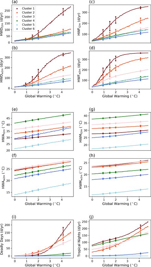
J. Lee et al.: The effect of forced change and unforced variability on heat waves in a CO2 -warmed world                       11891

Figure 1. Difference of 1 % CO2 runs compared with ERA-Interim in the same level of global warming (0.87 ◦ C). The grid points where
ERA-Interim falls within the ensemble spread of 1 % runs are masked with gray, while other grid points show the difference between the
nearest ensemble member and ERA-Interim for the (a) 90th percentile of the 15-year daily average t2m, (b) the mean of 15-year daily
average t2m, the (c) 90th percentile of 15-year daily average w2m, and (d) the mean of 15-year daily average w2m.

   Generally, the 1 % runs overpredict t2m and w2m in                boxes surrounding the MPI grid centers. In our population-
Northern Hemisphere (NH) and underpredict in Southern                weighted calculations, we assume that the relative distribu-
Hemisphere (SH), except for India. This difference is consis-        tion of population remains fixed into the future.
tent with the fact that the 1 % models do not contain aerosol           Gridded GDP per capita data (Kummu et al., 2019) be-
forcing, which should lead to biases of the sign seen in Fig. 1.     tween 1990 and 2015 are used to estimate the risk of heat
The w2m shows a larger area of differences than t2m, which           extreme events for different levels of wealth. These data are
suggests that there are larger biases in the dew point, which        regridded from the original 5 × 5 latitude–longitude spatial
is needed in the calculation (Davies-Jones, 2008). The area-         resolution to the MPI model’s resolution of 1.875◦ × 1.875◦
weighted averages of these differences are −0.08, −0.03,             by averaging the GDP inside the grid box. When doing this
−0.04, and −0.11 ◦ C globally for 90th percentile t2m, mean          average, per capita GDP was weighted by population and
t2m, 90th percentile w2m, and mean w2m, respectively,                also averaged over the 1990–2015 period. We assume that
which means that the model is, on average, underpredicting           the relative percentile of GDP per capita for each grid point
land temperature. Breaking down to the Northern and South-           is fixed into the future, so changes in climate risk are due
ern hemispheres, the bias is 0.20, 0.21, 0.15, and 0.14 ◦ C          to exposure to warmer climate extremes and not changes in
in the NH and −0.64, −0.54, −0.36, and −0.44 ◦ C in the SH,          relative per capita wealth.
confirming that the model is overpredicting land temperature
in the NH and underpredicting land temperature in the SH.
   To quantify the impact of the biases in Fig. 1 on the occur-      3     Method of analysis
rence of heat extremes, we will perform sensitivity tests on
                                                                     3.1    Global warming
the calculations by adding to each grid point of each member
of the ensemble the average differences between the ensem-           Global warming is defined as the global and annual average
ble average t2m and w2m and the reanalysis. By evaluating            temperature increase compared to the average of first 5 years
how much our results change, we come up with an estimate             of the 1 % run. We find that ensemble and global average t2m
of the impact of model biases on our results. As we will show        reaches 1.5, 2, 3 and 4 ◦ C in years 59, 76, 108, and 133, re-
later, these biases have little impact on the results of the pa-     spectively, and reaches 4.6 ◦ C at the end of the 150-year run.
per.                                                                 The increase in the global average temperature is nearly lin-
                                                                     ear for both t2m and w2m, consistent with a linear ramping
2.2   Global population and GDP per capita data                      of the forcing (Buzan and Huber, 2020).
                                                                        The focus of the paper will be on heat extremes at 1.5,
Global population data from the NASA Socioeconomic Data              2 and 3 ◦ C. The 1.5 and 2 ◦ C thresholds are the limits de-
and Applications Center (SEDAC, 2018) are used to weight             scribed in the Paris Agreement, while 3 ◦ C is the warming
the heat wave indices by population. The data represent the          we are presently on track for (Hausfather and Peters, 2020).
population in the year 2015 at 30×30 latitude–longitude spa-
tial resolution, and we regridded this to the 1.875◦ × 1.875◦
grid of the MPI model by summing the values in grid

https://doi.org/10.5194/acp-21-11889-2021                                           Atmos. Chem. Phys., 21, 11889–11904, 2021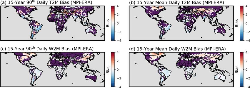
11892               J. Lee et al.: The effect of forced change and unforced variability on heat waves in a CO2 -warmed world

Table 1. Explanation of heat wave indices used in this study.

  Acronym            Index                 Definition                                                                                      Units
  HWDt2m/w2m         Heat wave duration    Length of longest period of consecutive heat wave days in a year                                No. of days
  HWFt2m/w2m         Heat wave frequency   Total number of heat wave days in a year                                                        No. of days
  HWAt2m/w2m         Heat wave amplitude   Maximum temperature over all heat wave days in a year                                           ◦C
  HWMt2m/w2m         Heat wave mean        Average temperature over all heat wave days in a year                                           ◦C
  Deadly days        Deadly days           Daily maximum wet-bulb temperature over 26 ◦ C                                                  No. of days
  Tropical nights    Tropical nights       Daily minimum temperature over 25 ◦ C                                                           No. of days
  CDDs               Cooling degree days   Sum of positive values after removing 18 ◦ C from daily average temperature                     Degree days
  HDDs               Heating degree days   Absolute value of sum of negative values after removing 18 ◦ C from daily average temperature   Degree days

3.2   Heat wave indices                                                        events per year, we increase this threshold to 26 ◦ C in our
                                                                               analysis. We could have chosen higher w2m values, but any
Identification of heat waves is done in several steps. First,                  choice in this range is associated with negative impacts, so
for each grid point, we smooth a daily maximum tempera-                        we have chosen a value near the bottom of the range where
ture (determined form 6 h temperatures) using a 15 d moving                    mortality occurs in order to maximize the signal in the model
window for the first 5 years of 1 % runs, which is the period                  runs.
before significant warming has occurred. Then, the 90th per-                      A warm nighttime minimum temperature can be as impor-
centile of the smoothed daily maximum temperature for the                      tant as a high maximum temperature for human health and
first 5 years was calculated at each grid point (Fischer and                   mortality (Argaud et al., 2007; Patz et al., 2005), so we de-
Schär, 2010). This value is used as a threshold for the heat                   fine “tropical nights” as a daily minimum t2m over 25 ◦ C
waves at that grid point. Then we calculate the heat wave                      (Lelieveld et al., 2012).
days, defined as days that exceed the threshold for 3 or more
consecutive days (Baldwin et al., 2019).                                       3.4    Cooling degree days and heating degree days
   We then define four indices to represent the characteristics
of these heat waves. To determine the occurrence of events,                    To assess the economic and energy impact of heat ex-
the heat wave duration (HWD; longest heat wave of the year)                    tremes, cooling degree days (CDDs) and heating degree
and heat wave frequency (HWF; total number of heat wave                        days (HDDs) are calculated. CDDs and HDDs are metrics
days in a year) are calculated. From an intensity perspec-                     of the energy demand to cool and heat buildings. For each
tive, the heat wave amplitude (HWA; maximum temperature                        grid point, the annual CDD is calculated by subtracting 18 ◦ C
during heat wave days during a year) and heat wave mean                        from the daily average temperature and summing only the
(HWM; mean temperature during heat wave days in a year)                        positive values over the year. The HDD is the absolute value
are selected. These indices are also calculated in an analo-                   of the sum of the negative values. Previous studies reported
gous fashion for the wet-bulb temperature (w2m), since the                     that CDDs and HDDs are closely related to energy consump-
wet bulb temperature is arguably more relevant for human                       tion (Sailor and Muñoz, 1997).
health (Heo et al., 2019; Morris et al., 2019; Buzan and Hu-
ber, 2020). These indices are summarized in Table 1.                           4     Results

3.3   Deadly days and tropical nights                                          4.1    Impact of unforced variability in climate on
                                                                                      regional heat extremes
Heat wave thresholds are different for each grid point be-
cause they are based on preindustrial temperatures at that                     To investigate the impact of unforced variability in more re-
grid point. Combined with regional differences in the ability                  gional heat extremes, we take the 15 largest cities by popula-
to adapt, this means that heat waves in different regions may                  tion (Fig. 2a) and determine the number of deadly days and
have different implications for human society. We, therefore,                  tropical nights over time by averaging the 3 × 3 grid points
also count the number of days in each year with daily maxi-                    surrounding the city and only including the land grid points.
mum w2m above 26 ◦ C, which we refer to as “deadly days”.                      Figure 2b–d depict the ensemble-averaged number of deadly
We note that other values could be chosen (Liang et al.,                       days and tropical nights, as well as the spread between the
2011), with higher values occurring less frequently but with                   ensemble members. The error bars in Fig. 2b–d show the
more significant impacts. This value is based on the analysis                  highest and lowest values of the extremes.
of Mora et al. (2017), who demonstrated that a w2m of about                       This difference within the ensemble is the result of un-
24 ◦ C is the threshold at which fatalities from heat-related                  forced variability. For all 15 cities, the average spread in the
illness occur. However, since we find that there are some re-                  number of deadly days at 1.5, 2.0, 3.0, and 4.0 ◦ C of global
gions that already experience over 9 months of 24 ◦ C w2m                      warming between the ensemble members with maximum and

Atmos. Chem. Phys., 21, 11889–11904, 2021                                                          https://doi.org/10.5194/acp-21-11889-2021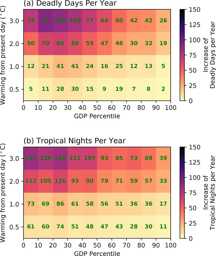
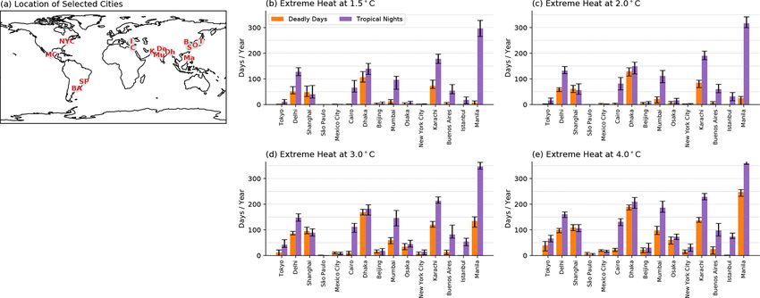
J. Lee et al.: The effect of forced change and unforced variability on heat waves in a CO2 -warmed world                                11893

Figure 2. (a) Location of 15 largest cities in the world and the number of annual heat extremes at (b) 1.5, (c) 2.0, (d) 3.0, and (e) 4.0 ◦ C of
global warming. Orange (purple) bars represent the ensemble average annual number of deadly days (tropical nights), averaged 5 years after
each level of warming is exceeded. The number of heat extreme days are calculated by averaging a 3 × 3 land-only grid covering the selected
city. Error bars represent the values of maximum and minimum ensemble members.

minimum numbers is 14.3, 15.1, 20.6, and 21.9 d yr−1 . For                lying physical mechanisms, an empirical orthogonal func-
tropical nights, the spread is 29.3, 27.7, 29.1, and 26.7 d yr−1 .        tion (EOF) analysis (North, 1984) was performed on the de-
So, on average, unforced variability can change the number                trended and normalized time series of deadly days and trop-
of extreme days and nights by a few weeks per year. There                 ical nights for the 15 cities. For each city, the 28 ensemble
is no significant variance of ensemble spread between the                 members are concatenated together (total of 28 × 150 years)
cities, except for cities with very low ensemble-averaged val-            in order for all ensembles to share the same EOF. In this way,
ues (e.g., Mexico City at 1.5 ◦ C warming) or very high values            we aim to find the dominant drivers of unforced variability
(e.g., tropical nights in Manila at 4.0 ◦ C warming). However,            that impacts heat extremes in the largest cities around the
for the cities that do not see a large increase in extreme tem-           world.
peratures (e.g., New York City), this represents a very large                The first three EOF patterns for each city are plotted in
fraction of the predicted change of extremes, while for cities            Fig. 3 as bars. The first EOF mode of deadly days shows
that experience a much larger increase (e.g., Manila), it rep-            large values for Delhi, Shanghai, Dhaka, and Karachi, while
resents a smaller percentage.                                             cities in other regions show lower values. The second and
   As discussed in Sect. 2.1, we examine the sensitivity of               third EOFs for deadly days show more variability between
our results to potential biases of the model by recalculating             the cities. The first EOF for tropical nights (Fig. 3d) shows
the deadly days and tropical nights using model data after                large positive values for cities in the India–Pakistan region,
adding in the bias estimated by a comparison to the reanaly-              with other cities showing smaller magnitude changes. The
sis. The average difference of deadly days in the sensitivity             second EOF shows large negative values in Cairo, Istanbul,
test (absolute difference) at 1.5, 2.0, 3.0, and 4.0 ◦ C warming          and Manila, while the third EOF for tropical nights shows
is 2.1, 2.5, 5,5, and 7.6 d yr−1 when averaged over 15 cities.            more variability between the cities.
The standard deviation of the difference calculated between                  The PC (principal component) time series are projected
the cities is 2.5, 3.4, 6.7, and 9.7 d at each level of warm-             onto detrended annual sea surface temperature (SST) anoma-
ing. For tropical nights, sensitivity test produced differences           lies. This allows us to investigate how heat extreme events in
of 3.6, 3.6, 5.3, and 3.5 d yr−1 at each level of warming, with           15 major cities are associated with global modes of unforced
standard deviations within the ensemble of 3.6, 4.9, 6.9, and             variability. Maps of correlation coefficients are also plotted in
1.8 d. Thus, model biases are unlikely to have a large impact             Fig. 3. Characteristic patterns for ENSO (Trenberth and Na-
on our results.                                                           tional Center for Atmospheric Research Staff, 2020), PDO
   Previous work has attempted to distinguish the origin and              (Deser et al., 2016), and AMO (Trenberth et al., 2020) are
mechanisms of unforced variability in temperature and tem-                calculated for each ensemble using all 150-years of SSTs,
perature extremes (Meehl et al., 2007; Zhang et al., 2020;                and the pattern is averaged over the ensembles to come up
Birk et al., 2010). To probe the statistical modes of variabil-           with a single ENSO, PDO, and AMO SST pattern for the en-
ity affecting this ensemble spread and to identify the under-             semble. Then, those patterns are compared with the PC pro-

https://doi.org/10.5194/acp-21-11889-2021                                                 Atmos. Chem. Phys., 21, 11889–11904, 2021
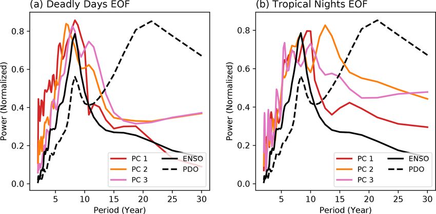
11894            J. Lee et al.: The effect of forced change and unforced variability on heat waves in a CO2 -warmed world

Figure 3. The first three EOFs of annual values of deadly days (a–c) and tropical nights (d–f) in the world’s 15 largest cities. For each panel,
the bar graph shows the EOF pattern of the number of heat extreme days per year. Contour plots shows the SST pattern associated with the
EOF mode, obtained by projecting each mode of PC onto SST anomalies. Ensemble members are averaged to yield the SST pattern. Pattern
correlations with major modes of climate variability (ENSO, PDO, and AMO) are also shown, as discussed in the text.

jection on SST to see how PC-projected SSTs resemble the                  rence of deadly days in these large cities is strongly regulated
patterns of unforced variability. Correlation coefficients be-            by ENSO. This may be a consequence of the fact that these
tween the standard climate indices and PC-projected SST is                large cities are mostly located near the ocean and at lower lat-
shown in the lower panel of Fig. 3 as numbers. All of the                 itudes. The third deadly day PC has lower correlations with
projections of deadly day PCs and projections of the first two            the ENSO or PDO indexes, so it is harder to draw firm con-
modes of tropical nights show patterns similar to ENSO and                clusions about the mechanism behind it. Also, higher modes
PDO.                                                                      of EOFs are unlikely to refer to a single mode of climate
   Power spectra of the PCs are calculated individually for               due to the orthogonality constraints between each mode. The
each ensemble member, and then the ensemble average is                    tropical night PCs also show peaks at ENSO periods (Fig. 4b)
plotted Fig. 4. Overall, the spectra of the deadly day PCs                suggesting that, like deadly days, tropical night variability is
look very much like the spectrum for ENSO, and it notably                 controlled by ENSO.
does not have the ∼ 20-year peak of the PDO spectrum. This
tells us that, in this model at least, the variability in the occur-

Atmos. Chem. Phys., 21, 11889–11904, 2021                                                   https://doi.org/10.5194/acp-21-11889-2021
J. Lee et al.: The effect of forced change and unforced variability on heat waves in a CO2 -warmed world 11895
Figure 4. Frequency power spectrum of ENSO, PDO, and PC of the first three EOF modes for (a) deadly days and (b) tropical nights. ENSO
is calculated with the Niño 3.4 index, and PDO is calculated as a leading EOF of SST anomaly in the North Pacific basin. Monthly SST data
are used for both ENSO and PDO, and then each index is averaged over the year to have consistency with deadly days and tropical nights.
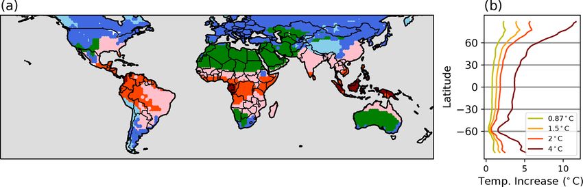
Figure 5. (a) Clustered regions via K-means clustering. Characteristics of each cluster are listed in Table 2. (b) Zonal average of temperature
increases at the time of 0.87 (our reference period), 1.5, 2, and 4 ◦ C of global warming compared to the preindustrial baseline in the 1 %
runs. Temperatures are averaged over a 5-year period after each warming threshold is exceed in the model.
4.2 Cluster analysis and population risk of heat wave Figure 5a shows the cluster value that most ensembles as-
indices signed to each grid point, and it shows distinct geographi-
cal characteristics, as summarized in Table 2 (the result of
We calculate HWD, HWF, HWA, and HWM for both t2m clustering shows little difference between individual ensem-
and w2m each year at each grid point, which generates eight ble members). As might be expected from how we calculated
different 150-year time series for each of the 28 ensemble the 16 variables for clustering, each cluster shows a different
members. Each time series at each grid point is regressed evolution of heat extremes in a warmer world (Fig. 6). Al-
vs. time, yielding a slope and the intercept for each time se- though the warming signal is the largest in the polar regions
ries in all 28 ensemble members. The 16 variables (8 heat (Fig. 5b), the largest increases in HWD and HWF are found
wave indices × 2 slope and intercept) are then utilized as a at lower latitudes (in cluster 1 and 2 in Fig. 6a–d). This is
predictor variable for K-means clustering (Likas et al., 2003) mostly due to low variability in these regions compared to
to categorize the spatial variation in heat waves using the Eu- polar regions, making it easier for a trend to exceed the heat
clidean distance of its predictor variables (16 variables). With wave threshold.
slope and intercept, we can characterize the heat indices of These results are insensitive to potential model biases.
each grid point with response to CO2 forcing (slope) and cli- Sensitivity tests show that adding the bias to the model
matology (intercept). The number of clusters in this study changes HWD, HWF, deadly days, and tropical nights by less
is set to 6, using the elbow method (Syakur et al., 2018). than 5 % for all metrics and clusters. For HWA and HWM,
When using five clusters, we find that two clusters (the light the difference caused by adding the bias was less than 1 ◦ C
and dark blue regions in Fig. 5a) merge, and when using for all metrics and clusters, suggesting that the impact of
seven clusters, we find that one cluster (the dark blue region model biases is small in this analysis.
in Fig. 5a) divides into two separate clusters.
https://doi.org/10.5194/acp-21-11889-2021 Atmos. Chem. Phys., 21, 11889–11904, 2021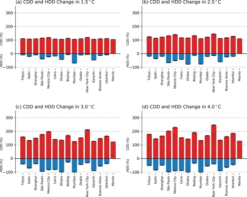
11896           J. Lee et al.: The effect of forced change and unforced variability on heat waves in a CO2 -warmed world

Figure 6. Evolution of each index averaged over each cluster. Colors are consistent with Fig. 5 and Table 2. The values of each metric are
calculated by averaging the grid points that belong to each cluster. This was done for each ensemble member, and then the ensemble average
is plotted. Vertical lines with dots show the maximum and minimum of 28 ensemble members at each threshold of warming to represent the
spread between the ensemble members.

Atmos. Chem. Phys., 21, 11889–11904, 2021                                                https://doi.org/10.5194/acp-21-11889-2021
J. Lee et al.: The effect of forced change and unforced variability on heat waves in a CO2 -warmed world                              11897

Table 2. Percentage area and major regions belonging to each cluster. Clusters are identified only for the global land areas.

 Cluster   Color            Area     Major regions                                                        Cluster name
                       percentage
                              (%)
 1         Maroon            2.95    Indonesia, Malaysia, Cameroon, and Gabon                             Tropical West Pacific
 2         Orange           12.34    Northern South America and central Africa                            Tropical Africa and North America
 3         Pink             22.70    India, Southeast Asia, eastern South America, and southeastern USA   Subtropical Asia and America
 4         Green            21.55    Northern Africa, the Middle East, and Australia                      Deserts
 5         Sky blue          7.69    Himalayas and Andes                                                  Mountain ranges
 6         Blue             32.75    Canada, northwestern US, and Russia                                  Subpolar regions

   For HWA and HWM, the rate of increase is similar for                   2.5 ◦ C. Given that the planet has already warmed about 1 ◦ C
all clusters, with increases in HWAt2m and HWAw2m of                      above preindustrial levels, this suggests that the world should
1.45 ◦ C per degree of global average warming, respectively,              presently be experiencing a rapid increase in wet bulb ex-
and HWMt2m 0.85 ◦ C per degree of global average warming,                 treme frequency, particularly in the tropics. This is related to
respectively, and HWMt2m and HWMw2m of 0.66 ◦ C per de-                   the increased slope in Fig. 6, in which values of HWDw2m
gree of global average warming and 0.47 ◦ C per degree of                 and HWFw2m for clusters 1 and 2 increase rapidly until
global average warming, respectively (Fig. 6e–h). The excep-              3.0 and 2.0 ◦ C of global warming. At warmer temperatures,
tion is HWAt2m in cluster 6. The large increase in HWAt2m in              HWDw2m and HWFw2m reach a plateau, since values over
this region is connected to the strong global warming signal              300 d yr−1 mean there is little room for additional increases.
in high latitudes that has been predicted for decades and is              For HWAt2m/w2m and HWMt2m/w2m , the increase is mostly
now observed (Stouffer and Manabe, 2017).                                 linear. Also note that, at 3 ◦ C of global warming, the 90th per-
   Turning to deadly days (Fig. 6i), we find that a substan-              centile of population-weighted HWAw2m reaches over 29 ◦ C,
tial increase occurs in cluster 1 after 2.0 ◦ C of warming; this          which, while not immediately fatal to humans, may, never-
is important because it gives additional support for the Paris            theless, indicate great difficulty for even a developed society
Agreement’s aspirational goal of limiting global warming to               to adapt to.
2.0 ◦ C. Almost all increases in deadly days are in low lati-                Currently, 10 % of the total population faces more than
tudes (clusters 1, 2, and 3). For tropical nights, low latitudes          45 deadly days and 181 tropical nights per year. This grows
and deserts (cluster 4) contribute most of the increase. Fig-             to 65 and 195 d, respectively, at 1.5 ◦ C warming. With 2 ◦ C
ure 6 also shows the spread within the ensemble for each                  of global warming, 10 % of the population will face about
metric and cluster. We find that the spread for a cluster is              3 months of deadly days and 7 months of tropical nights ev-
generally small compared to the change over time and the                  ery year, and this increases to 4 and 8 months with 3 ◦ C of
difference between the clusters.                                          warming. Also, with 3 ◦ C of global warming, 5 % of the pop-
   We also generated indices weighted by global popula-                   ulation will be in an environment where 8 and 10 months a
tion. Heat wave indices for the 95th percentile of population             year are deadly days and tropical nights. Our sensitivity tests
(meaning 5 % of the population is exposed to higher values),              suggest that model bias generates less than 5 % differences
the 90th percentile of population, and the median of the pop-             for HWD, HWF, deadly days, and tropical nights for all met-
ulation are depicted in Fig. 7. Figure 7a shows that, with 3 ◦ C          rics and the percentile of population at every level of global
of warming, 5 % of the Earth’s population will experience                 warming, except when the metrics are near zero. Potential
heat waves lasting 122 d (standard deviation between ensem-               model biases also generate small differences in HWA and
ble members of 1σ = 17 d), 10 % of the population will ex-                HWM, with less than 1 ◦ C difference in all metrics for every
perience heat waves lasting 94 d (1σ = 7 d), and half of the              period. Furthermore, with 3 ◦ C of global warming, the min-
population will experience heat waves lasting around 50 d                 imum ensemble member of deadly days is above the maxi-
(1σ = 4 d). These are large increases over present-day values             mum ensemble of the present-day reference (0.87 ◦ C) for all
of 50, 42, and 21 d. The average of the standard deviation be-            population percentiles (5 %, 10 %, and 50 %). This occurs at
tween the ensemble members (calculated every year and then                2 ◦ C for tropical nights. Details of the ensemble spread are
averaged) is 10.6, 6.2, and 3.7 d for the 95th, 90th percentile,          also shown in Table 3.
and median, respectively. This is significantly smaller than                 It is notable that, although there is a large spread between
the values from the analyses of the cities in Fig. 2, where               the ensemble members in each city (Fig. 2), the spread in the
the unforced variability makes larger differences in the oc-              clusters (Fig. 6) and population-weighted metrics (Fig. 7) is
currence of heat waves.                                                   not as large. This emphasizes that the effect of unforced vari-
   The rate of increase in HWFw2m in Fig. 7d shows a rapid                ability might be large at small scales, but as the region ex-
increase until the global average warming reaches about                   pands, the impact of unforced variability decreases. This is

https://doi.org/10.5194/acp-21-11889-2021                                                Atmos. Chem. Phys., 21, 11889–11904, 2021
11898 J. Lee et al.: The effect of forced change and unforced variability on heat waves in a CO2 -warmed world Figure 7. Changes in population-weighted heat wave indices as a function of global average warming. Each line denotes one ensemble member for different percentiles of the population. Atmos. Chem. Phys., 21, 11889–11904, 2021 https://doi.org/10.5194/acp-21-11889-2021
J. Lee et al.: The effect of forced change and unforced variability on heat waves in a CO2 -warmed world 11899
Table 3. Number of deadly days each percentile (p.) of the global population faces, with reference period (0.87 ◦ C) and 1.5, 2, 3, and 4 ◦ C
of global warming from the preindustrial condition. Standard deviations between the ensembles (1σ ) are also shown.
Global warming
Population 0.87 ◦ C 1.5 ◦ C 2.0 ◦ C 3.0 ◦ C 4.0 ◦ C
Deadly 95th p. 85 (±7) 105 (±10) 125 (±7) 161 (±12) 229 (±15)
days 90th p. 45 (±5) 65 (±10) 86 (±8) 132 (±12) 198 (±12)
50th p. 0.3 (±0.1) 1.5 (±1.3) 5 (±2) 23 (±4) 63 (±5)
Tropical 95th p. 211 (±11) 232 (±14) 253 (±13) 306 (±17) 358 (±3)
nights 90th p. 280 (±7) 195 (±9) 205 (±9) 232 (±12) 277 (±14)
50th p. 15 (±4) 27 (±7) 41 (±6) 71 (±6) 102 (±4)
also found in Table 3, where, in each case, the standard de-
viation between ensembles is less than 20 % of the average,
except in a few cases. This indicates that unforced variability
will generally play a minor role in determining global ex-
posure to temperature above thresholds, although different
people may be affected in different realizations of unforced
variability.
In addition, with 1.5 ◦ C of global warming, the lowest en-
semble of the 90th percentile of HWDt2m , HWDw2m , and
HWFt2m exceeds the highest ensemble of the same metric in
the current climate (red lines in Fig. 7). With 2 ◦ C of warm-
ing, the minimum ensemble of HWDt2m/w2m , HWFt2m/w2m ,
HWMw2m , and tropical nights exceed the maximum ensem-
ble of the current climate, and with 2.5 ◦ C of warming, the
minimum ensemble of all metrics exceeds the maximum en-
semble of the same metric in the current climate. Thus, this
model predicts that the occurrence of extremes will soon be
able to exceed values likely possible in our present climate
for these metrics.
4.3 Analysis on GDP per capita
It is well known that not everyone is equally vulnerable to
extreme weather, with rich, relatively more developed com-
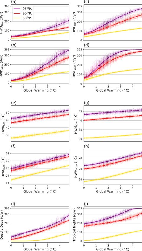
munities having more resources to deal with extreme events Figure 8. Increase in (a) deadly days and (b) tropical nights com-
than poorer communities. In that context, the global gridded pared to the reference period (0.87 ◦ C of warming), binned by the
GDP per capita is used to calculate average risk at each level percentile of GDP per capita at selected levels of warming com-
of wealth. The ensemble-averaged result is depicted in Fig. 8, pared to reference climate (calculated by subtracting reference val-
which shows the absolute number of deadly days and tropical ues, shown as a heat map), averaged over the population within
nights, as well as the increase in the number of deadly days the GDP percentile (for example, averaged over population in 0–
and tropical nights that each economic level experiences rel- 10 percentile of GDP) and over all ensemble members for 5-year
ative to the reference period warming of 0.87 ◦ C. This plot window after each level of warming first occurs. Green text inside
assumes that the relative distribution of population and GDP the heat map represents the absolute number of deadly days and
tropical nights in each level of warming.
remains fixed through time. Our sensitivity tests show that
the model bias yields small differences in the results, with
less than 5 % difference in both the absolute number of ex-
treme events and the changes in extremes. centile of GDP, and for tropical nights, the increase is largest
For each level of warming, we find that the lower GDP below the 30th percentile of GDP. The regions that con-
regions will experience not only higher absolute numbers of tribute the most for the low GDP percentiles are in Southeast
extreme temperature days but also the largest increases. For Asia, including Myanmar, Laos, and Cambodia, and tropi-
deadly days, the increase is largest between 10th to 40th per- cal Africa, including the Democratic Republic of the Congo,
https://doi.org/10.5194/acp-21-11889-2021 Atmos. Chem. Phys., 21, 11889–11904, 202111900 J. Lee et al.: The effect of forced change and unforced variability on heat waves in a CO2 -warmed world
Figure 9. Change (in percentage) of ensemble-averaged cooling degree days (CDD; red) and heating degree days (HDD; blue) compared
to the reference climate (0.87 ◦ C) in the 1 % CO2 experiments at the time they reach the global mean temperature thresholds of (a) 1.5 ◦ C,
(b) 2.0 ◦ C, (c) 3.0 ◦ C, and (d) 4.0 ◦ C, respectively. Error bars represent the standard deviation in CDD and HDD values between the ensemble
members.
Kenya, Uganda, Ethiopia, and the Republic of Sudan, which In contrast, average energy demand on cold days (HDDs)
are in clusters 1 and 2 in our cluster analysis (Fig. 5). The decreases by 21 %, 36 %, 59 %, and 65 % in cities consid-
maximum difference in heat wave days between the ensem- ered, compared to present day, partially offsetting the in-
bles is less than 25 % for all GDP and global warming levels. crease in energy required for cooling. Manila shows 0 %
change in HDDs for all periods, since Manila does not ex-
4.4 Energy demand on large cities perience HDD days in present or future periods. Sensitivity
tests also show less than a 1 % difference in HDD change due
Annual CDDs and HDDs have been calculated for the to model biases.
15 cities in Sect. 4.1. Both CDDs and HDDs are calculated
by averaging the CDD and HDD values of 3 × 3 grid points
surrounding each city, including only land grid points. CDD
5 Conclusion
and HDD values are then averaged for 5 years after global
warming reaches each levels of threshold. Figure 9 shows
In this study, we found that extreme heat events will be-
the percent change in CDDs and HDDs at 1.5, 2.0, 3.0, and
come more frequent and severe in a warming world. We find
4.0 ◦ C relative to the reference period CDD and HDD val-
that both forced and unforced variability play a key role in
ues. This was done for each city and for each ensemble
extreme heat events, highlighting the necessity of consid-
member. At 1.5, 2.0, 3.0, and 4.0 ◦ C warming, CDDs in the
ering both contributions to extreme heat. We also look at
15 cities increase by an average of 9 %, 22 %, 54 %, and
population-weighted and GDP-sorted statistics of extreme
70 %. Our sensitivity tests show that the application of the
heat in warmer world.
average model bias yields changes of less than 1 % in these
Our results show that ENSO is the dominant mode of un-
numbers. This suggests an enormous increase in energy re-
forced variability impacting the occurrence of extreme heat
quired for cooling.
and humidity events and that events tend to be synchronous
Atmos. Chem. Phys., 21, 11889–11904, 2021 https://doi.org/10.5194/acp-21-11889-2021J. Lee et al.: The effect of forced change and unforced variability on heat waves in a CO2 -warmed world 11901
in the world’s largest 15 cities. But while the impact of un- for a more detailed analysis (Dibike and Coulibaly, 2006;
forced variability might be significant regionally and tem- Wood et al., 2004). Also, land models with the capacity to de-
porarily, it becomes less important when one looks at larger compose the urban and rural environment could be applied in
aggregate regions. the same context (Bonan et al., 2002; Dickinson et al., 2006).
Looking at global population-weighted statistics, we Also, this study could gain further insights by considering
found that, with 1.5 ◦ C of global average warming, over changing population and socioeconomic distribution in the
10 % of the population will face heat waves of 45 ◦ C tem- future. Overall, however, none of these things are expected to
perature and 28 ◦ C wet-bulb temperatures. Furthermore, 5 % change the broad conclusion of this study that global warm-
of the population will face more than 105 d of deadly days ing will lead to increased exposure to extremes in heat and
and 232 d of tropical nights per year. With 3 ◦ C of warming, humidity.
which we are currently on track for, 10 % of the population
will experience over 132 d of deadly days and over 232 d of
tropical nights per year. Moreover, 10 % of the population Data availability. The 6 h 1 % runs from MPI–GE can be dis-
will face a 47 ◦ C temperature and 30 ◦ C wet-bulb tempera- tributed upon request. ERA-Interim data are available from
ture. Given that these two metrics have important implica- the ECMWF archive (https://www.ecmwf.int/en/forecasts/datasets/
tions for human mortality, such increases may have signifi- reanalysis-datasets/era-interim, last access: October 2018) (Berris-
ford et al., 2018). Global population data are available from
cant impacts on human health globally.
the NASA SEDAC archive (https://doi.org/10.7927/H49C6VHW)
Sorting heat and humidity events by wealth, we confirm (CIESIN, 2020). Global GDP per capita can be obtained from
that the increasing frequency and severity of extreme events Kummu et al. (2019) (https://doi.org/10.5061/dryad.dk1j0).
will fall mostly on poorer people. To further investigate some
economic impacts of increasing heat extremes, cooling de-
gree days (CDDs) and heating degree days (HDDs) are cal- Author contributions. JL, JM, and AD conceptualized the project.
culated for the world’s 15 largest cities. Energy demand for The data curation was done by JL and AD, while JL and JM con-
cooling (CDDs) increases by an average of 9 % for 1.5 ◦ C ducted the formal analysis. AD acquired the funding, while JL and
and 54 % for 3.0 ◦ C of warming, while energy demand for JM led the investigation. JL took responsibility for the methodol-
heating (HDDs) decreases by 21 % and 59 %. Since CDDs ogy, software, and visualization. AD administered and supervised
are known to have a piecewise linear relationship with the the project and acquired the resources. JL and AD wrote the paper.
energy consumption, with the slope increasing with higher
CDDs (De Rosa et al., 2014; Shin and Do, 2016), increas-
ing CDDs in a warmer world could be one of the factors Competing interests. The authors declare that they have no conflict
driving increased economic inequity from global-warming- of interest.
related heat extremes, due to relatively high costs and the
need for energy in the poorest countries.
Disclaimer. Publisher’s note: Copernicus Publications remains
Uncertainties in this analysis include our use of gridded
neutral with regard to jurisdictional claims in published maps and
6 h climate model output. More detailed analysis could be institutional affiliations.
done with climate simulations with higher temporal and spa-
tial resolution. The model has biases relative to measure-
ments, potentially due to the fact that there are no aerosols Financial support. This research has been supported by the Di-
in the forcing, which is another source of uncertainty. This vision of Atmospheric and Geospace Sciences (grant nos. AGS-
was tested by adding the difference between the ensemble 1661861 and AGS-1841308) to Texas A & M University.
average and the reanalysis data to the model fields and re-
computing the heat wave indices. In general, the impact of
this bias was not important. In future analyses, this could be Review statement. This paper was edited by Mathias Palm and re-
better resolved with use of multimodel ensembles or detailed viewed by Sabine Undorf and one anonymous referee.
bias correction of the model.
Another uncertainty is that our runs are continuously
warming, and it is possible that an equilibrium world at any
given temperature may experience a different occurrence of
extremes than in the runs in this paper. Additionally, since an
increasing proportion of the population is expected to live in
dense metropolitan areas, there is also the possibility that ac-
tual heat and humidity extremes that populations experience
could be more severe than the gridded data due to local phe-
nomena such as the urban heat island effect (Murata et al.,
2012). Statistical or dynamical downscaling could be used
https://doi.org/10.5194/acp-21-11889-2021 Atmos. Chem. Phys., 21, 11889–11904, 202111902 J. Lee et al.: The effect of forced change and unforced variability on heat waves in a CO2 -warmed world
References A. P., Monge-Sanz, B. M., Morcrette, J. J., Park, B. K., Peubey,
C., de Rosnay, P., Tavolato, C., Thepaut, J. N., and Vitart, F.: The
Arbuthnott, K., Hajat, S., Heaviside, C., and Vardoulakis, S.: ERA-Interim reanalysis: configuration and performance of the
Changes in population susceptibility to heat and cold over time: data assimilation system, Q. J. Roy. Meteorol. Soc., 137, 553–
assessing adaptation to climate change, Environ. Health, 15, 73– 597, https://doi.org/10.1002/qj.828, 2011.
93, 2016. de Lima, C. Z., Buzan, J. R., Moore, F. C., Baldos, U. L. C., Huber,
Argaud, L., Ferry, T., Le, Q. H., Marfisi, A., Ciorba, D., M., and Hertel, T. W.: Heat stress on agricultural workers exac-
Achache, P., Ducluzeau, R., and Robert, D.: Short- and erbates crop impacts of climate change, Environ. Res. Lett., 16,
long-term outcomes of heatstroke following the 2003 heat 044020, https://doi.org/10.1088/1748-9326/abeb9f, 2021.
wave in Lyon, France, Arch. Intern. Med., 167, 2177–2183, De Rosa, M., Bianco, V., Scarpa, F., and Tagliafico, L. A.: Heat-
https://doi.org/10.1001/archinte.167.20.ioi70147, 2007. ing and cooling building energy demand evaluation; a simplified
Baldwin, J. W., Dessy, J. B., Vecchi, G. A., and Oppenheimer, model and a modified degree days approach, Appl. Energy, 128,
M.: Temporally Compound Heat Wave Events and Global 217–229, 2014.
Warming: An Emerging Hazard, Earths Future, 7, 411–427, Deser, C., Phillips, A., Bourdette, V., and Teng, H. Y.: Uncer-
https://doi.org/10.1029/2018ef000989, 2019. tainty in climate change projections: the role of internal variabil-
Berrisford, P., Dee, D., Poli, P., Brugge, R., Fielding, K., Fuentes, ity, Clim. Dynam., 38, 527–546, https://doi.org/10.1007/s00382-
M., and Simmons, A.: The ERA-Interim archive Version 2.0, 010-0977-x, 2012.
Shinfield Park, Reading, available at: https://www.ecmwf.int/ Deser, C., Trenberth, K., and National Center for Atmo-
en/forecasts/datasets/reanalysis-datasets/era-interim, last access: spheric Research Staff (Eds.): The Climate Data Guide:
October 2018. Pacific Decadal Oscillation (PDO): Definition and Indices,
Birk, K., Lupo, A. R., Guinan, P., and Barbieri, C.: The interan- available at: https://climatedataguide.ucar.edu/climate-data/
nual variability of midwestern temperatures and precipitation as pacific-decadal-oscillation-pdo-definition-and-indices (last
related to the ENSO and PDO, Atmosfera, 23, 95–128, 2010. access: March 2020), 2016.
Bonan, G. B., Oleson, K. W., Vertenstein, M., Levis, S., Zeng, X., Dibike, Y. B. and Coulibaly, P.: Temporal neural networks for down-
Dai, Y., Dickinson, R. E., and Yang, Z.-L.: The land surface cli- scaling climate variability and extremes, Neural Networks, 19,
matology of the Community Land Model coupled to the NCAR 135–144, https://doi.org/10.1016/j.neunet.2006.01.003, 2006.
Community Climate Model, J. Climate, 15, 3123–3149, 2002. Dickinson, R. E., Oleson, K. W., Bonan, G., Hoffman, F., Thornton,
Buzan, J. R. and Huber, M.: Moist heat stress on a hot- P., Vertenstein, M., Yang, Z.-L., and Zeng, X.: The Community
ter Earth, Annu. Rev. Earth Planet. Sci., 48, 623–655, Land Model and its climate statistics as a component of the Com-
https://doi.org/10.1146/annurev-earth-053018-060100, 2020. munity Climate System Model, J. Climate, 19, 2302–2324, 2006.
Buzan, J. R., Oleson, K., and Huber, M.: Implementation and com- Diffenbaugh, N. S. and Burke, M.: Global warming has increased
parison of a suite of heat stress metrics within the Commu- global economic inequality, P. Natl. Acad. Sci. USA, 116, 9808–
nity Land Model version 4.5, Geosci. Model Dev., 8, 151–170, 9813, 2019.
https://doi.org/10.5194/gmd-8-151-2015, 2015. Fischer, E. M. and Schär, C.: Consistent geographical patterns of
Chen, R. D. and Lu, R. Y.: Dry Tropical Nights and Wet Extreme changes in high-impact European heatwaves, Nat. Geosci., 3,
Heat in Beijing: Atypical Configurations between High Tem- 398–403, 2010.
perature and Humidity, Mon. Weather Rev., 142, 1792–1802, Harrington, L. J., Frame, D. J., Fischer, E. M., Hawkins, E.,
https://doi.org/10.1175/Mwr-D-13-00289.1, 2014. Joshi, M., and Jones, C. D.: Poorest countries experience ear-
Chow, W. T., Chuang, W.-C., and Gober, P.: Vulnerability to ex- lier anthropogenic emergence of daily temperature extremes,
treme heat in metropolitan Phoenix: spatial, temporal, and de- Environ. Res. Lett., 11, 055007, https://doi.org/10.1088/1748-
mographic dimensions, Profess. Geogr., 64, 286–302, 2012. 9326/11/5/055007, 2016.
CIESIN – Center for International Earth Science Information Net- Harrington, L. J., Frame, D., King, A. D., and Otto, F. E.: How un-
work: Columbia University Gridded Population of the World, even are changes to impact-relevant climate hazards in a 1.5 ◦ C
Version 4 (GPWv4): Population Density, Revision 11, NASA So- world and beyond?, Geophys. Res. Lett., 45, 6672–6680, 2018.
cioeconomic Data and Applications Center (SEDAC), [data set], Hausfather, Z., and Peters, G. P.: Emissions–the ‘business as
https://doi.org/10.7927/H49C6VHW, 2020. usual’story is misleading. Nature Publishing Group, 2020.
Dahl, K., Licker, R., Abatzoglou, J. T., and Declet-Barreto, J.: In- Heo, S., Bell, M. L., and Lee, J. T.: Comparison of health risks
creased frequency of and population exposure to extreme heat by heat wave definition: Applicability of wet-bulb globe tem-
index days in the United States during the 21st century, En- perature for heat wave criteria, Environ. Res., 168, 158–170,
viron. Res. Commun., 1, 075002, https://doi.org/10.1088/2515- https://doi.org/10.1016/j.envres.2018.09.032, 2019.
7620/ab27cf, 2019. Hoegh-Guldberg, O., Jacob, D., Bindi, M., Brown, S., Camilloni, I.,
Davies-Jones, R.: An efficient and accurate method for computing Diedhiou, A., Djalante, R., Ebi, K., Engelbrecht, F., and Guiot,
the wet-bulb temperature along pseudoadiabats, Mon. Weather J.: Impacts of 1.5 ◦ C global warming on natural and human sys-
Rev., 136, 2764–2785, 2008. tems, Global warming of 1.5 ◦ C, An IPCC Special Report, IPCC,
Dee, D. P., Uppala, S. M., Simmons, A. J., Berrisford, P., Poli, Switzerland, 2018.
P., Kobayashi, S., Andrae, U., Balmaseda, M. A., Balsamo, G., Kang, S. and Eltahir, E. A. B.: North China Plain threatened by
Bauer, P., Bechtold, P., Beljaars, A. C. M., van de Berg, L., Bid- deadly heatwaves due to climate change and irrigation, Nat.
lot, J., Bormann, N., Delsol, C., Dragani, R., Fuentes, M., Geer, Commun., 9, 2894, https://doi.org/10.1038/s41467-018-05252-
A. J., Haimberger, L., Healy, S. B., Hersbach, H., Holm, E. V., y, 2018.
Isaksen, L., Kallberg, P., Kohler, M., Matricardi, M., McNally,
Atmos. Chem. Phys., 21, 11889–11904, 2021 https://doi.org/10.5194/acp-21-11889-2021J. Lee et al.: The effect of forced change and unforced variability on heat waves in a CO2 -warmed world 11903 Kay, J. E., Deser, C., Phillips, A., Mai, A., Hannay, C., Strand, cock, R.: Global warming of 1.5 ◦ C, in: An IPCC Special Report G., Arblaster, J. M., Bates, S. C., Danabasoglu, G., Edwards, on the impacts of global warming of 1.5 ◦ C above pre-industrial J., Holland, M., Kushner, P., Lamarque, J. F., Lawrence, D., levels and related global greenhouse gas emission pathways, in Lindsay, K., Middleton, A., Munoz, E., Neale, R., Oleson, K., the context of strengthening the global response to the threat of Polvani, L., and Vertenstein, M.: The Community Earth Sys- climate change, sustainable development, and efforts to eradicate tem Model (CESM) Large Ensemble Project A Community Re- poverty, World Meteorological Organization, Geneva, 2018. source for Studying Climate Change in the Presence of Inter- Meehl, G. A., Tebaldi, C., Teng, H., and Peterson, T. C.: Current and nal Climate Variability, B. Am. Meteorol. Soc., 96, 1333–1349, future US weather extremes and El Niño, Geophys. Res. Lett., https://doi.org/10.1175/Bams-D-13-00255.1, 2015. 34, L20704, https://doi.org/10.1029/2007GL031027, 2007. Kharin, V. V., Flato, G. M., Zhang, X., Gillett, N. P., Melillo, J. M., Richmond, T., and Yohe, G. W.: Climate Change Im- Zwiers, F., and Anderson, K. J.: Risks from Climate Ex- pacts in the United States: The Third National Climate Assess- tremes Change Differently from 1.5 degrees C to 2.0 de- ment, US Global Change Research Program, Washington, DC, grees C Depending on Rarity, Earths Future, 6, 704–715, https://doi.org/10.7930/J0Z31WJ2, 2014. https://doi.org/10.1002/2018ef000813, 2018. Mora, C., Dousset, B., Caldwell, I. R., Powell, F. E., Geronimo, R. King, A. D. and Harrington, L. J.: The inequality of climate change C., Bielecki, C. R., Counsell, C. W., Dietrich, B. S., Johnston, from 1.5 to 2 ◦ C of global warming, Geophys. Res. Lett., 45, E. T., Louis, L. V., Lucas, M. P., McKenzie, M. M., Shea, A. 5030–5033, 2018. G., Tseng, H., Giambelluca, T., Leon, L. R., Hawkins, E., and Kummu, M., Taka, M., and Guillaume, J. H. A.: Data from: Trauernicht, C.: Global risk of deadly heat, Nat. Clim. Change, Gridded global datasets for Gross Domestic Product and Hu- 7, 501–506, https://doi.org/10.1038/Nclimate3322, 2017. man Development Index over 1990–2015 Dryad, [dataset], Morris, C. E., Gonzales, R. G., Hodgson, M. J., and Tustin, https://doi.org/10.5061/dryad.dk1j0, 2019. A. W.: Actual and simulated weather data to evaluate wet Lelieveld, J., Hadjinicolaou, P., Kostopoulou, E., Chenoweth, J., bulb globe temperature and heat index as alerts for occupa- El Maayar, M., Giannakopoulos, C., Hannides, C., Lange, M. tional heat-related illness, J. Occupat. Environ. Hyg., 16, 54–65, A., Tanarhte, M., Tyrlis, E., and Xoplaki, E.: Climate change https://doi.org/10.1080/15459624.2018.1532574, 2019. and impacts in the Eastern Mediterranean and the Middle East, Murata, A., Nakano, M., Kanada, S., Kurihara, K., and Sasaki, Climatic Change, 114, 667–687, https://doi.org/10.1007/s10584- H.: Summertime temperature extremes over Japan in the late 012-0418-4, 2012. 21st century projected by a high-resolution regional climate Liang, C., Zheng, G., Zhu, N., Tian, Z., Lu, S., and Chen, Y.: A new model, J. Meteorol. Soc. Jpn. Ser. II, 90, 101–122, 2012. environmental heat stress index for indoor hot and humid envi- North, G. R.: Empirical orthogonal functions and normal modes, J. ronments based on Cox regression, Build. Environ., 46, 2472– Atmos. Sci., 41, 879–887, 1984. 2479, 2011. Parkes, B., Cronin, J., Dessens, O., and Sultan, B.: Climate change Likas, A., Vlassis, N., and Verbeek, J. J.: The global k-means clus- in Africa: costs of mitigating heat stress, Climatic Change, 154, tering algorithm, Pattern Recognit., 36, 451–461, 2003. 461–476, 2019. Liu, Z., Anderson, B., Yan, K., Dong, W., Liao, H., and Shi, P.: Patz, J. A., Campbell-Lendrum, D., Holloway, T., and Foley, J. A.: Global and regional changes in exposure to extreme heat and the Impact of regional climate change on human health, Nature, 438, relative contributions of climate and population change, Scient. 310–317, https://doi.org/10.1038/nature04188, 2005. Rep., 7, 1–9, 2017. Perkins, S., Alexander, L., and Nairn, J.: Increasing fre- Luber, G., and McGeehin, M.: Climate change and extreme heat quency, intensity and duration of observed global heat- events, Am. J. Prevent. Med., 35, 429–435, 2008. waves and warm spells, Geophys. Res. Lett., 39, L20714, Lundgren, K., Kuklane, K., Gao, C., and Holmer, I.: Effects of heat https://doi.org/10.1029/2012GL053361, 2012. stress on working populations when facing climate change, In- Quinn, A., Tamerius, J. D., Perzanowski, M., Jacobson, J. S., Gold- dust. Health, 51, 3–15, 2013. stein, I., Acosta, L., and Shaman, J.: Predicting indoor heat ex- Maher, N., Milinski, S., Suarez-Gutierrez, L., Botzet, M., Dobrynin, posure risk during extreme heat events, Sci. Total Environ., 490, M., Kornblueh, L., Kroger, J., Takano, Y., Ghosh, R., Hede- 686–693, 2014. mann, C., Li, C., Li, H. M., Manzini, E., Notz, D., Putrasa- Ruddell, D. M., Harlan, S. L., Grossman-Clarke, S., and Buyan- han, D., Boysen, L., Claussen, M., Ilyina, T., Olonscheck, D., tuyev, A.: Risk and exposure to extreme heat in microclimates Raddatz, T., Stevens, B., and Marotzke, J.: The Max Planck In- of Phoenix, AZ, in: Geospatial techniques in urban hazard and stitute Grand Ensemble: Enabling the Exploration of Climate disaster analysis, Springer, Dordrecht, 179–202, 2009. System Variability, J. Adv. Model. Earth Syst., 11, 2050–2069, Russo, S., Sillmann, J., and Sterl, A.: Humid heat waves https://doi.org/10.1029/2019ms001639, 2019. at different warming levels, Scient. Rep., 7, 7477, Mann, M. E., Steinman, B. A., Brouillette, D. J., and Miller, S. https://doi.org/10.1038/s41598-017-07536-7, 2017. K.: Multidecadal climate oscillations during the past millennium Russo, S., Sillmann, J., Sippel, S., Barcikowska, M. J., Ghisetti, C., driven by volcanic forcing, Science, 371, 1014–1019, 2021. Smid, M., and O’Neill, B.: Half a degree and rapid socioeco- Marcotullio, P. J., Keßler, C., and Fekete, B. M.: The nomic development matter for heatwave risk, Nat. Commun., 10, future urban heat-wave challenge in Africa: Ex- 1–9, 2019. ploratory analysis, Global Environ. Change, 66, 102190, Sailor, D. J. and Muñoz, J. R.: Sensitivity of electricity and natu- https://doi.org/10.1016/j.gloenvcha.2020.102190, 2021. ral gas consumption to climate in the USA – Methodology and Masson-Delmotte, V., Zhai, P., Pörtner, H.-O., Roberts, D., Skea, J., results for eight states, Energy, 22, 987–998, 1997. Shukla, P. R., Pirani, A., Moufouma-Okia, W., Péan, C., and Pid- https://doi.org/10.5194/acp-21-11889-2021 Atmos. Chem. Phys., 21, 11889–11904, 2021
You can also read