A quantitative approach to evaluating the GWP timescale through implicit discount rates - Earth System Dynamics
←
→
Page content transcription
If your browser does not render page correctly, please read the page content below
Earth Syst. Dynam., 9, 1013–1024, 2018
https://doi.org/10.5194/esd-9-1013-2018
© Author(s) 2018. This work is distributed under
the Creative Commons Attribution 4.0 License.

       A quantitative approach to evaluating the GWP timescale
                    through implicit discount rates
                                        Marcus C. Sarofim1 and Michael R. Giordano2
               1 Climate
                       Change Division, US Environmental Protection Agency, Washington, DC 20001, USA
       2 AAAS   S&T Policy Fellow Hosted by the EPA Office of Atmospheric Programs, Washington, DC 20001, USA
                               Correspondence: Marcus C. Sarofim (sarofim.marcus@epa.gov)

                                  Received: 25 January 2018 – Discussion started: 6 February 2018
                             Revised: 4 June 2018 – Accepted: 20 July 2018 – Published: 17 August 2018

       Abstract. The 100-year global warming potential (GWP) is the primary metric used to compare the climate
       impacts of emissions of different greenhouse gases (GHGs). The GWP relies on radiative forcing rather than
       damages, assumes constant future concentrations, and integrates over a timescale of 100 years without discount-
       ing; these choices lead to a metric that is transparent and simple to calculate, but have also been criticized. In this
       paper, we take a quantitative approach to evaluating the choice of time horizon, accounting for many of these
       complicating factors. By calculating an equivalent GWP timescale based on discounted damages resulting from
       CH4 and CO2 pulses, we show that a 100-year timescale is consistent with a discount rate of 3.3 % (interquartile
       range of 2.7 % to 4.1 % in a sensitivity analysis). This range of discount rates is consistent with those often con-
       sidered for climate impact analyses. With increasing discount rates, equivalent timescales decrease. We recognize
       the limitations of evaluating metrics by relying only on climate impact equivalencies without consideration of
       the economic and political implications of metric implementation.

1   Introduction                                                     to a more optimal resource allocation over time (e.g., Manne
                                                                     and Richels, 2001, 2006); that the GWP does not account
The global warming potential (GWP) is the primary met-               for non-climatic effects such as carbon fertilization or ozone
ric used to assess the equivalency of emissions of different         produced by methane (Shindell, 2015); and that pulses of
greenhouse gases (GHGs) for use in multi-gas policies and            emissions are less relevant than streams of emissions (Al-
aggregate inventories. This primacy was established soon af-         varez et al., 2012). Unfortunately, including these complicat-
ter its development in 1990 (Lashof and Ahuja, 1990; Rodhe,          ing factors would make the metric less simple and transparent
1990) due to its early use by the WMO (1992) and UN-                 and would require reaching a consensus regarding appropri-
FCCC (1995). However, despite the GWP’s long history of              ate parameter values, model choices, and other methodology
political acceptance, the GWP has also been a source of con-         issues. The simplicity of the calculation of the GWP is one
troversy and criticism (e.g., Wigley et al., 1998; Shine et al.,     of the reasons that the use of the metric is so widespread.
2005; Allen et al., 2016; Edwards et al., 2016).                        In this paper, we focus on the choice of time horizon in the
   Key criticisms of the metric are wide ranging. Criticisms         GWP as a key choice that can reflect decision-maker values,
include the following: that radiative forcing as a measure of        but for which additional clarity regarding the implications
impact is not as relevant as temperature or damages (Shine et        of the time horizon could be useful. We also investigate the
al., 2005); that the assumption of constant future GHG con-          extent to which the choice of time horizon can incorporate
centrations (Wuebbles et al., 1995; Reisinger et al., 2011) is       many of the complexities of assessing the impacts described
unrealistic; that discounting is preferred to a constant time        in the previous paragraph. The 100-year time horizon of the
period of integration (Schmalensee, 1993); disagreements             GWP (GWP100) is the time horizon most commonly used in
about the choice of time horizon in the absence of discount-         many venues, for example in trading regimes such as under
ing (Ocko et al., 2017); that dynamic approaches would lead

Published by Copernicus Publications on behalf of the European Geosciences Union.
1014 M. C. Sarofim and M. R. Giordano: A quantitative approach to evaluating the GWP timescale the Kyoto Protocol, perhaps in part because it was the mid- authors have recognized that under certain simplifying as- dle value of the three time horizons (20, 100, and 500 years) sumptions, the GWP is equivalent to the integrated GTP, and analyzed in the IPCC First Assessment Report. However, the therefore any timescale arguments that apply to analyses of 100-year time horizon has been described by some as arbi- one metric would also apply to the other (Shine et al., 2005; trary (Rodhe, 1990). The IPCC AR5 (Myhre et al., 2013) Sarofim, 2012). stated that “[t]here is no scientific argument for selecting A few papers have applied GDP-type approaches to eval- 100 years compared with other choices”. The WMO (1992) uate the GWP in a manner similar to that of this paper. assessment has provided one of the few justifications for the Boucher (2012) uses an uncertainty analysis similar to that 100-year time horizon, stating that “the GWPs evaluated over used in this paper to estimate the GDP of methane. Boucher the 100-year period appear generally to provide a balanced found that the GDP was highly sensitive to discount rate over representation of the various time horizons for climate re- a range of 1 % to 3 % and damage function over a range of sponse”. Recently, some researchers and NGOs have been polynomial exponents of 1.5 to 2.5 and that the median value promoting more emphasis on shorter time horizons, such as of the GDP was very similar to the GWP100. Fuglestvedt 20 years, which would highlight the role of short-lived cli- et al. (2003) also used a GDP approach to map time hori- mate forcers such as CH4 (Howarth et al., 2011; Edwards and zons and damage function exponents to a discount rate us- Trancik, 2014; Ocko et al., 2017; Shindell et al., 2017). These ing IS92a as an emission scenario. Fuglestvedt et al. (2003) studies each have different nuances regarding their recom- found that a discount rate of 1.75 % and a damage exponent mendations – for example, Ocko et al. (2017) suggest pairing of 2 led to results equivalent to a GWP100. De Cara (2005), the GWP100 with the GWP20 to reflect both long-term and in an unpublished manuscript, also calculated the relation- near-term climate impacts – and therefore there is no simple ship between discount rates and time horizon, though they summary of the policy implications of this body of litera- assumed linear damages. ture, but it is plausible that more consideration of short-term An alternate approach is to evaluate metrics within the metrics would result in policy that weights near-term impacts context of an integrated assessment model (IAM). There more heavily. In contrast, some governments have suggested are several examples of such an approach. Van den Berg et the use of the 100-year global temperature change potential al. (2015) analyze the implications of the use of 20-, 100-, (GTP) based on the greater physical relevance of temperature and 500-year GWPs for CH4 and N2 O reductions over time in comparison to forcing, in effect downplaying the role of within an IAM. The analysis estimated optimal costs to meet the same short-lived climate forcers (Chang-Ke et al., 2013; a 3.5 W m−2 target in 2100 and found that use of the GWP20 Brazil INDC, 2015). Therefore, the question of timescale and GWP100 resulted in similar costs (within 4 %), but that remains unsettled and an area of active debate. We argue use of the GWP500 resulted in higher costs by 18 %. A that more focus on quantitative justifications for timescales key caveat here, as with many such analyses (including the within the GWP structure would be of value, as differentiated present Sarofim and Giordano paper), is that the structure of from qualitative justifications such as a need for urgency to the test can drive the evaluation result: in the case of van avoid tipping points as in Howarth et al. (2012). den Berg et al. (2015), the analysis ends in 2100, which will While we argue that quantitative justifications for choos- reduce the evaluated benefits of long-term metrics, partic- ing appropriate GWP timescales are rare, as reflected by the ularly for reductions that occur at the end of the century. judgment of the IPCC authors that no scientific arguments These IAMs often use a discount rate of 5 % for their net exist for selecting given timescales, there is a rich litera- present value analysis. Other IAM analyses have concluded ture addressing many aspects of climate metrics. Deuber et that changing the CH4 to CO2 ratio away from the GWP100 al. (2013) present a conceptual framework for evaluating cli- has small effects on policy costs and climate outcomes (e.g., mate metrics, laying out the different choices involved in Smith et al., 2013; Reisinger et al., 2013). This is in large choosing the measure of impact of radiative forcing, temper- part because marginal abatement curves for CH4 within these ature, or damages, and temporal weighting functions that can models have low-cost options (likely representing mitiga- be integrative (whether discounted or time horizon based) or tion options such as landfill gas to energy projects and oil based on single future time points. Deuber et al. (2013) con- and gas leakage reduction) and high-cost options (reductions clude that the global damage potential (GDP) could be con- of enteric fermentation emissions from livestock) but few sidered a “first-best benchmark metric”, but recognize that moderate-cost options. Therefore, for even a moderate car- the time-horizon-based GWP has advantages based on lim- bon price, all the low-cost options will be enacted regardless iting value-based judgments to a choice of time horizon, re- of GWP, and no matter what the GWP, few high-cost options ducing scientific uncertainty by limiting the calculations of will be enacted. Such analyses may not fully consider non- atmospheric effects to radiative forcing, and eliminating sce- market barriers or distributional effects for which changes in nario uncertainty by assuming constant background concen- the GWP could be important. trations. Mallapragada and Mignone (2017) present a simi- While this paper focuses on a cost–benefit approach, there lar framework and also note that metrics can consider a sin- is also a potential need for cost–efficiency approaches, par- gle pulse of a stream of pulses over multiple years. Several ticularly in regard to stabilization targets such as 2 ◦ C. How- Earth Syst. Dynam., 9, 1013–1024, 2018 www.earth-syst-dynam.net/9/1013/2018/
M. C. Sarofim and M. R. Giordano: A quantitative approach to evaluating the GWP timescale                                   1015

ever, a number of authors have argued that pulse-based met-        and clarifies key issues and presents a framework for bet-
rics such as the GWP are not well-suited to achieve stabiliza-     ter understanding how different timescales can be reconciled
tion goals (Sarofim et al., 2005; Smith et al., 2012; Allen et     with how the future is valued. The paper focuses on CO2
al., 2016). Some actors (Brazil INDC, 2015) have claimed           and CH4 as the two most important historical anthropogenic
that certain metrics such as the global temperature poten-         contributors to current warming, but the methodology is ap-
tial (Shine et al., 2005) or the climate tipping potential (Jor-   plicable to emissions of other gases, and sensitivity analyses
gensen et al., 2014) are more compatible with a stabiliza-         consider N2 O and some fluorinated gases.
tion target such as 2 ◦ C because they are temperature based.
However, any pulse-based approach faces at least two major
                                                                   2    Methods
challenges related to stabilization scenarios. The first is that
as a temperature target is approached, a dynamic approach          The general approach taken in this paper is to calculate the
will shift from favoring long-lived gas mitigation to favor-       impact of a pulse of emissions of either CO2 or CH4 in the
ing short-lived gases. While this shift may be optimal for         first year of simulation on a series of climatic variables. The
meeting a target in a single year, it will be suboptimal for       first step is to calculate the perturbation of atmospheric con-
any year after that year. The second challenge is that once        centrations over a baseline scenario. The concentration per-
stabilization has been achieved, any trading between emis-         turbation is transformed into a change in the global radiative
sion pulses of carbon dioxide and a shorter-lived gas will         forcing balance. The radiative forcing perturbation over time
cause a deviation from stabilization. For example, trading a       is used to calculate the impact on temperature and then dam-
reduction in methane emissions for a pulse of CO2 emissions        ages due to that temperature change. Discount rates are then
will lead to a near-term decrease in temperature, but also a       applied to these impacts to determine the net present value of
long-term increase in temperature above the original stabi-        the impacts. The details of these calculations are described
lization level. One solution to the problem is a physically        here.
based one. Allen et al. (2016) suggest trading an emission
pulse of carbon dioxide against a sustained change in the              – Concentrations. The perturbation due to a pulse of CO2
emissions of a short-lived climate forcer. This resolves the             is determined by the use of IPCC AR5 equations (see
issue of trading off what is effectively a permanent temper-             Table 8.SM.10 from the IPCC AR5 assessment). The
ature change against a transient one. However, the challenge             perturbation due to a pulse of CH4 is calculated by
becomes one of implementation, as current policy structures              the use of a 12.4-year lifetime, consistent with Ta-
are not designed for addressing indefinite sustained mitiga-             ble 8.A.1 from IPCC AR5. In this paper, a pulse of
tion. A second solution is a dynamically updating global cost            28.3 Mt of CH4 is used (sufficient for a 10 ppb change
potential approach that optimizes shadow prices of differ-               in global CH4 concentrations in the pulse year; results
ent gases given a stabilization constraint (Tol et al., 2012),           of a larger pulse are described in Sect. 3.3). The mass
but again, implementation would be challenging. Alterna-                 of the gas is converted to concentrations by assuming a
tively, a number of researchers (Daniel et al., 2012; Jack-              molecular weight of air of 29 g mole−1 and a mass of
son, 2009; Smith et al., 2012) suggest addressing CO2 mit-               the atmosphere of 5.13 × 10¹⁸ kg. These perturbations
igation separately from short-lived gases. Such a separation             are added to baseline concentration pathways; for this
recognizes the value of the cumulative carbon concept in set-            study, we use the four RCP scenarios based on data from
ting GHG mitigation policy (Zickfeld et al., 2009). However,             http://www.pik-potsdam.de/~mmalte/rcps/ (last access:
this approach requires a central decision-maker and loses the            14 August 2018). This approach parallels the standard
“what” flexibility that makes the use of metrics appealing               IPCC approach; however, various papers have noted
(Bohringer et al., 2006). In economic terms, a temperature-              that the lifetime of CO2 presented in the IPCC includes
based target is equivalent to the assumption of infinite dam-            climate carbon feedbacks, whereas the lifetime of CH4
age beyond that threshold temperature and zero damages be-               does not, which is a potential inconsistency (Gasser et
low that threshold (Tol et al., 2016).                                   al., 2017; Sterner and Johansson, 2017). The discussion
   This paper provides a needed quantification and analysis              in Sect. 3.3 and 3.4 elaborates on the consequences of
of the implications of different GWP time horizons. We fol-              these choices.
low the lead of economists who have proposed that the ap-
propriate comparison for different options for GHG emis-               – Radiative forcing. The perturbation of radiative forc-
sions policies is between the net present discounted marginal            ing from additional GHG concentrations is based on the
damages (Schmalensee, 1993; Deuber et al., 2013). How-                   equations in Table 8.SM.1 from IPCC AR5. CH4 forc-
ever, instead of proposing a switch to a GDP metric, we take             ing is adjusted by a factor of 1.65 to account for ef-
the structure of the GWP as a given due to the simplicity                fects on tropospheric ozone and stratospheric water va-
of calculation and the widespread historic acceptance of its             por, as is standard in GWP calculations. N2 O forcing is
use. While other analysts have used similar approaches (Fu-              adjusted by a factor of 0.928 to account for N2 O impacts
glestvedt et al., 2003; Boucher, 2012), this paper reframes              on CH4 concentrations, as is also standard in GWP cal-

www.earth-syst-dynam.net/9/1013/2018/                                                 Earth Syst. Dynam., 9, 1013–1024, 2018
1016 M. C. Sarofim and M. R. Giordano: A quantitative approach to evaluating the GWP timescale
culations. Baseline radiative forcing is derived from the for a graph of the GDP scenarios). A temperature offset
RCP scenario database. was also used because it is not clear what baseline tem-
perature should be used for the damage function. A cen-
– Temperature. Temperature calculations are all based on
tral value of 0.6 ◦ C (the temperature change from 1951–
IPCC AR5 Table 8.SM.11.2. It should be noted that the
1980 compared to 2011 based on the NASA GISSTemp
IPCC equations were designed for marginal emissions
surface temperature record; GISTEMP, 2017) is used,
changes; therefore, using this approach to calculate tem-
with sensitivities of 0 ◦ C as a lower bound and 0.8 ◦ C
peratures resulting from the background RCPs and the
(the temperature change from 1880 to 2012 from the
additional emissions pulses introduces a potential un-
2014 National Climate Assessment) as an upper bound.
certainty. In order to calculate future temperatures, we
For the RCP3PD scenario, some future years (fewer
also account for the present-day radiative forcing im-
than 1 out of 1000 of the total years considered across
balance. Medhaug et al. (2017) suggest that this im-
all sensitivities and generally only for years near the end
balance likely lies between 0.75 and 0.93 W m−2 . We
of the analysis) are cooler than the baseline temperature;
use the mean (0.84 W m−2 ) as the central estimate and
in those years the net temperature change is set to zero
the range of this estimate in the sensitivity analysis pre-
to avoid numerical problems.
sented above. The sum of the coefficients of the equa-
tions in the IPCC temperature impulse response func- – Discounting. Discount rates at 0.1 % intervals between
tions (1.06) is the sensitivity of the climate to an addi- 0.5 % and 15 % were used in the analysis.
tional W m−2 ; assuming that a doubling of CO2 yields
3.7 W m−2 , then the climate sensitivity implied by the – Equivalent GWP timescale. The above calculations pro-
IPCC suggested coefficients is 3.92. As a sensitivity duce net present damages resulting from a pulse of CH4
analysis, the coefficients were scaled to yield climate and for a pulse of the same mass CO2 . The ratio of these
sensitivities of 1.5 and 4.5 to mirror the likely range es- two values is a measure of the relative impact of CH4
timated by the IPCC. and CO2 . This measure of relative impact can be used
to calculate the equivalent GWP timescale that would
– Damages. Damages as a percent of GDP were calcu- produce the same ratio.
lated by multiplying a constant by the square of the
temperature change since the baseline period. For ex-
3 Results
ample, D(2050) = a ·1T (2050)2 · GDP. The net present
value is then calculated using the discount rate such that
3.1 Evaluating the climate effects of an emission pulse
NPV(D(t)) = D(t)/(1 + r)t−2010 . Hsiang et al. (2017)
of CH4
present a recent justification for using a quadratic func-
tion for damages. For the sensitivity analysis, damage The analysis starts by calculating the climate effects of an
exponents of 1.5 or 3 were considered. Other formula- emission pulse of CH4 . We introduce an emission pulse of
tions of the damage function have been considered in 28.3 MT in 2011 (yielding a 10 ppb increase in CH4 concen-
the literature. The first alternative is explicit calculation tration in the initial year) applied on top of the GHG con-
of damages within integrated assessment models. An- centrations of Representative Concentration Pathway (RCP)
other alternative is to include a higher-power term in ad- 6.0 (Myhre et al., 2013). Figure 1 shows the changes in ra-
dition to the square exponent so that at low temperatures diative forcing (RF; a), temperature (T ; b), damages (c), and
damages rise quadratically, but at high temperatures damages discounted at a 3 % rate (d) out to the year 2300
damages accelerate (Weitzman, 2010). Finally, some resulting from such a pulse. Figure 1 relies on calculations
analyses account for the impact of climate change on that use central estimates of the uncertain parameters, as dis-
the economic growth rate, finding substantially higher cussed in the Methods section. While the graph is truncated
damages (Dell et al., 2012; Moore and Diaz, 2015). The at 2300, the calculations used in this paper extend to 2500.
damage constant (a) (which cancels out in this partic- The impacts of an emission pulse of CO2 are also shown
ular application) and the GDP pathway are taken from using 24.8 times the mass of the CH4 pulse (this factor is
the Nordhaus DICE model (Nordhaus, 2017). Sensitiv- chosen to create equivalent integrated damages over the full
ity analyses used a growth of 0.5 and 1.5 times that time period when discounted at 3 % as shown in Fig. 1d).
of the baseline growth for each 5-year time period in Figure 1a and b demonstrate the trade-offs between near-
the Nordhaus scenario. The GDP growth rates over the term and long-term impacts when assigning equivalency to
21st century from DICE (2.5 %) and the high and low emission pulses of different lifetimes. After 100 years, the
growth rate scenarios (1.3 % and 3.8 %) are consistent radiative forcing effects of the CH4 pulse decay to 0.04 %
with the estimate of 21st century per capita GDP growth of the initial forcing in the year of the emission pulse, and
from Christensen et al. (2018) of 2.1 % (with a stan- the temperature effects decay to 4 % of the peak temperature
dard deviation of 1.1 %), when added to the population (reached 10 years after the pulse). In contrast, after 100 years
growth rate of 0.4 % from DICE (see the Supplement the radiative forcing effects of the CO2 pulse decay to 22 %
Earth Syst. Dynam., 9, 1013–1024, 2018 www.earth-syst-dynam.net/9/1013/2018/M. C. Sarofim and M. R. Giordano: A quantitative approach to evaluating the GWP timescale 1017
(a) Radiative forcing (b) Temperature
6
CH4 CH4
1.5
CO CO2
2
mW m-2
4
mK
1
2
0.5
0 0
2000 2100 2200 2300 2000 2100 2200 2300
(c) Damages (d) Discounted
30 1.00
Billion $ year -1
Billion $ year -1
CH4
CO
0.75
2
20
0.50
10
0.25
0 0.00
2000 2100 2200 2300 2000 2100 2200 2300
Year Year
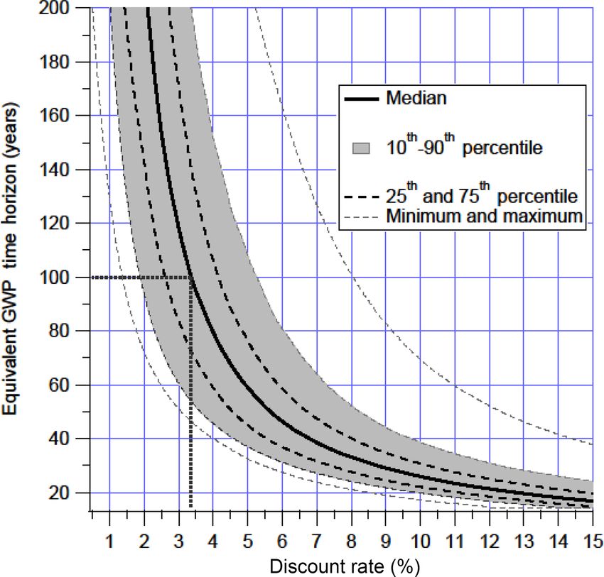
Figure 1. Impacts of emission pulses of CH4 and CO2 . Radia- Figure 2. GWP timescales consistent with discount rates based on
tive forcing (a), temperature (b), damages (c), and discounted dam- consistency of the GWP ratio with the ratio of net present damages
ages (3 %, a) for an emission pulse of 28.3 MT CH4 (10 ppb in the of CH4 and CO2 , including the interquartile and interdecile bands
first year) and 24.8 times as much CO2 emissions by mass. The un- and maximum and minimum values based on a sensitivity analysis.
derlying scenario is RCP6.0, with other parameters at their central
values.
3.2 Implying a discount rate
This analysis of evaluating the radiative forcing, temperature,
of the initial forcing, and the temperature effects decay to damages, and discounted damages of a pulse emission can be
51 % of the CO2 peak temperature (reached 18 years after used to calculate the consistent GWP timescale for a given
the pulse). The immediacy of the temperature effects for the discount rate or, conversely, the discount rates that are con-
CH4 pulse creates larger damages in both overall and dis- sistent with a given GWP timescale by comparing the net
counted dollar terms for the first 42 years. After 43 years, the present discounted marginal damages of CH4 to CO2 . Fig-
sustained CO2 effects overtake the CH4 effects. With a differ- ure 2 shows the relationship between the discount rate and
ent discount rate, a different factor would have been used to the GWP timescale. Here we focus on what discount rates are
calculate the CO2 mass used for the CO2 pulse, which would consistent with a GWP time horizon in order to show the dis-
change the crossing point for damages – a higher discount count rates implied by common choices of GWP timescales.
rate would require a larger CO2 equivalent pulse relative to The converse calculation is relevant for an audience that has a
the CH4 pulse and therefore an earlier crossing point (and preferred discount rate and is interested in the implied GWP
vice versa). Figure 1c demonstrates the dramatic increase in timescale.
damage over time due to the relationship of damage to eco- From Fig. 2, the discount rate implied by the GWP100
nomic growth. In the case of CH4 , damage peaks in 2032 is 3.3 % (interquartile range of 2.7 % to 4.1 %). The dis-
and declines until 2080 as a result of the short lifetime of the count rate implied by a 20-year GWP timescale is 12.6 %
gas. The increase in damages after 2080 is due to the com- (interquartile range of 11.1 % to 14.6 %). The results in the
ponent of the temperature response function that includes figure are truncated to the year 2300 and the calculation is
a 409-year timescale decay rate such that after 100 years truncated to the year 2500, which may matter at very low dis-
the decrease in the 1T 2 component of the damage equa- count rates due to the long lifetime of CO2 . At a 3 % discount
tion is about 0.5 % year−1 , and because that decay rate is rate, 90 % of the discounted CO2 damages from an emissions
slower than the rate of GDP growth, net damages grow. Fig- pulse comes in the first 157 years and 95 % in 189 years.
ure 1d demonstrates the dramatic decrease in future damages For CH4 , the equivalent of 90 and 95 % is 87 and 123 years,
when applying a constant discount rate. Taken as a whole, with the long tail on temperature effects causing elongated
these four figures demonstrate the trade-offs required when damages beyond the lifetime of the gas itself. Even at a 2 %
attempting to create equivalences for emissions of gases with discount rate, 95 % of the CO2 damages come in the first
very different lifetimes. 287 years. At discount rates lower than 2 %, however, trunca-
www.earth-syst-dynam.net/9/1013/2018/ Earth Syst. Dynam., 9, 1013–1024, 20181018 M. C. Sarofim and M. R. Giordano: A quantitative approach to evaluating the GWP timescale
tion effects can account for errors in damage ratio estimates Table 1. Parameter sensitivity analysis: examining the sensitivity
of greater than a percent, indicating that longer calculation of the GWP–discount rate equivalency as shown in the uncertainty
timeframes may be necessary to capture the full effect of the ranges in Fig. 2 as a function of the individual parameters of the
emissions pulse. calculation. The ratio is calculated as the ratio of the median of the
There is much discussion regarding which discount rates estimated GWPs given the highest and lowest value of each param-
eter. The results in this table are derived assuming a discount rate of
are most appropriate for use in evaluating climate damages.
3 %.
Since 2003, the US government has used discount rates of
3 % and 7 % to evaluate regulatory actions, and 3 % was Parameter Ratio of
deemed appropriate for regulation that “primarily and di- highest to lowest
rectly affects private consumption” and 7 % for regulations damages estimate
that “alter the use of capital in the private sector” (OMB,
GDP 2.07
2003). From the current analysis, a 3 % discount rate is con-
Damage exponent 1.63
sistent with a GWP of 118 years (interquartile range of 84– Scenario 1.31
171 years) and 7 % with a GWP of 38 years (interquartile Temperature offset 1.26
range of 32–47 years). The OMB Circular also recognizes Climate sensitivity 1.16
that there are special ethical considerations when impacts Forcing imbalance 1.02
may accrue to future generations, and climate change is a
prime example of an impact for which discount rates lower
than 3 % could be justified. A number of researchers have ad-
vocated for time-dependent declining discount rates (Weitz-
man, 2001; Newell and Pizer, 2003; Gollier et al., 2008). age exponent, or emissions scenario), the longer the equiva-
The UK and France both already use declining discount rates lent timescale is for a given discount rate.
in policy-making, and in both cases, the certainty equiva- While CO2 and CH4 are the largest contributors to climate
lent discount rate drops below 3 % within 100 years and ap- change (as evaluated by contributions of historical emissions
proaches 2 % within 300 years (Cropper et al., 2014). to present-day radiative forcing as in Table 8.SM.6 in the
This paper does not select a single “correct” discount rate. IPCC and by the magnitude of present-day emissions as eval-
However, the analysis shows that the 100-year timescale is uated by the standard GWP100), it is also informative to
consistent, within the interquartile range, with the 3 % dis- evaluate emissions of other gases with these techniques. Ta-
count rate that is commonly used for climate change analy- ble 2 shows five gases and their atmospheric lifetimes. For
sis. In contrast, a 20-year time horizon for the GWP implies each gas, an “optimal” GWP timescale was calculated that
discount rates larger than those used in any climate change would replicate the ratio of net present damage of that gas to
analysis publications to date. CO2 at a discount rate of 3 %. The ratio of the GWP100 and
the GWP20 to that optimal damage ratio is also shown. For
3.3 Sensitivity analyses
longer-lived gases (e.g., N2 O and HFC-23), there is no inte-
gration time period that can produce a ratio as large as the
Figure 2 shows the median, interquartile, interdecile, and ex- calculated damage ratio at a discount rate of 3 %. For these
tremes of the equivalent GWP time horizon corresponding to gases, we list the timescale that yields the maximum possible
a given discount rate from a sensitivity analysis. The uncer- ratio and note that the GWP for longer-lived gases is fairly in-
tainty was calculated assuming equal likelihood of each of sensitive to timescale (further comparisons of non-CO2 gases
the 972 combinations of all of the parameter choices used in are presented in the Supplement). This table shows that at
this paper: four RCPs, three climate sensitivities, three dam- a discount rate of 3 % and as evaluated using net present
age exponents, three forcing imbalance options, three tem- damage ratios, the use of a 100-year timescale is consistent
perature offsets, and three GDP growth rates. The ranges (interquartile range) with the optimal timescale / damage ra-
chosen for each parameter are described in the Methods sec- tios for methane. For gases with lifetimes in centuries, the
tion. The parameters with the largest effect on the uncertainty GWP at any timescale undervalues these gases, but the mag-
of the calculated GWP (at a discount rate of 3 %) are the nitude of that undervaluation is somewhat insensitive to the
rate of GDP growth and the damage exponent (see Table 1). choice of timescale. For the longest-lived gases, the GWP
For these six parameters, the choices that lead to larger dam- also undervalues reductions in these gases, but the longer the
ages from CH4 relative to CO2 are a low GDP growth, a low timescale the better the match.
damage exponent, a low-emissions scenario, a higher tem- In addition to investigating the sensitivity of these results
perature offset (e.g., assuming that damages are a function of to different choices of the six listed parameters and five
warming from preindustrial, not warming from present day), different gases, several other sensitivity experiments were
a lower climate sensitivity, and a higher current forcing im- performed. These experiments were chosen to investigate
balance. The general trend is that the more that damages are whether certain assumptions are important and alternate ap-
expected to grow in the future (e.g., high GDP growth, dam- proaches to constructing the model.
Earth Syst. Dynam., 9, 1013–1024, 2018 www.earth-syst-dynam.net/9/1013/2018/M. C. Sarofim and M. R. Giordano: A quantitative approach to evaluating the GWP timescale 1019
Table 2. Optimal timescale of non-CO2 gases. Implicit timescale evaluated for non-CO2 gases with the GWP to damage ratio for the two
most common GWP timescales. Asterisks indicate no exact match between GWP ratio and damage ratio; the closest value is given instead.
The third and fourth columns show the ratio of the GWP for a given gas to the calculated damage ratio. Interquartile uncertainty ranges are
presented for the timescale and damage ratios for CH4 . The results in this table are derived assuming a discount rate of 3 %.
Gas Lifetime Optimal GWP100 / damage GWP20 / damage
timescale ratio ratio
CH4 12.4 120 (84–172) 1.15 (1.52–0.87) 3.4 (4.49–2.57)
N2 O 121 ∗ 52 0.85 0.84
HFC-134a 13.4 115 1.11 3.2
HFC-23 222 ∗ 105 0.71 0.62
PFC-14 50 000 >400 0.62 0.45
The first set of experiments involve analysis choices that For this experiment, the Ramsey parameters were calibrated
end up having little difference in terms of timescale estima- to yield an average discount rate for the reference GDP of
tion. In general, this is because changes in these choices af- 5 % over the first 30 years of the analysis given a pure rate
fect both the GWP and the damage estimation equally and of time preference of 0.01 %. Under this assumption, the me-
therefore cancel out. One experiment involved changing the dian timescale under the reference GDP scenario increases
size of the emissions pulse to 373 MMT (about 1 year of to 135 years because even though the initial discount rates
anthropogenic emissions according to Saunois et al., 2016). are higher than 3 %, over the entire period of the analysis
The effect on damage ratios of this change was less than the average discount rate is only 1.5 %. However, unlike in
1 %. Another experiment involved doubling the radiative ef- the original analysis, under the high GDP growth scenario
ficiency of methane; while this led to a doubling of the esti- the damage ratio increases and the equivalent timescale de-
mated damage ratio, it also led to a doubling of the estimated creases to 90 years because the increase in discount rate re-
GWP such that the change in estimated timescale was about sulting from high growth has a larger effect on damages than
1/10 of 1 %. This experiment confirms that timescale esti- the long-term increase in GDP (and vice versa for low GDP
mates are insensitive to updates to estimates of the radiative growth). The difference between the damage ratios for the
efficiency of individual gases (such as the finding of Etmi- high and low GDP growth scenarios is still about a factor of
nan et al., 2016, that methane has greater forcing effects than 2. A future analysis could pair GDP scenarios with emissions
previously estimated). A third experiment arose because of scenarios to take into account the potential correlation of the
the question of consistency between the treatment of CO2 two.
and CH4 in terms of climate–carbon feedbacks (Gasser et al., Boucher (2012) and Fuglestvedt et al. (2003) both applied
2017; Sterner and Johansson, 2017). Using the CO2 lifetime similar approaches to the one used in this paper, but both pa-
from Gasser et al. (2017) without climate–carbon feedbacks, pers identified a discount rate consistent with the GWP100
an increase in damage ratios of about 8 % was estimated, but that was somewhat lower than the median 3.3 % value found
a similar increase in GWP of about 7 % was estimated, with a in this paper. The most evident difference between the ap-
net effect on timescales of less than 1 %. The converse exper- proach in these previous papers and this article is that this
iment (including climate–carbon feedbacks in both the CO2 article assumes that damages are expressed as a percent of
and CH4 lifetimes) was not analyzed due to the increased GDP, and the previous analyses did not. In order to more
complexity of the calculation. However, given that the virtue closely emulate the Boucher and Fuglestvedt approach, the
of the GWP is its simplicity, the authors suggest that the use model was tested by using constant GDP over the entire time
of lifetimes without climate–carbon feedbacks for either gas period, and the GWP100 was found to be the most consistent
should be preferred over the inclusion of those feedbacks in with a discount rate of 1.2 % (interquartile range of 1.0 % to
the lifetimes of both gases (Sarofim, 2016). 1.9 %) in contrast to 3.3 % (interquartile range of 2.7 % to
Another experiment considered the use of a Ramsey- 4.1 %).
type framework for discounting future damages. The use of Myhre et al. (2013) justified the exclusion of the 500-
such a framework has been recommended by the National year GWP based on the large uncertainties and ambiguities
Academies (NAS, 2017). In this framework, discount rates involved with far future projections. This analysis extends
are a function of the marginal utility of consumption, the through 2500 and therefore might be subject to some of those
pure rate of time preference, and the future growth rate of same uncertainties. Therefore, the effect of two shorter time
per capita consumption. It is the latter dependence that makes periods was investigated. When truncating the analysis after
this sensitivity analysis particularly interesting, as this pairs 150 years, the GWP100 was still found to be consistent with
higher consumption growth (leading to higher damage ratios) a discount rate of 3.3 %, with the upper interquartile bound
with higher discount rates (leading to lower damage ratios). also remaining constant at 4.1 %, though the lower end of the
www.earth-syst-dynam.net/9/1013/2018/ Earth Syst. Dynam., 9, 1013–1024, 20181020 M. C. Sarofim and M. R. Giordano: A quantitative approach to evaluating the GWP timescale
interquartile range decreased modestly to 2.4 %. When the ficiency and consistent treatment of climate–carbon feed-
analysis was truncated at 100 years into the future, the im- backs.
plicit discount rates dropped more substantially, to 2.6 % (in- In contrast, the timescale of ocean heat uptake, the lag
terquartile range of 1.5 % to 3.5 %). Truncating the analysis between the timing of atmospheric temperature response to
will naturally make CH4 mitigation appear more favorable forcing and the response of sea level (e.g., Zickfeld et al.,
relative to CO2 , but even discount rates as small as 3 % are 2017), and other issues that are inherent to the timing of cli-
sufficient to make effects more than 150 years into the future mate impacts – but are not necessarily included in the GWP
inconsequential to the results. calculation – might all affect the implied timescale. One po-
A final experiment considered the inclusion of damages tential way to explore some of these effects would be to use
due to rate of change and due to absolute temperature. The a more complex climate model to evaluate the radiative forc-
inclusion of rate-of-change damages has had important in- ing and temperature effects of the emission pulses. The shape
fluences on previous analyses. For example, in Manne and of the damage function can also have a substantial effect;
Richels (2001), the dynamic optimization solution for ap- different exponents for the polynomial form were tested, as
proaching a temperature threshold placed little value on CH4 was the inclusion of rate of change, but the full range of
reduction relative to CO2 until a couple decades before the possible damage functions is substantially larger, including
threshold was reached; but when a rate-of-change require- multi-polynomial behavior (Weitzman, 2001) and the poten-
ment was added, the relative value of CH4 reduction stayed tial for persistent influences on economic growth (Burke et
fairly constant over the time period. The challenge for this al., 2015).
analysis is in determining the appropriate damage form, as An additional category of effects has less relevance to an
the literature for estimating damages due to rate of change analysis of an appropriate timescale for climate impacts, but
is not as robust as for absolute changes. As a test case, the would be important for overall valuation. These are gener-
peak rate-of-change damages under the median parameter ally gas-specific effects that should most appropriately be
values were calibrated to be equal to the absolute damages considered on a case-by-case basis rather than folding into a
in the year 2060 (50 years into the analysis). The effect of timescale analysis that will influence the mitigation choices
the inclusion of this effect was to increase the damage ra- for all gases. One example is the inclusion of CO2 fertil-
tio of CH4 to CO2 by 2.4 %. This fairly modest impact is ization effects, which would reduce the relative importance
consistent with the results of Bowerman et al. (2013) and of decreasing CO2 compared to other gases. Other exam-
Rogelj et al. (2015), which suggest that near-term mitiga- ples include the health effects of O3 produced by reaction
tion of SLCFs has modest effects on reducing the peak rate of CH4 in the atmosphere (Shindell et al., 2015; Sarofim et
of change for higher future emissions scenarios and that de- al., 2017), CO2 effects on ocean acidification, and the pos-
layed SLCF mitigation may yield most of the same benefits sible reduced efficacy of CH4 compared to CO2 (Modak et
as immediate SLCF mitigation in terms of both peak absolute al., 2018). These effects can be important for making miti-
change and rate of change. In order examine how this effect gation decisions but are outside of the scope of considera-
could be sensitive to a lower emissions scenario, the analysis tion for a study focusing on how to choose a time horizon
was repeated for the RCP3PD scenario by itself. Under this for comparing climate impacts. As an example, if the solu-
assumption, the damage ratio increases by 53 %, resulting in tion to undervaluing CH4 mitigation due to its O3 effects is
a decrease in the optimal timescale for RCP3PD associated to reduce the appropriate timescale for GHG comparisons,
with a discount rate of 3 % from 94 to 54 years. This result is an identical gas without O3 chemistry implications would be
also consistent with Bowerman et al., who found more bene- similarly prioritized. One potential approach that could be
fit in reducing near-term SLCF emissions if future emissions explored might be to apply a multiplier to the GWP after cal-
are expected to be low. culation to take into account these non-climatic effects, much
like the GWP of methane takes into account indirect effects
3.4 Additional uncertainties
on climate through the production of tropospheric O3 and
stratospheric H2 O by the use of a multiplicative factor.
There are a number of uncertainties involved in this anal-
ysis. They can be divided into three categories: those that 3.5 Caveats
may change the relative climate-related discounted damages
of CH4 compared to CO2 but have minimal effect on the im- The analysis presented here suggests that the use of a 100-
plied timescale of the GWP, those that have a large impact on year time horizon for the GWP is in good agreement with
the implied timescale, and those effects of CH4 and CO2 that what many consider an appropriate discount rate; however,
are unrelated to their climate forcing. we offer several caveats. Most importantly, this analysis
As shown above, uncertainties in this analysis that do not makes the assumption that the net present damage of CH4
have a large impact on the calculated GWP timescale in- and CO2 is the best metric for evaluating the relative impact
clude factors that have similar effects on the GWP and the of gases. When analyzing several different common metrics,
CH4 : CO2 discounted damage ratio, such as radiative ef- Azar and Johansson (2012) asked whether society would pre-
Earth Syst. Dynam., 9, 1013–1024, 2018 www.earth-syst-dynam.net/9/1013/2018/M. C. Sarofim and M. R. Giordano: A quantitative approach to evaluating the GWP timescale 1021
fer integrated metrics such as the GWP, single time period sistent with a 3 % discount rate to 54 years. Applying the
metrics such as the GTP, or economic metrics such as the methodology in this paper to calculate the implied intertem-
global damage potential, which is parallel to the metric given poral values of a 20-year GWP, a timescale that has received
primary weight in this paper. Considering the applications of some recent attention, results in an implicit discount rate of
a metric within the context of an integrated assessment model 12.6 % (interquartile range of 11.1 % to 14.6 %).
could enable the analysis of more complex economic inter- These results provide support for the contention that
actions. Alternatively, a decision-making framework might 100 years is a reasonable timescale choice for the GWP given
consider factors other than damages; for example, in a multi- the assumption that the relative climate damage of pulses of
stage decision-making process under uncertainty, it might be different greenhouse gases is an appropriate means of valu-
possible that long-lived gas mitigation should be prioritized ation and that the 3 % discount rate is a reasonable measure
in order to increase future option value. Or there might be of the value of the future. This finding is robust to a num-
reasons to prioritize mitigation options that apply to capital ber of sensitivity analyses. In contrast, the analysis suggests
stocks with long lifetimes or to decisions that involve path that the 20-year GWP timescale is the most consistent with
dependence, as those decisions would be more costly to re- an implicit discount rate much higher than the standard so-
verse in the future. cial discount rate, except in scenarios with low future emis-
This metric approach is also not designed to achieve a sions and high rate-of-change damages, similar to concerns
long-term temperature goal such as stabilization at 2 ◦ C expressed in other analyses (Shoemaker and Schrag, 2013).
above preindustrial temperatures. We note that no metric de- However, while the implicit timescale was derived from ana-
signed to trade off emission pulses is consistent with stabi- lyzing the climate impacts resulting from CH4 emissions rel-
lization. One solution to this dilemma is the GWP∗ intro- ative to CO2 climate impacts, the results do not necessarily
duced by Allen et al. (2016), which creates an equivalence inform a specific relative importance of CH4 mitigation com-
between an emission pulse of CO2 and a constant stream of pared to CO2 . Such a relative importance calculation should
CH4 . This analysis only looks at a pulse of emissions in 2011 take into account the latest research on radiative efficiencies
and does not examine whether the equivalent timescale might (Etminan et al., 2016) and could potentially also take into
change over time. account non-climate impacts like the health effects of CH4 -
derived O3 (Shindell, 2015; Sarofim et al., 2017). The inclu-
sion of non-climate impacts could perhaps use an adjustment
4 Conclusions factor in the same way that the CH4 GWP already includes
adjustment factors for the climate effects of CH4 -derived O3 .
This analysis uses a global damage potential approach to cal- Additionally, the appropriate GWP timescales can also be in-
culate the implicit discount rate corresponding to different formed by the manner in which the metric is being used for
GWP timescales. While this is not the first analysis to calcu- policy or informational purposes.
late the implicit discount rate of the 100-year GWP (Boucher, The methodology presented here is transparent (the code
2012; Fuglestvedt et al., 2003), the framework presented here is available in the Supplement), rigorous (the parameters
allows for a more complete and wide-ranging analysis of sen- and functional forms are derived from respected sources),
sitivities than has been presented previously, and the connec- and flexible (as demonstrated by a wide range of sensitiv-
tion between the timescale and the implicit discount rate is ity analyses from the inclusion of rate-of-change damages
made more clearly. The 100-year GWP is the inter-gas com- to Ramsey discounting). This framework can be a valuable
parison metric with the widest use, and the results presented resource for quantitatively examining appropriate timescales
here show that the 100-year timescale is consistent with an given different assumptions about discounting, the relation-
implied discount rate of 3.3 % (interquartile range of 2.7 % ship of damages to both absolute and rate of temperature
to 4.1 %). Alternatively, the 3 % discount rate used for cal- changes, tipping points, future emissions scenarios, and other
culating social damages in some regulatory impact analysis factors.
contexts is consistent with timescales of 84–171 years. The
uncertainty range in the results is the most sensitive to as-
sumptions regarding future GDP growth and to the choice Code availability. The R code used in developing this paper can
of exponent in the damage function. These results are in- be found in the Supplement.
sensitive to assumptions regarding radiative efficiency, pulse
size, and consistent treatment of climate–carbon feedbacks.
At discount rates of 3 % or higher, the analysis can be trun-
cated to 150 years (rather than the default calculation through
2500) with little effect. The inclusion of damages resulting The Supplement related to this article is available online
from the rate of change in addition to absolute temperature at https://doi.org/10.5194/esd-9-1013-2018-supplement.
changes has little effect except in the case of a low-emissions
future, for which it results in a decrease in the timescale con-
www.earth-syst-dynam.net/9/1013/2018/ Earth Syst. Dynam., 9, 1013–1024, 20181022 M. C. Sarofim and M. R. Giordano: A quantitative approach to evaluating the GWP timescale
Author contributions. Both MCS and MRG contributed to ex- Chang-Ke, W., Xin-Zheng, L., and Hua, Z.: Shares Differences of
periment design, coding, figure development, and paper writing. Greenhouse Gas Emissions Calculated with GTP and GWP for
Major Countries, Advances in Climate Change Research, 4, 127–
132, 2013.
Competing interests. The authors declare that they have no con- Christensen, P., Gillingham, K., and Nordhaus, W.: Uncertainty in
flict of interest. forecasts of long-run economic growth, P. Natl. Acad. Sci. USA,
115, 5409–5414, 2018.
Cropper, M. L., Freeman, M. C., Groom, B., and Pizer, W. A.: De-
Disclaimer. This publication was developed under assistance clining discount rates, American Economic Review: Papers and
agreement no. X3-83588701 awarded by the U.S. Environmental Proceedings, 104, 538–543, 2014.
Protection Agency to AAAS. It has not been formally reviewed by Daniel, J. S., Solomon, S., Sanford, T. J., McFarland, M., Fu-
the EPA. The views expressed in this document are solely those of glestvedt, J. S., and Friedlingstein, P.: Limitations of single-
the authors and do not necessarily reflect those of the agency. The basket trading: lessons from the Montreal Protocol for climate
EPA does not endorse any products or commercial services men- policy, Climatic Change, 111, 241–248, 2012.
tioned in this publication. De Cara, S., Debove, E., and Jayet, P. A.: Global Warming Po-
tentials: Imperfect but second-best metric for climate change,
unpublished, available at: http://stephane.decara.free.fr/mypdf/
DeboDeCaJaye05b.pdf (last access: 14 August 2018), 2005.
Acknowledgements. Michael R. Giordano was supported as a
Dell, M., Jones, B. F., and Olken, B. A.: Temperature Shocks and
Science and Technology Policy Fellow by the American Associa-
Economic Growth: Evidence from the Last Half Century, Am.
tion for the Advancement of Science (AAAS) STPF program. The
Econ. J.-Marcoecon., 4, 66–95, 2012.
authors would like to thank numerous colleagues at the EPA for
Deuber, O., Luderer, G., and Edenhofer, O.: Physico-
their thoughts and discussions regarding GHG metrics and climate
economic evaluation of climate metrics: A concep-
economics.
tual framework, Environ. Sci. Policy, 29, 37–45,
https://doi.org/10.1016/j.envsci.2013.01.018, 2013.
Edited by: Daniel Kirk-Davidoff
Edwards, M. R. and Trancik, J. E.: Climate impacts of energy tech-
Reviewed by: William Collins and three anonymous referees
nologies depend on emissions timing, Nat. Clim. Change, 4,
347–352, 2014.
Edwards, M. R., McNerney, J., and Trancik, J. E.: Testing emissions
References equivalency metrics against climate policy goals, Environ. Sci.
Policy, 66, 191–198, 2016.
Allen, M. R., Fuglestvedt, J. S., Shine, K. P., Reisinger, A., Pierre- Etminan, M., Myhre, G., Highwood, E. J., and Shine, K. P.: Radia-
humbert, R. T., and Forster, P. M.: New use of global warming tive forcing of carbon dioxide, methane, and nitrous oxide: A sig-
potentials to compare cumulative and short-lived climate pollu- nificant revision of the methane radiative forcing, Geophys. Res.
tants, Nat. Clim. Change, 6, 773–776, 2016. Lett., 43, 12614–12623, https://doi.org/10.1002/2016GL071930,
Alvarez, R. A., Pacala, S. W., Winebrake, J. J., Chameides, W. L., 2016.
and Hamburg, S. P.: Greater focus needed on methane leakage Fuglestvedt, J. S., Berntsen, T. K., Godal, O., Sausen, R., Shine, K.
from natural gas infrastructure, P. Natl. Acad. Sci. USA, 109, P., and Skodvin, T.: Metrics of climate change: Assessing radia-
6435–6440, https://doi.org/10.1073/pnas.1202407109, 2012. tive forcing and emission indices, Climatic Change, 58, 267–331,
Azar, C. and Johansson, D. J. A.: On the relationship be- 2003.
tween metrics to compare greenhouse gases – the case of Gasser, T., Peters, G. P., Fuglestvedt, J. S., Collins, W. J., Shin-
IGTP, GWP and SGTP, Earth Syst. Dynam., 3, 139–147, dell, D. T., and Ciais, P.: Accounting for the climate-carbon
https://doi.org/10.5194/esd-3-139-2012, 2012. feedback in emission metrics, Earth Syst. Dynam., 8, 235–253,
Böhringer, C., Löschel, A., and Rutherford, T. F.: Efficiency gains https://doi.org/10.5194/esd-8-235-2017, 2017.
from “what”-flexibility in climate policy an integrated CGE as- GISTEMP team: GISS Surface temperature analysis (GISTEMP),
sessment, Energ. J., 0, 405–424, 2006. NASA Goddard Institute for Space Studies, available at: https://
Boucher, O.: Comparison of physically- and economically-based data.giss.nasa.gov/gistemp/tabledata_v3/GLB.Ts+dSST.txt (last
CO2 -equivalences for methane, Earth Syst. Dynam., 3, 49–61, access: 4 August 2017), 2017.
https://doi.org/10.5194/esd-3-49-2012, 2012 Gollier, C., Koundouri, P., and Pantelidis, T.: Declining discount
Bowerman, N. H., Frame, D. J., Huntingford, C., Lowe, J. A., rates: Economic justifications and implications for long-run pol-
Smith, S. M., and Allen, M. R.: The role of short-lived climate icy, Econ. Policy, 23, 758–795, 2008.
pollutants in meeting temperature goals, Nat. Clim. Change, 3, Howarth, R. W., Santoro, R., and Ingraffea, A.: Methane and the
1021–1024, 2013. greenhouse-gas footprint of natural gas from shale formations,
Brazil INDC: Brazil’s Intended Nationally Determined Contribu- Climatic Change, 106, 679–690, https://doi.org/10.1007/s10584-
tion: Federative Republic of Brazil, available at: http://www4. 011-0061-5, 2011.
unfccc.int/submissions/INDC (last access: 14 August 2018), Howarth, R., Santoro, R., and Ingraffea, A.: Venting and leaking of
2015. methane from shale gas development: response to Cathles et al.,
Burke, M., Hsiang, S. M., and Miguel, E.: Global non-linear effect Climatic Change, 113, 537–549, 2012.
of temperature on economic production, Nature, 527, 235–239,
2015.
Earth Syst. Dynam., 9, 1013–1024, 2018 www.earth-syst-dynam.net/9/1013/2018/M. C. Sarofim and M. R. Giordano: A quantitative approach to evaluating the GWP timescale 1023 Hsiang, S., Kopp, R., Jina, A., Rising, J., Delgado, M., Mohan, S., Ocko, I. B., Hamburg, S. P., Jacob, D. J., Keith, D. W., Keohane, Rasmussen, D. J., Muir-Wood, R., Wilson, P., Oppenheimer, M., N. O., Oppenheimer, M., Roy-Mayhew, J. D., Schrag, D. P., and Larsen, K., and Houser, T.: Estimating economic damage from Pacala, S. W.: Unmask temporal trade-offs in climate policy de- climate change in the United States, Science, 356, 1362–1369, bates, Science, 356, 492–493, 2017. 2017. OMB: Office of Management and Budget: Circular A-4, available Jackson, S. C.: Parallel pursuit of near-term and long-term climate at: https://www.whitehouse.gov/sites/whitehouse.gov/files/omb/ mitigation, Science, 326, 526–527, 2009. circulars/A4/a-4.pdf (last access: 14 August 2018), 2003. Johansson, D. J.: Economics-and physical-based metrics for com- Reisinger, A., Meinshausen, M., and Manning, M.: Future paring greenhouse gases, Climatic Change, 110, 123–141, 2012. changes in global warming potentials under representa- Jørgensen, S. V., Hauschild, M. Z., and Nielsen, P. H.: Assessment tive concentration pathways, Environ. Res. Lett, 6, 1–8, of urgent impacts of greenhouse gas emissions – the climate tip- https://doi.org/10.1088/1748-9326/6/2/024020, 2011. ping potential (CTP), Int. J. Life Cycle Ass., 19, 919–930, 2014. Reisinger, A., Havlik, P., Riahi, K., van Vliet, O., Obersteiner, M., Lashof, D. A. and Ahuja, D. R.: Relative contributions of green- and Herrero, M.: Implications of alternative metrics for global house gas emissions to global warming, Nature, 344, 529–531, mitigation costs and greenhouse gas emissions from agriculture, 1990. Climatic Change, 117, 677–690, 2013. Mallapragada, D. and Mignone, B. K.: A consistent concep- Rodhe, H.: A comparison of the contribution of various tual framework for applying climate metrics in technol- gases to the greenhouse effect, Science, 248, 1217–1219, ogy life cycle assessment, Environ. Res. Lett., 12, 1–10, https://doi.org/10.1126/science.248.4960.1217, 1990. https://doi.org/10.1088/1748-9326/aa7397, 2017. Rogelj, J., Meinshausen, M., Schaeffer, M., Knutti, R., and Riahi, Manne, A. S. and Richels, R. G.: An alternative approach to es- K.: Impact of short-lived non-CO2 mitigation on carbon budgets tablishing trade-offs among greenhouse gases, Nature, 410, 675– for stabilizing global warming, Environ. Res. Lett., 10, 1–10, 677, 2001. 075001, https://doi.org/10.1088/1748-9326/10/7/075001, 2015. Manne, A. S. and Richels, R. G.: The role of non-CO2 greenhouse Sarofim, M., Forest, C., Reiner, D., and Reilly, J.: Stabilization gases and carbon sinks in meeting climate objectives, Energ. J., and global climate change, Global Planet. Change, 47, 266–272, Special Issue, 393–404, 2006. 2005. Medhaug, I., Stolpe, M. B., Fischer, E. M., and Knutti, R.: Recon- Sarofim, M. C.: The GTP of methane: modeling analysis ciling controversies about the “global warming hiatus”, Nature, of temperature impacts of methane and carbon diox- 545, 41–47, 2017. ide reductions, Environ. Model. Assess., 17, 231–239, Modak A., Bala, G., Caldeira, K., and Cao, L.: Does shortwave ab- https://doi.org/10.1007/s10666-011-9287-x, 2012. sorption by methane influence its effectiveness?, Clim. Dynam., Sarofim, M. C.: Interactive comment on “Accounting for 1–20, https://doi.org/10.1007/s00382-018-4102-x, 2018. the climate-carbon feedback in emissions metrics” by Moore, F. and Diaz, D. B.: Temperature impacts on economic Thomas Gasser et al., Earth Syst. Dynam. Discuss., growth warrant stringent mitigation policy, Nat. Clim. Change, https://doi.org/10.5194/esd-2016-55-SC1, 2016. 5, 127–131, https://doi.org/10.1038/nclimate2481, 2015. Sarofim, M. C., Waldhoff, S. T., and Anenberg, S. C.: Valuing the Myhre, G., Shindell, D., Bréon, F.-M., Collins, W., Fuglestvedt, Ozone-Related Health Benefits of Methane Emission Controls, J., Huang, J., Koch, D., Lamarque, J.-F., Lee, D., Mendoza, Environ. Resour. Econ., 66, 45–63, 2017. B., Nakajima, T., Robock, A., Stephens, G., Takemura, T., and Saunois, M., Jackson, R. B., Bousquet, P., Poulter, B., and Zhang, H.: Anthropogenic and Natural Radiative Forcing, in: Canadell, J. G.: The growing role of methane in anthro- Climate Change 2013: The Physical Science Basis. Contribu- pogenic climate change, Environ. Res. Lett., 11, 120207, tion of Working Group I to the Fifth Assessment Report of https://doi.org/10.1088/1748-9326/11/12/120207, 2016. the Intergovernmental Panel on Climate Change, edited by: Schmalensee, R.: Comparing Greenhouse Gases for Policy Pur- Stocker, T. F., Qin, D., Plattner, G.-K., Tignor, M., Allen, S. poses, Energ. J., 14, 245–255, 1993. K., Boschung, J., Nauels, A., Xia, Y., Bex, V., and Midgley, Shindell, D. T.: The social cost of atmospheric release, Climatic P. M., Cambridge University Press, Cambridge, United King- Change, 130, 313–326, 2015. dom and New York, NY, USA, 659–740, https://doi.org/10.1017/ Shindell, D., Borgford-Parnell, N., Brauer, M., Haines, A., Kuylen- CBO9781107415324.018, 2013. stierna, J. C., Leonard, S. A., Ramanathan, V., Ravishankara, A., NAS: National Academies of Sciences, Engineering, and Amann, M., and Srivastava, L.: A climate policy pathway for Medicine: Valuing Climate Damages: Updating Estima- near-and long-term benefits, Science, 356, 493–494, 2017. tion of the Social Cost of Carbon Dioxide, available at: Shine, K. P., Fuglestvedt, J., Hailemariam, K., and Stuber, N.: Al- https://www.nap.edu/catalog/24651/valuing-climate-damages- ternatives to the global warming potential for comparing climate updating-estimation-of-the-social-cost-of (last access: 14 Au- impacts of emissions of greenhouse gases, Climatic Change, 68, gust 2018), 2017. 281–302, https://doi.org/10.1007/s10584-005-1146-9, 2005. Newell, R. G. and Pizer, W. A.: Discounting the distant future: how Shoemaker, J. K. and Schrag, D. P.: The danger of overvaluing much do uncertain rates increase valuations?, J. Environ. Econ. methane’s influence on future climate change, Climatic Change, Manag., 46, 52–71, 2003. 120, 903–914, 2013. Nordhaus, W. D.: Evolution of Assessments of the Economics of Smith, S. M., Lowe, J. A., Bowerman, N. H. A., Gohar, L. K., Global Warming: Changes in the DICE model, 1992–2017, No. Huntingford, C., and Allen, M. R.: Equivalence of greenhouse w23319, National Bureau of Economic Research, Cambridge, gas emissions for peak temperature limits, Nat. Clim. Change, 2, MA, USA, 2017. 535–538, https://doi.org/10.1038/NCLIMATE1496, 2012. www.earth-syst-dynam.net/9/1013/2018/ Earth Syst. Dynam., 9, 1013–1024, 2018
You can also read