Understanding drivers of glacier-length variability over the last millennium
←
→
Page content transcription
If your browser does not render page correctly, please read the page content below
The Cryosphere, 15, 1645–1662, 2021
https://doi.org/10.5194/tc-15-1645-2021
© Author(s) 2021. This work is distributed under
the Creative Commons Attribution 4.0 License.

Understanding drivers of glacier-length variability
over the last millennium
Alan Huston1 , Nicholas Siler1 , Gerard H. Roe2 , Erin Pettit1 , and Nathan J. Steiger3,4
1 College  of Earth, Ocean, and Atmospheric Sciences, Oregon State University, Corvallis, OR, USA
2 Department    of Earth and Space Sciences, University of Washington, Seattle, WA, USA
3 Institute of Earth Sciences, Hebrew University, Jerusalem, Israel
4 Lamont-Doherty Earth Observatory, Columbia University, Palisades, NY, USA

Correspondence: Nicholas Siler (nick.siler@oregonstate.edu)

Received: 11 August 2020 – Discussion started: 28 August 2020
Revised: 10 February 2021 – Accepted: 19 February 2021 – Published: 1 April 2021

Abstract. Changes in glacier length reflect the integrated        1   Introduction
response to local fluctuations in temperature and precipi-
tation resulting from both external forcing (e.g., volcanic       The length of a glacier reflects both its topographic and cli-
eruptions or anthropogenic CO2 ) and internal climate vari-       mate setting and arises from a balance between accumulation
ability. In order to interpret the climate history reflected in   (mass gain) and ablation (mass loss), mediated by the catch-
the glacier moraine record, the influence of both sources of      ment geometry and the dynamics of ice flow. Past fluctua-
climate variability must therefore be considered. Here we         tions in glacier length often leave moraines on the landscape.
study the last millennium of glacier-length variability across    If the age of these moraines can be determined, they be-
the globe using a simple dynamic glacier model, which we          come valuable proxies of past climate change (e.g., Solomina
force with temperature and precipitation time series from a       et al., 2015). The decadal-and-longer response time of glacier
13-member ensemble of simulations from a global climate           length means that glaciers act as low-pass filters of climate
model. The ensemble allows us to quantify the contributions       and thereby have the potential to reveal climate trends that
to glacier-length variability from external forcing (given by     would otherwise go undetected (Balco, 2009).
the ensemble mean) and internal variability (given by the            Changes in climate can arise from three factors: first, nat-
ensemble spread). Within this framework, we find that in-         ural climate forcings, such as solar luminosity, variations in
ternal variability is the predominant source of length fluc-      the Earth’s orbit, and volcanic eruptions that alter the fluxes
tuations for glaciers with a shorter response time (less than     of energy entering or leaving the climate system; second,
a few decades). However, for glaciers with longer response        anthropogenic forcing, such as emissions of CO2 and in-
timescales (more than a few decades) external forcing has         dustrial aerosols, that also affect Earth’s energy budget; and
a greater influence than internal variability. We further find    third, the internal climate variability that would occur in the
that external forcing also dominates when the response of         atmosphere–ocean–cryosphere system even under constant
glaciers from widely separated regions is averaged. Single-       external conditions. Internal variability can be thought of as
forcing simulations indicate that, for this climate model,        the year-to-year fluctuations that happen due to the chaotic
most of the forced response over the last millennium, pre-        nature of atmospheric and oceanic dynamics. It can exhibit
anthropogenic warming, has been driven by global-scale            some degree of interannual persistence due to the longer-
temperature change associated with volcanic aerosols.             timescale components of the system (see Burke and Roe,
                                                                  2014, for a discussion in the context of glaciers).
                                                                     Our primary focus in this study is on the relative impor-
                                                                  tance of forced and unforced climate variability for glacier
                                                                  fluctuations in the pre-industrial era. We focus on the pre-
                                                                  industrial era because of its importance in interpreting the

Published by Copernicus Publications on behalf of the European Geosciences Union.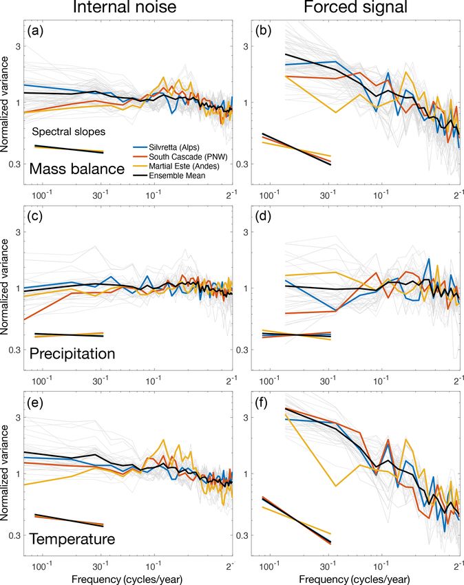
1646                                                                       A. Huston et al.: Last millennium glacier variability

Holocene glacier record. Secondly, for the industrial era           been used before in the context of glaciers in Anderson et al.
(since about 1880 or so), the central estimate of the warming       (2014) and Roe et al. (2017).
from anthropogenic forcing is 100 % of the observed warm-              We begin by applying the glacier model to three widely
ing, both globally and regionally (Haustein et al., 2019). This     separated locations with different climatic settings. The anal-
implies that both the observed industrial-era mass loss (Roe        yses highlight the importance of glacier response time: short-
et al., 2020) and retreat (Roe et al., 2017) of Alpine glaciers     response-time (i.e., less than a few decades) glaciers have
is overwhelmingly anthropogenic in origin.                          uncorrelated length fluctuations driven predominantly by re-
   Until recently, variability in glacier length over the pre-      gional, internal climate variability (a low SNR), whereas
industrial Holocene was mostly attributed to natural forcing        longer-response-time glaciers respond coherently to external
of temperature. For example, Crowley (2000) estimated that          changes in climate forcing, predominantly associated with
40 to 65 % of pre-industrial decadal-scale temperature vari-        volcanic forcing (a high SNR). Finally, we extend our anal-
ations were a result of changes in solar irradiance and vol-        yses to a global network of 76 well-observed glaciers to as-
canism. Similarly, Miller et al. (2012) have argued that the        sess the coherence of glacier response among, and within,
Little Ice Age period between approximately 1300 and 1850           individual glacierized regions.
was caused by a sequence of volcanic eruptions, with the
cooling effects of explosive volcanism made more persistent
by sea-ice–ocean feedbacks operating long after the volcanic        2     Quantifying forced and internal climate variability
aerosols were removed from the atmosphere.                                over the last millennium
   However, recent studies have shown that large variabil-
                                                                    We analyze climate variability in the Community Earth Sys-
ity in glacier length can also occur in an unforced, statisti-
                                                                    tem Model (CESM) Last Millennium Ensemble (LME).
cally constant climate due to internal climate variability (e.g.,
                                                                    The LME comprises 13 simulations that span 850–2005 CE
Oerlemans, 2000). By studying glaciers around Mt. Baker in
                                                                    (Otto-Bliesner et al., 2016). Each simulation includes the
Washington state, for example, Roe and O’Neal (2009) found
                                                                    same radiative forcing contributions from volcanic aerosols,
that internal variability alone can produce kilometer-scale ex-
                                                                    solar irradiance, orbital changes, greenhouse gases, and
cursions in glacier length on multi-decadal and centennial
                                                                    ozone aerosols, based on forcing reconstructions from the
timescales. This result highlights the importance of consid-
                                                                    fifth-generation Coupled Model Intercomparison Project
ering internal variability in addition to forced climate change
                                                                    (CMIP5; Schmidt et al., 2011). The ensemble members all
as a potential cause of past variations in glacier length. Until
                                                                    have exactly the same physics and differ only in their initial
now, however, no systematic assessment of the relative im-
                                                                    conditions. Chaotic internal dynamics and the different ini-
portance of forced versus internal variability has been con-
                                                                    tial conditions cause a spread among the ensemble members.
ducted.
                                                                    Hence, the mean of the ensemble is an estimate of the forced
   Both the local magnitude and the spatial coherence of
                                                                    climate response, while the spread among ensemble mem-
glacier-length variability have been studied for specific re-
                                                                    bers represents internal climate variability (e.g., Deser et al.,
gions using existing observations. For example, there is a
                                                                    2012).
notable inter-hemispheric disparity in the timing of the max-
                                                                       For the first part of our analysis, we focus on three geo-
imum ice extent during the Holocene for glaciers in New
                                                                    graphically diverse glaciers, with distinct climatic settings:
Zealand versus the Alps (Schaefer et al., 2009). Addition-
                                                                    (i) the Silvretta glacier in the Alps, (ii) the South Cascade
ally, mid-to-late Holocene glacier fluctuations were neither
                                                                    glacier in the American Pacific Northwest, and (iii) the Mar-
in phase nor in strict anti-phase between the hemispheres,
                                                                    tial Este glacier in the Patagonian Andes. Each of these
suggesting that regional climate variability has played an im-
                                                                    has good observations of its mass balance over the last few
portant role (Schaefer et al., 2009). Indeed, the very idea of
                                                                    decades (Medwedeff and Roe, 2017, and Table A1).
a global-scale Little Ice Age or Medieval Climate Anomaly
                                                                       We identify the grid points in the CESM model that are
has been called into question (Neukom et al., 2019).
                                                                    closest to each glacier. From the archived model output at
   We evaluate the relative importance of forced and unforced
                                                                    each of these grid points, we compute time series of aver-
climate variability on driving glacier-length fluctuations us-
                                                                    age winter precipitation (P ) and summer temperature (T ).
ing two primary research tools. The first is an archive of en-
                                                                    For grid points in the Northern Hemisphere, P is taken from
semble simulations of a global climate model, from which
                                                                    October–March and T is taken from April–September. The
we make estimates of the forced and unforced components
                                                                    seasons are flipped for grid points in the Southern Hemi-
of the climate variability, as well as the impact of each type
                                                                    sphere. We then estimate mass-balance variability using the
of climate forcing. The second is a simple dynamical glacier
                                                                    following linear approximations:
model whose parameters can be adjusted to different climate
                                                                     0
settings and glacier geometries. We measure the relative im-        bw = αP 0                                                    (1)
portance of forced and unforced variability using the signal-
                                                                    and
to-noise ratio (SNR, defined in the next section), which has
                                                                    bs0 = −λT 0 ,                                                (2)

The Cryosphere, 15, 1645–1662, 2021                                                     https://doi.org/10.5194/tc-15-1645-2021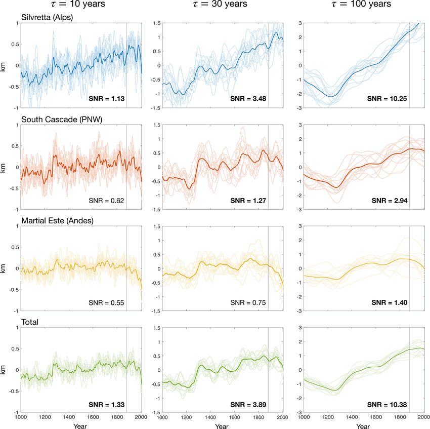
A. Huston et al.: Last millennium glacier variability 1647
where bw and bs represent winter and summer mass balance, significant at the 99 % confidence level (see Appendix). SNR
α and λ are positive constants, and primes indicate anomalies values are listed in Fig. 1 for each time series and time pe-
relative to the millennial average (1000–1999). Note that the riod, with bold font indicating statistical significance.
negative sign in Eq. (2) reflects an anticorrelation between In the winter (Fig. 1a), there is little evidence of a forced
mass balance and temperature in the summer. signal in bw0 at any glacier during either time period, as in-
Like most global climate models (GCMs), the grid resolu- dicated by SNR values that are uniformly low and in most
tion of the LME is too coarse to capture the full influence of cases statistically insignificant. This implies that interannual
orography on P and T at most glacier locations. To compen- variability in winter mass balance (and thus winter precipita-
sate for this, we choose values of α and λ for each glacier that tion) at these glaciers is dominated by internal climate noise.
produce variances in bw 0 and b0 that match the observed val- This finding is expected based on past studies of the contribu-
s
ues reported by Medwedeff and Roe (2017). This is achieved tion from winter precipitation trends in glacier change (e.g.,
by setting Medwedeff and Roe, 2017).
σb,w In contrast, bs0 shows clear evidence of a forced signal
α= (3) (Fig. 1b). During the pre-industrial period, all locations ex-
σP
hibit several abrupt spikes associated with volcanic erup-
and tions, with the most notable event being the Samalas eruption
σb,s in 1257 (e.g., Guillet et al., 2017). The amplitude of these
λ= , (4) spikes is strongest in Europe and North America, where they
σT
occur against the backdrop of a longer-term increase in bs0
where the numerators represent the observed standard devi- associated with a cooling trend that persists through the end
ations in winter and summer mass balance, and the denom- of the 19th century. Although the forced signal is statistically
inators represent the standard deviations in winter precipita- significant at all locations during the pre-industrial period,
tion and summer temperature. Annual mass-balance anoma- SNR values are less than 0.2, implying that internal noise
lies, b0 , are then equal to the sum of the summer and winter still accounts for the majority of local year-to-year tempera-
anomalies: ture variability.
Around 1900, bs0 begins to decrease at all three glaciers
b0 = bw
0
+ bs0 . (5)
in response to global warming (Fig. 1b). SNR values are
Figure 1 shows the mass-balance time series created in this greater in this period than in the pre-industrial period, re-
way. Their average is shown in the lowest panels. The vertical flecting the unprecedented strength and persistence of an-
gray line at the year 1880 marks the approximate transition thropogenic forcing. Comparing the simulated trends in bs0
from the pre-industrial era to the modern era, after which the over the 20th century with those derived from observed tem-
time axis on each panel is dilated by a factor of 4 to enhance peratures (Fig. 1b; colored vs. black lines), we find good
visibility. Figure 1 also shows bs0 calculated from observed agreement at South Cascade and Martial Este but not at Sil-
temperature anomalies (NASA GISS dataset; Lenssen et al., vretta, where the decrease in bs0 in the LME ensemble mean
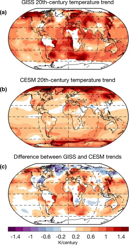
2019). is too low by 0.07 m per decade, reflecting a local warm-
The importance of the external forcing relative to the in- ing trend that is too low by 0.063 K per decade (Eq. 2, with
ternal variability can be measured by a signal-to-noise ratio λ = 1.11 m/K). One possible interpretation of this difference
(SNR), which we define as is that part of the observed warming trend at Silvretta was
the result of internal variability. This conclusion is supported
Var[b0 (t)] by the fact that the observed trend at Silvretta lies within
SNR = , (6)
Var[b0 (t)] − Var[b0 (t)] the ensemble range of simulated trends. On the other hand,
20th-century warming trends in the LME are weaker than
where Var[b0 (t)] is the variance of the ensemble mean observed trends over most of the globe (Fig. A1), suggesting
time series (i.e., the “signal” of the forced response), and that model bias likely also plays a role. We consider possible
Var[b0 (t)] is the total variance across all ensemble members causes of this bias in Sect. 3.4 but note that it does not affect
(i.e., as if all 13 time series were concatenated into a single the bulk of our analysis.
time series). The difference between the two quantities in the Finally, variability in b0 (Fig. 1c) shows the influence of
denominator represents the variance due to internal climate both bw 0 and b0 , but in different proportions for each glacier.
s
variability (i.e., the “noise”). In general, SNR values less than For example, at South Cascade glacier (red), the variance in
one indicate that most of the variance in a time series can be bw0 is a factor of 2 greater than the variance in b0 and thus
s
attributed to internal variability, while SNR values greater exerts a much stronger influence on b0 . Because bw 0 is essen-
than one indicate that most variance is driven by external tially noise, the SNR of b0 at South Cascade glacier is statisti-
forcing. For a 13-member ensemble, SNR values greater than cally insignificant in the modern era, even though bs0 contains
0.125 in the modern era or 0.098 in the pre-industrial era in- a significant forced signal. This masking of forced variance
dicate that a forced signal can be detected and is statistically in b0 by large internal variance in bw 0 despite the presence of
https://doi.org/10.5194/tc-15-1645-2021 The Cryosphere, 15, 1645–1662, 2021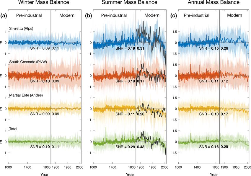
1648                                                                          A. Huston et al.: Last millennium glacier variability

Figure 1. One thousand years of mass-balance anomalies modeled using the LME output, for three different locations. (a) Winter mass
balance, (b) summer mass balance, and (c) annual mass balance in the Alps (blue), the Pacific Northwest (red), and the Patagonian Andes
(yellow), along with their average (green). Heavy colors represent the ensemble mean, while lighter colors represent individual ensemble
members. The vertical gray line at the year 1880 marks the approximate transition from the pre-industrial era to the modern era, after which
the time axis on each panel is dilated by a factor of 4 to enhance visibility. To evaluate the accuracy of LME temperatures over the modern
era, we also plot values of bs0 calculated from the observational NASA-GISS surface temperature data set in black. SNR values are given for
each glacier and era, with bold font indicating statistical significance (99 % confidence; see Appendix).

forced variance in bs0 is typical of maritime glaciers and de-          3   Glacier simulations
tailed, for example, in Young et al. (2020). At Silvretta and
Martial Este, by contrast, the variance comes mostly from               The implications of this climate variability for fluctuations
bs0 . Thus, while bw0 remains a source of noise, its amplitude          in glacier length are evaluated using the three-stage linear
is small enough that the forced signal from bs0 can still be            model of Roe and Baker (2014), which has been shown to
detected in b0 .                                                        better capture the high-frequency response of glacier dy-
     A last point to emphasize from Fig. 1 relates to the av-           namics than earlier low-order models (Harrison and Post,
eraged time series among the three glaciers (green lines).              2003; Oerlemans, 2000, 2005). The three stages, which can
These exhibit higher SNRs in bs0 and b0 than in any indi-               be diagnosed from ice dynamics in numerical models, are
vidual glacier: spatial averaging suppresses noise and brings           (1) changes in interior thickness, which drive (2) changes in
out a common forced signal. This echoes results from studies            terminus ice flux, which in turn drive (3) changes in glacier
of modern-day warming, which have found that the anthro-                length. Collectively, the three stages can be represented as a
pogenic signal is clearest at global scales, even when it is            linear, third-order differential equation,
obscured by internal variability at local and regional scales
                                                                                  1 3 0

                                                                           d                    1
(e.g., Deser et al., 2012). We elaborate on the reasons for this             +         L =           βb0 ,                         (7)
result in Sect. 3.2 below.                                                dt τ              (τ )2
                                                                        where L0 is the length anomaly as a function of time, t; b0
                                                                        is the annual-mass-balance anomaly derived from LME out-
                                                                        put;  is the ratio of the variances in the three-stage and one-

The Cryosphere, 15, 1645–1662, 2021                                                          https://doi.org/10.5194/tc-15-1645-2021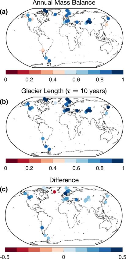
A. Huston et al.: Last millennium glacier variability 1649
√
stage models, which is set to 1/ 3; τ is the glacier response Comparing the columns of Fig. 2, we see the time se-
timescale; and β is a non-dimensional shape parameter that ries of L0 become increasingly smooth as τ increases. Dur-
only affects the amplitude of L0 and not its temporal charac- ing the pre-industrial period, positive trends in L0 across the
teristics. The glacier response time is given by Northern Hemisphere reflect a cooling trend within the LME
(i.e., Fig. 1b). Conversely, during the past century of anthro-
τ = −H /bt , (8) pogenic warming, negative trends in L0 are found at all loca-
tions for τ = 10 years but only in the Southern Hemisphere
where H is a characteristic ice thickness in the terminus for τ = 100 years. The lack of 20th-century retreat in the
zone and bt is the net (negative) mass balance in the termi- Northern Hemisphere partially reflects the muted warming
nus zone (Jóhannesson et al., 1989). Note there is not neces- trend in the LME relative to observations (Fig. A1). How-
sarily a simple relationship between τ and glacier size (e.g., ever, the difference in recent trends between τ = 10 and
Raper and Braithwaite, 2009; Bach et al., 2018). For exam- τ = 30 years also illustrates a more general point: namely,
ple, cirque glaciers can be thick and have termini that extend that higher τ values imply a more delayed response to a given
only a little past the equilibrium line altitude, giving them climate perturbation. We discuss the implications of this re-
τ ’s of many decades (e.g., Barth et al., 2018). Conversely, sult for future changes in glacier length in Sect. 4.
glaciers sourced from large accumulation areas may have ter- In addition to the ensemble-mean forced response, the
mini well below the equilibrium line altitude and, if terminat- panels in Fig. 2 also show glaciers exhibit significant differ-
ing on steep slopes, also be relatively thin, giving them short ences in ensemble spread. These differences are most clearly
τ ’s of a decade or less (e.g., Franz Joseph N.Z., Purdie et al., illustrated by the SNR values, which reveal two key depen-
2014). dencies. First, at all locations, SNR increases monotonically
The three-stage model accurately emulates the autocorre- with increasing τ (i.e., from left to right in Fig. 2). This im-
lation function and power spectrum of numerical flowline plies that large-τ glaciers are usually more reliable indica-
models of ice dynamics (Christian et al., 2018; Roe and tors of forced climate change than small-τ glaciers, which
Baker, 2014) and has been shown to produce realistic length are more prone to natural fluctuations. In the Appendix, we
responses to climate trends and variability given appropriate show that SNR also increases with τ at other locations as
choices of τ and β (e.g., Herla et al., 2017). well (Fig. A2), suggesting that it is a general property of the
In the simulations we present here, we did not attempt to climate system. There is a trade-off, however: the larger-τ
assign realistic values of τ and β to each glacier. Rather, for glaciers smooth over longer periods, and so the temporal res-
each glacier, we performed three separate simulations with olution of the forced change is degraded.
τ = 10, 30, and 100 years, and β = 150. This approach has Second, SNR is substantially greater in the spatially aver-
two main advantages. First, the subset of glaciers analyzed aged time series of glacier length (Fig. 2, bottom row) than
in Fig. 1 are located in regions with a wide range of glacier it is for any individual glacier, similar to what we found with
sizes. Simulating a range of response timescales thus gives a annual mass balance (Fig. 1). This suggests that glacier vari-
more complete picture of glacier variability in these regions. ability is more likely to reflect external forcing if it is coher-
Second, it allows us to perform a controlled test of how SNR ent across a large spatial domain.
varies with response timescale, which we will demonstrate We address each of these behaviors in the next section,
has important implications for how geologic records of past in which we also extend our analysis to the larger set of 76
glacier variability ought to be best interpreted. This range of glaciers, for which variability in summer and winter mass
τ encompasses most alpine glaciers (e.g., Haeberli and Hoel- balance was also provided by Medwedeff and Roe (2017, Ta-
zle, 1995; Lüthi and Bauder, 2010; Roe et al., 2017). The ble A1).
value of β is a function of glacier geometry: β = A/wH ,
where A is the surface area, and w and H are the characteris- 3.1 Dependence of signal-to-noise ratio on glacier
tic width and thickness of the glacier in the terminus zone. response time
Our choice of β = 150 is based on Hintereisferner in the
Austrian Alps (A = 10 km2 , w = 400 m, H = 170 m, Herla The dependence of SNR on τ can be understood by consid-
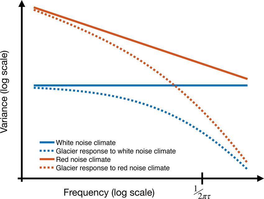
et al., 2017). The equation for L0 is linear, and so the value ering the spectra of climate variability and glacier length,
of β does not affect the relative importance of different kinds which are illustrated schematically in Fig. 3. The spectrum
of climate forcing. of a time series characterizes the variance as a function of
Figure 2 shows the glacier-length anomalies (L0 ) that re- frequency (e.g., Yiou et al., 1996). A climate with no inter-
sult from the time series of b0 (Fig. 1c) and for each of the annual persistence (i.e., no memory) is one that has no de-
three τ ’s considered. In each panel, the heavy line represents pendence on previous years, such that each year’s tempera-
the ensemble mean, while the light colors represent each of ture and precipitation are drawn independently from random
the 13 ensemble members. Note that the magnitude of the probability distributions. Such a climate is characterized by
length fluctuations is somewhat arbitrary and will change a white spectrum – one that has equal variance at all fre-
with catchment geometry. quencies (Fig. 3, solid blue line). A climate that has persis-
https://doi.org/10.5194/tc-15-1645-2021 The Cryosphere, 15, 1645–1662, 2021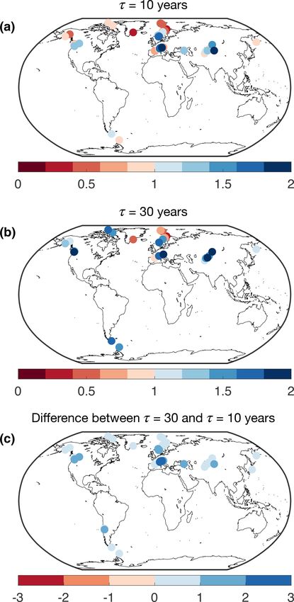
1650                                                                          A. Huston et al.: Last millennium glacier variability

Figure 2. Simulated glacier-length anomalies for representative glaciers in the Alps (top row), the Pacific Northwest (second row), and the
Patagonian Andes (third row). The fourth row shows the sum of all three glaciers. Each column shows results for different glacier response
times: τ = 10 years (left), τ = 30 years (middle), and τ = 100 years (right). Heavy colors represent the ensemble mean, while lighter colors
represent individual ensemble members. The vertical gray line at the year 1880 approximately marks the transition from the pre-industrial
era to the modern era. SNR values are computed over the pre-industrial era only. Bold font indicates SNR > 1, meaning that the forced signal
exceeds the noise of internal variability.

tence exhibits a red spectrum, with more variance at low fre-           spectrum of glacier length is generally redder than the unfil-
quencies (Fig. 3, solid red line). Different climate variables          tered spectra of temperature and precipitation (Fig. 3 dashed
can exhibit different degrees of persistence, with temperature          lines; Roe and Baker, 2014).
typically showing more persistence (and thus a redder spec-                The spectra of natural and forced variability are shown in
trum) than precipitation. Glacier dynamics then act as a low-           Fig. 4 and can be used to understand the variation of SNR
pass filter of this climate variability, causing the variance of        with τ (Fig. 2). They were calculated for the pre-industrial
glacier-length fluctuations to drop off sharply at frequencies          period (1000 to 1880). The rows in Fig. 4 show spectra for
higher than the cut-off frequency of (2π τ )−1 . As a result, the       annual mass balance (b), winter precipitation (P ), and sum-

The Cryosphere, 15, 1645–1662, 2021                                                          https://doi.org/10.5194/tc-15-1645-2021
A. Huston et al.: Last millennium glacier variability                                                                               1651

                                                                         (Fig. 4f). These are much more strongly red, with an average
                                                                         slope of −0.61, and are thus clearly responsible for the sim-
                                                                         ilarly reddened spectra of the forced mass balance (Fig. 4b).
                                                                         While there are some variations among the 76 glacier loca-
                                                                         tions (gray lines in Fig. 4), the broad features of these spectra
                                                                         are seen throughout our network.
                                                                            Interestingly, the redness of the forced mass-balance spec-
                                                                         tra in Fig. 4 is not evident in the spectrum of volcanic forcing,
                                                                         which is white at sub-decadal frequencies (Fig. A3). It must
                                                                         therefore be caused by reddening mechanisms inherent to the
                                                                         climate system, such as ocean heat storage and sea-ice feed-
                                                                         backs (Stenchikov et al., 2009; Miller et al., 2012). GCM
                                                                         simulations have further shown that strong, abrupt forcing
                                                                         from volcanic aerosols can also be reddened by enhanced
                                                                         heat exchange with the deep ocean, due to a strengthening
                                                                         of both vertical mixing and the Atlantic Meridional Over-
Figure 3. Schematic illustration of time series power spectra, rep-      turning Circulation (AMOC) (Stenchikov et al., 2009). This
resenting the relative magnitude of variance as a function of fre-       unique response to volcanic forcing may help explain why
quency. A white spectrum is flat (solid blue line), indicating uniform
                                                                         the forced spectra of T and b are so much redder than the un-
variance at all frequencies. A red spectrum has a negative slope
                                                                         forced spectra (Fig. 4). However, further research is needed
(solid red line), indicating greater variance at low frequencies. A
glacier acts as a low-pass filter, resulting in a redder spectrum for    to fully understand the difference in spectral slopes between
glacier length than for annual mass balance, which varies with tem-      forced and internal temperature variability.
perature and precipitation. The variance in annual mass balance that
is retained in time series of glacier length drops sharply beyond the    3.2   Dependence of signal-to-noise ratio on spatial scale
cut-off frequency of (2πτ )−1 .
                                                                         We now evaluate the spatial coherence of the forced
                                                                         and unforced responses among the set of 76 glaciers.
mer temperature (T ). Gray lines represent the spectra at the            Our 76 glaciers are clustered into a handful of specific
locations of all 76 glaciers in our data set; the colored lines          glacierized regions, which allows us to evaluate coherence
represent the subset of three glaciers analyzed in Figs. 1 and           within, and among, such regions. To facilitate compari-
2; and finally, the black line represents the average of all in-         son, we fix τ = 10 years and calculate the length fluctua-
dividual spectra across the 76 glaciers. Average slopes of the           tions using Eq. (7) at each of the 76 locations for (i) full
various spectra were calculated using linear regression and              mass balance, (ii) temperature-dependent mass balance, and
are shown in the bottom left of each panel.                              (iii) precipitation-dependent mass balance. Taking each of
   Comparing the spectra of unforced and forced mass-                    these three cases in turn, we calculate the correlation coef-
balance variability in the top row of Fig. 4, we find that the           ficient of the length history of each glacier with that of every
unforced spectrum is essentially white (i.e., a flat spectral            other glacier for the pre-industrial era (1000 to 1880). We
slope), while the forced spectrum is red (i.e., greater variance         present the results in matrix form in Fig. 5, for cases: (i) top
at low frequencies). Therefore, when low-pass-filtered by the            row, (ii) middle row, and (iii) bottom row. Although we show
glacier response, more of the forced variability is retained by          only the τ = 10 years, results for τ = 30 and 100 years were
the glacier, resulting in higher SNR values in glacier length            similar.
relative to annual mass balance. This effect becomes larger                 For natural variability (Fig. 5a), we find strong correla-
as τ increases and the filter cutoff shifts to lower frequen-            tions at the scale of individual glacierized regions but not at
cies, thus explaining the positive correlation between SNR               larger scales. For example, while all glaciers in the Alps are
and τ found in Fig. 2.                                                   strongly correlated with each other, they are not significantly
   The reason for the different slopes in the mass-balance               correlated with glaciers in Scandinavia. This implies that in-
spectra is due to differences in summer temperature. First,              ternal variability has a relatively short decorrelation length
consider the precipitation spectra for both forced and un-               scale, consistent with synoptic-scale atmospheric variability
forced variability (Fig. 4c–d). They are essentially flat at             (e.g., Wallace and Hobbs, 2006). When precipitation vari-
all frequencies, consistent with white noise of internal at-             ability alone is considered (Fig. 5c), we see anticorrelations
mospheric variability. Now consider the temperature spectra              between the Alps and Scandinavia, as well as within the set
of the unforced variability (Fig. 4e). It is only weakly red,            of Pacific Northwest glaciers. These anticorrelations reflect
with an average slope of −0.17; this slope equates to the ex-            dipoles in the patterns of interannual variability due to lati-
ponent α in a spectral power law of the form P ∝ f α . Fi-               tudinal shifts in the storm tracks associated with the North
nally, consider the temperature spectra for forced variability           Atlantic Oscillation and the Pacific North American patterns

https://doi.org/10.5194/tc-15-1645-2021                                                        The Cryosphere, 15, 1645–1662, 2021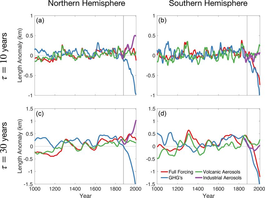
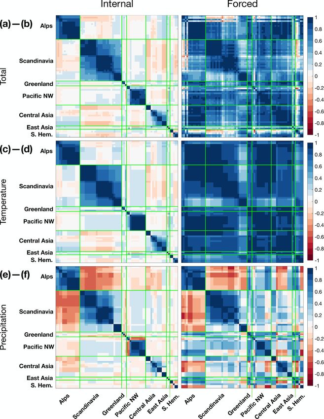
1652                                                                           A. Huston et al.: Last millennium glacier variability

Figure 4. Power spectra of forced and unforced variability for the pre-industrial era (1000 to 1880). Internal (unforced) variability is shown
in the left column (a, c, e) and forced variability in the right column (b, d, f). Top row (a, b) is annual mass balance, middle row (c, d) is
winter precipitation, and bottom row (e, f) is summer temperature. Spectra are shown for Silvretta (blue), South Cascade (red), Martial Este
(yellow), and the other 73 glaciers (gray). The black line shows the average of all 76 individual spectra. Lines in the bottom left of each
panel show the slope of the least-squares regression line for each spectrum. Spectra were computed using periodograms with a Hanning
window equal to one-third the length of the data. Unforced spectra were averaged among the 13 ensemble members. Forced spectra were
band-averaged to reduce noise, explaining the coarser spectral resolution.

and have been documented previously for glacier mass bal-                length are averaged across different mountain ranges, the in-
ance (e.g., Bitz and Battisti, 1999; Bonan et al., 2019). Such           coherent internal noise is damped relative to the coherent
anticorrelations are not generally strong enough to dominate             forced signal. This explains why the SNR of the averaged
the coherence of the overall length variability (Fig. 5a).               time series of glacier length is greater than the SNR at any
   For forced climate variability, cross correlations among              individual glacier (Fig. 2). Meanwhile, the decomposition of
glacier length are significantly positive among a large ma-              the forced correlations (Fig. 4d, f) shows that the global co-
jority of glacier pairs (92 %; Fig. 5b), indicating that climate         herence of forced glacier variability comes overwhelmingly
changes resulting from external forcing are globally coher-              from T rather than P . Precipitation-driven variability is a
ent (Fig. 5b). Moreover, when multiple time series of glacier

The Cryosphere, 15, 1645–1662, 2021                                                            https://doi.org/10.5194/tc-15-1645-2021
A. Huston et al.: Last millennium glacier variability                                                                                  1653

Figure 5. Matrix of cross correlations among the network of 76 glacier locations (Table A1), grouped by region. Each column or row in
the matrix shows the correlation coefficients of glacier length at one location with glacier length at every other location in the network,
calculated for the pre-industrial era (1000 to 1880). Left panels show results for internal variability, and the right panels shows results
for forced variability. Top row shows the results for the full mass-balance variability, while the middle and bottom rows show results for,
respectively, the temperature-only and precipitation-only components of the mass balance. Blue colors indicate positive correlations, and red
colors indicate negative correlations. A response time of τ = 10 years was used for these calculations.

source of noise that mostly weakens the correlations but does            vides little insight into the relative importance of tempera-
not change their global coherence.                                       ture versus precipitation in driving glacier variability more
                                                                         generally. These contributions are quantified in Fig. 6, which
3.3   The relative importance of precipitation versus                    shows the ratio of T -driven variance to total variance, both in
      temperature for mass balance and length                            annual mass balance (Fig. 6a) and in glacier length (Fig. 6b,
      fluctuations                                                       assuming τ = 10 years). Because variability in T and P is
                                                                         not significantly correlated at any glacier location, this ratio
The preceding analysis has shown that forced changes in                  approximately represents the fraction of total variance that
glacier length are driven primarily by globally coherent
changes in summer temperature. However, this result pro-

https://doi.org/10.5194/tc-15-1645-2021                                                         The Cryosphere, 15, 1645–1662, 2021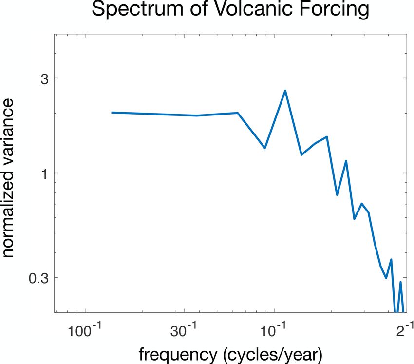
1654                                                                           A. Huston et al.: Last millennium glacier variability

                                                                         cific Northwest, and the Andes (Fig. 6a). In contrast, vari-
                                                                         ability in glacier length is dominated by temperature every-
                                                                         where (Fig. 6b), including at glaciers (like South Cascade)
                                                                         where precipitation accounts for most of the variability in
                                                                         annual mass balance. Averaged across all glaciers, tempera-
                                                                         ture accounts for 67 % of the total variance in annual mass
                                                                         balance and 83 % of the total variance in glacier length when
                                                                         τ = 10 years. Temperature’s share of the variance continues
                                                                         to increase with increasing τ but more modestly (to 86 %
                                                                         when τ = 30 years and 89 % when τ = 100 years).
                                                                            Why does temperature variability exert a greater influence
                                                                         on glacier length than on annual mass balance? Recall from
                                                                         Fig. 4 that the spectrum of T is redder than the spectrum
                                                                         of P . This difference is especially pronounced in the forced
                                                                         time series, but it is also evident in the unforced time series.
                                                                         Glaciers filter out variance at the highest frequencies, where
                                                                         precipitation’s contribution to annual-mass-balance variance
                                                                         is greatest. Thus, for the same reasons that SNR is enhanced
                                                                         by a glacier’s filtering properties, the contribution of tem-
                                                                         perature to glacier-length variability is enhanced relative to
                                                                         that of precipitation. This means that variability in glacier
                                                                         length primarily reflects low-frequency variability in summer
                                                                         temperature, even where mass-balance variability is more
                                                                         strongly influenced by winter precipitation.

                                                                         3.4   Roles of individual forcings

                                                                         Finally, we evaluate the relative importance of the different
                                                                         climate-forcing factors in these simulations. In addition to
                                                                         the full 13-member ensemble, the LME archive also contains
                                                                         smaller ensembles of simulations representing the climate re-
                                                                         sponse to single factors. The factors (and the number of en-
                                                                         semble members) are greenhouse gases (3), volcanic aerosols
                                                                         (5), industrial aerosols (5), and changes in solar and orbital
                                                                         patterns (3). As in the full-forcing ensemble, we use the en-
                                                                         semble mean to approximate the climate response to each
                                                                         individual factor. However, it is important to note that these
Figure 6. The importance of summertime temperature in driv-              approximations contain substantially more noise than the full
ing overall variance in mass balance and glacier length across the
                                                                         ensemble mean because there are fewer ensemble members.
glacier network, calculated for the pre-industrial era (1000 to 1880).
Panel (a) shows the fraction of total variance in mass balance that is
                                                                            Figure 7 shows the time series of glacier-length anomalies
due to summer temperature. Panel (b) shows the same thing, but for       induced by each individual forcing factor, averaged among
glacier length. The difference is shown in panel (c), from which we      all ensemble members and all glaciers in the Northern Hemi-
see that, in all but one case (Mittivakkat in Greenland), summer tem-    sphere (left) and Southern Hemisphere (right). Results are
perature accounts for a larger fraction of variance in glacier length    presented for τ = 10 years (top) and τ = 30 years (bottom).
than in annual mass balance. This is due to the low-pass-filtering       The contributions from the solar and orbital forcing were
properties of glacier dynamics.                                          negligible and are not shown.
                                                                            During the pre-industrial era, most of the forced variabil-
                                                                         ity in glacier length can be attributed to volcanic aerosols, as
can be attributed to T . The difference between the two pan-             indicated by the similar behavior of the red and green lines
els is shown in Fig. 6c.                                                 in Fig. 7. Over the last century, however, anthropogenic fac-
   In the case of annual mass balance (Fig. 6a), T accounts              tors have played the largest role. In the Southern Hemisphere,
for more than half the variance at 58 out of 76 glaciers. The            the full-forcing time series closely follows greenhouse-gas-
relatively few glaciers where precipitation variability plays            driven trends beginning around the year 1850. In the North-
a larger role are mostly located in maritime environments                ern Hemisphere, by contrast, retreat due to greenhouse gases
with large storm-track variability, such as Alaska, the Pa-              is largely offset by industrial aerosol emissions during the

The Cryosphere, 15, 1645–1662, 2021                                                         https://doi.org/10.5194/tc-15-1645-2021
A. Huston et al.: Last millennium glacier variability 1655
Figure 7. Contributions of individual forcing factors to glacier-length variability over the last millennium. Results are shown for response
timescales of τ = 10 years (a, b) and τ = 30 years (c, d). The left column (a, c) shows the average of all Northern Hemisphere glaciers in
our network, and the right column (b, d) shows the average of all Southern Hemisphere glaciers. Colors represent the contributions from
individual forcing factors, which we approximate from the ensemble-mean time series of summer temperature and winter precipitation within
each single-forcing ensemble. The individual forcing factors are greenhouses gases (blue), volcanic aerosols (green), and industrial aerosols
(purple). The red line shows the combined influence of all forcing factors diagnosed from the full 13-member ensemble.The gray vertical
line marks the transition from the pre-industrial to modern eras at year 1880.
modern era. While it is well known that industrial aerosols and winter precipitation from the 13-member CESM Last
provided radiative cooling over the 20th century, warming Millennium Ensemble. Using the three-stage linear model
trends over this period are generally lower in the LME than of Roe and Baker (2014), we then converted these mass-
in observations (Fig. A1), suggesting that the model’s aerosol balance anomalies into glacier-length anomalies for a range
forcing may be too strong or that its transient climate sen- of glacier response timescales, thus capturing the diversity
sitivity may be too low. Whatever the cause, the suppressed of behavior exhibited by glaciers of different sizes and ge-
20th-century warming trend in many regions within the LME ometries. Because the ensemble simulations differ only in
explains why, in some locations, our simulations appear to their initial conditions, the responses of mass balance and
show less glacier retreat than has been observed. glacier length to external radiative forcing are mostly cap-
tured by the ensemble mean, while internal unforced vari-
ability is represented by departures from the ensemble mean
(i.e., the ensemble spread). The ratio of ensemble-mean vari-
4 Summary and discussion
ance to ensemble-spread variance is defined as the signal-to-
In this study, we have combined an ensemble of numeri- noise ratio (SNR) and represents the fraction of total variance
cal climate model simulations and a glacier length model driven by external forcing.
to evaluate the relative importance of climate forcing and While SNR varies by location, we found that two fac-
internal climate variability in driving glacier-length fluctu- tors influence SNR more generally. First, SNR is greater for
ations over the last millennium. While the potential impor- glacier length than for annual mass balance and continues in-
tance of internal variability has been noted before, this is the creasing with increasing glacier response timescale, τ . This
first study to evaluate the relative importance of natural forc- timescale dependence reflects differences in how forced and
ing vs. internal variability in the pre-industrial era and the unforced mass-balance variance is distributed across the fre-
accompanying spatial patterns of glacier response. We esti- quency spectrum. Specifically, because forced variance has a
mated annual-mass-balance anomalies at 76 glaciers around redder spectrum than unforced variance, the forced signal is
the world using simulated time series of summer temperature amplified relative to unforced noise when low-pass-filtered
https://doi.org/10.5194/tc-15-1645-2021 The Cryosphere, 15, 1645–1662, 20211656 A. Huston et al.: Last millennium glacier variability by a glacier. This explains why a glacier like South Cas- Finally, we have analyzed time series of glacier-length cade, which does not exhibit a significant forced response fluctuations. Of course, in actuality glacial history is recorded in annual mass balance due to high interannual variability mostly by the dating of moraines on the landscape. Moraines (Fig. 1, red), nonetheless shows a significant forced response are created by many different physical processes (e.g., An- in glacier length in our simulations (Fig. 2, red). derson et al., 2014, for a review of processes and formation Second, for both mass balance and glacier length, SNR is times), and dating resolution and accuracy limit the ability enhanced by averaging multiple length histories from differ- to evaluate the coherence of glacier advances in different re- ent locations. This is because forced changes in mass balance gions (Schaefer et al., 2009; Balco, 2009). Moreover, differ- tend to be globally coherent, reflecting a global-scale tem- ent glacier response times affect the phase relationship be- perature response, while unforced variability has little coher- tween the timing of a cooling and the response of glacier ence beyond the scale of one glacierized region. Our analyses length. So a careful assessment of glacier dynamics should suggest that forced changes in glacier length are driven pri- be incorporated into any comparison of moraine histories marily by globally coherent changes in summer temperature from different locations, as done, for example, in Young et al. and that, in the pre-industrial era, those arise from volcanic- (2011). A natural extension of the present work would be aerosol forcing. to incorporate a simple moraine model (e.g., Gibbons et al., Our results have implications for how past glacier vari- 1984; Anderson et al., 2014) and to evaluate the spatial co- ability should be interpreted. For example, because SNR in- herence of moraine statistics. creases with spatial averaging, a change in glacier length is Our analyses have been made possible by ensemble cli- more likely to be forced when coherent changes are also ob- mate modeling. As done here, such ensembles can be used to served in other regions. decompose the contributions due to internal variability and However, it is important to recognize that the amplified natural and anthropogenic forcing. However, we have used signal in large-τ glaciers comes at the expense of decreased only one climate model. As other ensembles become more temporal resolution. Thus, while large-τ glaciers may be widely available it will be important to evaluate different cli- more reliable indicators of climate change on centennial mate models, and also different estimates of the natural and timescales, they may entirely miss climate changes that occur anthropogenic forcing, for which there are still significant on multi-decadal timescales. uncertainties (Schmidt et al., 2011). Differences in response time also have implications for how glaciers have responded and will respond to global warming. Because glaciers are lagging indicators of climate change, recent glacier retreat has been more modest than the decrease in annual mass balance (Figs. 1 and 2), implying that further retreat is locked in, even in the absence of addi- tional warming (Christian et al., 2018). This disequilibrium is especially pronounced for large-τ glaciers, whose slow re- sponse means that they have only begun to feel the effects of the past century of warming. In future decades, therefore, we expect that large-τ glaciers will experience the greatest retreat, as they integrate the effects of both past and future warming. The Cryosphere, 15, 1645–1662, 2021 https://doi.org/10.5194/tc-15-1645-2021
A. Huston et al.: Last millennium glacier variability                                                                         1657

Appendix A: Statistical significance of SNR

We consider a signal-to-noise ratio (SNR) to be statistically
significant if we can reject the null hypothesis that SNR = 0
with at least 99 % confidence (p < 0.01). To determine the
threshold for statistical significance, we performed a Monte
Carlo simulation consisting of 100 000 ensembles of 13 ran-
domly generated Gaussian time series (i.e., noise). We set
the length of each synthetic time series based on the esti-
mated degrees of freedom in the given climate variable, as
described below. For each 13-member ensemble, we com-
pute the SNR as in Eq. (6). This yields a set of 100 000 syn-
thetic SNR values which have a mean of 0.083 and a distri-
bution that depends on the number of degrees of freedom in
the time series. Because the true SNR of each ensemble is
equal to 0, we set the threshold for statistical significance to
be the 99th percentile of SNR values within the distribution.
   At all glacier locations within the LME, we find that time
series of winter precipitation and summer temperature ex-
hibit an e-folding decorrelation scale of no more than 1 year.
Thus, for time series of summer and winter mass balance, we
assume the number of degrees of freedom is equal to half the
number of years in the stated time period (Leith, 1973). This
yields significance thresholds of 0.098 for the pre-industrial
era and 0.125 for the modern era.
   For the glacier-length time series, we find that the e-
folding decorrelation scale is on average equal to about 1.5τ .
Over the pre-industrial period, this implies about 30, 10, and
3 degrees of freedom for τ = 10, 30, and 100 years, respec-
tively. The corresponding SNR significance thresholds are
found to be 0.15 for τ = 10 years, 0.22 for τ = 30 years, and
0.49 for τ = 100 years. All of our simulated glacier-length
time series have SNR values that exceed these thresholds.

                                                                   Figure A1. Linear trend in 2 m air temperature (in units of
                                                                   K/century) between 1900–1999 in (a) the NASA GISS observa-
                                                                   tional dataset and (b) the CESM LME ensemble mean. (c) The dif-
                                                                   ference between panels (a) and (b). Warmer temperatures are shown
                                                                   in red, with cooler temperatures shown in blue.

https://doi.org/10.5194/tc-15-1645-2021                                                  The Cryosphere, 15, 1645–1662, 2021
1658 A. Huston et al.: Last millennium glacier variability
Figure A3. Power spectrum of volcanic forcing generated from
time series of volcanic aerosol concentrations in the LME (courtesy
of John Fasullo).
Figure A2. The signal-to-noise ratio (SNR) of glacier length for all
76 glacier locations given (a) τ = 10 years and (b) τ = 30 years.
(c) The difference between panels (b) and (a). Red colors in pan-
els (a) and (b) indicate a larger role for internal variability than
forced variability, while blue colors indicate the opposite. Blue col-
ors in panel (c) indicate a greater role for forced variability when
τ = 30 years than when τ = 10 years.
The Cryosphere, 15, 1645–1662, 2021 https://doi.org/10.5194/tc-15-1645-2021A. Huston et al.: Last millennium glacier variability 1659
Table A1. Glacier data from Medwedeff and Roe (2017), sorted by region. Glaciers are excluded if observations of summer or winter mass
balance span less than 10 years. σb,w : the standard deviation of observed winter mass balance (in m). σb,s : the standard deviation of observed
summer mass balance (in m). σP : the standard deviation of simulated winter precipitation within the LME over the last millennium (1000–
1999) (in m). σT : the standard deviation of simulated summer temperature within the LME over the last millennium (1000–1999) (in K). α:
the ratio of σb,w /σP . λ: the ratio of σb,s /σT (in m/K).
Glacier/region Lat Long σb,w σb,s σP σT α λ
Alps/Pyrenees
Ossoue 42.77 −0.14 0.54 0.78 0.07 0.69 7.49 1.14
Maladeta 42.65 0.63 0.51 0.64 0.06 0.81 7.99 0.79
Sarennes 45.13 6.13 0.51 0.85 0.07 0.72 7.03 1.17
Grand Etret 45.47 7.21 0.58 0.47 0.09 0.76 6.55 0.61
Gries 46.44 8.33 0.39 0.63 0.09 0.60 4.20 1.04
Ciardoney 45.51 7.39 0.49 1.29 0.09 0.60 5.25 2.15
Basodino 46.42 8.48 0.48 0.62 0.09 0.60 5.19 1.03
Silvretta 46.85 10.08 0.34 0.67 0.09 0.60 3.86 1.11
Vernagtferner 46.88 10.82 0.22 0.42 0.09 0.60 2.52 0.70
Fontana Bianca/Weissbrunnferner 46.48 10.77 0.38 0.61 0.09 0.60 4.30 1.01
Jamtalferner 46.87 10.17 0.25 0.49 0.09 0.60 2.88 0.81
Careser 46.45 10.70 0.38 0.44 0.09 0.60 4.28 0.74
Wurtenkees 47.03 13.00 0.29 0.57 0.09 0.64 3.24 0.89
Kleinfleisskees 47.05 12.95 0.26 0.54 0.09 0.64 2.90 0.85
Goldbergkees 47.04 12.97 0.25 0.56 0.09 0.64 2.72 0.88
Scandinavia
Rembesdalskaaka 60.53 7.36 0.75 0.54 0.14 0.71 5.27 0.76
Graafjellsbrea 60.08 6.39 0.73 0.60 0.14 0.71 5.12 0.84
Breidablikkbrea 60.07 6.36 0.80 0.55 0.14 0.71 5.58 0.78
Aalfotbreen 61.75 5.65 1.07 0.73 0.19 0.67 5.76 1.08
Hansbreen 77.08 15.67 0.17 0.29 0.07 1.70 2.33 0.17
Storbreen 61.57 8.13 0.38 0.47 0.16 0.84 2.39 0.56
Hellstugubreen 61.56 8.44 0.27 0.50 0.16 0.84 1.73 0.60
Nigardsbreen 61.72 7.13 0.61 0.59 0.16 0.84 3.88 0.70
Graasubreen 61.65 8.60 0.25 0.51 0.16 0.84 1.56 0.60
Austdalsbreen 61.81 7.35 0.65 0.62 0.16 0.84 4.10 0.74
Okstindbreen 66.01 14.29 0.69 0.51 0.08 1.01 8.75 0.50
Engabreen 66.65 13.85 0.78 0.71 0.12 1.00 6.21 0.70
Storglombreen 66.67 14.00 0.50 0.72 0.12 1.00 3.97 0.72
Trollbergdalsbreen 66.71 14.44 0.53 0.57 0.12 1.00 4.21 0.57
Storglaciaeren 67.90 18.57 0.38 0.49 0.06 1.08 6.00 0.45
Riukojietna 68.08 18.08 0.39 0.59 0.06 1.08 6.17 0.54
Rabots 67.91 18.50 0.38 0.47 0.06 1.08 6.13 0.44
Tarfalaglaciaeren 67.93 18.65 0.44 0.74 0.06 1.08 7.01 0.68
Marmaglaciaeren 68.83 18.67 0.21 0.46 0.09 1.03 2.36 0.44
Storsteinsfjellbreen 68.22 17.92 0.35 0.29 0.09 1.03 3.96 0.28
Langfjordjoekulen 70.12 21.73 0.36 0.52 0.06 1.11 5.70 0.47
Austre Broeggerbreen 78.88 11.83 0.12 0.30 0.05 1.48 2.36 0.20
Midtre Lovénbreen 78.88 12.07 0.13 0.29 0.05 1.48 2.65 0.20
Kongsvegen 78.80 12.98 0.15 0.31 0.05 1.48 3.03 0.21
Waldemarbreen 78.67 12.00 0.13 0.17 0.05 1.48 2.66 0.11
Greenland/NE Canada
Meighen Ice Cap 79.95 −99.13 0.03 0.28 0.02 1.13 1.93 0.25
Devon Ice Cap NW 75.42 −83.25 0.02 0.16 0.02 1.32 1.30 0.12
Mittivakkat 65.67 −37.83 0.14 0.37 0.21 1.27 0.69 0.29
https://doi.org/10.5194/tc-15-1645-2021 The Cryosphere, 15, 1645–1662, 20211660 A. Huston et al.: Last millennium glacier variability
Table A1. Continued.
Glacier/region Lat Long σb,w σb,s σP σT α λ
Alaska/PNW
Gulkana 63.25 −145.42 0.29 0.51 0.05 1.06 6.52 0.48
Wolverine 60.40 −148.92 0.80 0.65 0.12 1.04 6.91 0.63
Peyto 51.67 −116.53 0.40 0.38 0.05 0.73 7.83 0.53
Place 50.43 −122.60 0.31 0.47 0.19 0.88 1.60 0.54
Sentinel 49.90 −122.98 0.67 0.47 0.19 0.88 3.43 0.54
Helm 49.97 −123.00 0.41 0.56 0.19 0.88 2.11 0.64
Zavisha 50.80 −123.42 0.31 0.51 0.19 0.88 1.60 0.58
Sykora 50.87 −123.58 0.27 0.54 0.19 0.88 1.40 0.62
Silver 48.98 −121.25 0.72 0.98 0.19 0.68 3.80 1.44
Noisy Creek 48.67 −121.53 0.99 1.13 0.19 0.68 5.22 1.66
South Cascade 48.37 −121.05 0.65 0.58 0.16 0.68 4.18 0.85
North Klawatti 48.57 −121.12 0.91 1.15 0.16 0.68 5.83 1.69
Central Asia
Djankuat 43.20 42.77 0.41 0.46 0.07 0.74 5.93 0.62
Garabashi 43.30 42.47 0.17 0.41 0.07 0.74 2.48 0.56
Tbilisa 43.13 42.47 0.14 0.31 0.07 0.74 2.05 0.43
Abramov 39.63 71.6 0.32 0.41 0.08 0.93 4.02 0.44
Golubin 42.46 74.49 0.15 0.23 0.04 0.72 3.74 0.32
Tsentralniy Tuyuksuyskiy 43.05 77.08 0.21 0.44 0.03 0.65 7.94 0.68
Shumskiy 45.08 80.23 0.08 0.42 0.03 0.74 2.78 0.57
Urumqi Glacier No. 1 W-Branch 43.08 86.82 0.09 0.44 0.01 0.58 15.08 0.76
Urumqi Glacier No. 1 43.08 86.82 0.09 0.33 0.01 0.58 15.46 0.57
Urumqi Glacier No. 1 E-Branch 43.08 86.82 0.06 0.36 0.01 0.58 10.18 0.62
Maliy Aktru 50.08 87.75 0.27 0.30 0.05 0.69 5.76 0.43
Vodopadniy 50.10 87.70 0.10 0.22 0.05 0.69 2.09 0.32
Leviy Aktru 50.08 87.72 0.15 0.24 0.05 0.69 3.16 0.35
East Asia
Hamaguri Yuki 36.60 137.62 1.63 1.52 0.08 0.70 19.69 2.18
Kozelsky 53.23 158.82 0.61 1.22 0.09 1.05 6.84 1.16
Southern Hemisphere
Echaurren Norte −33.57 −70.13 1.24 0.71 0.13 0.63 9.71 1.12
Piloto Este −32.22 −70.05 0.58 0.55 0.13 0.63 4.58 0.87
Martial Este −54.78 −68.40 0.28 0.49 0.04 0.49 7.10 1.00
Johnsons −62.66 −60.35 0.17 0.22 0.05 0.99 3.38 0.22
Hurd −62.68 −60.40 0.14 0.30 0.05 0.99 2.72 0.31
The Cryosphere, 15, 1645–1662, 2021 https://doi.org/10.5194/tc-15-1645-2021A. Huston et al.: Last millennium glacier variability 1661
Data availability. Monthly output variables from the CESM Last Burke, E. E. and Roe, G. H.: The absence of memory in the
Millennium Ensemble can be downloaded from the National climatic forcing of glaciers, Clim. Dynam., 42, 1335–1346,
Center for Atmospheric Research (NCAR) Climate Data Gateway: https://doi.org/10.1007/s00382-013-1758-0, 2014.
https://www.earthsystemgrid.org/dataset/ucar.cgd.ccsm4.CESM_ Christian, J. E., Koutnik, M., and Roe, G.: Committed retreat: con-
CAM5_LME.atm.proc.monthly_ave.html (Otto-Bliesner et al., trols on glacier disequilibrium in a warming climate, J. Glaciol.,
2016). 64, 675–688, https://doi.org/10.1017/jog.2018.57, 2018.
Crowley, T. J.: Causes of climate change over
the past 1000 years, Science, 289, 270–277,
Author contributions. AH and NS performed the analysis and https://doi.org/10.1126/science.289.5477.270, 2000.
wrote the first draft. GHR and NS designed the study. All authors Deser, C., Phillips, A., Bourdette, V., and Teng, H.: Uncertainty
helped interpret the results and edit the paper. in climate change projections: The role of internal variabil-
ity, Clim. Dynam., 38, 527–546, https://doi.org/10.1007/s00382-
010-0977-x, 2012.
Competing interests. The authors declare that they have no conflict Gibbons, A. B., Megeath, J. D., and Pierce, K. L.: Proba-
of interest. bility of moraine survival in a succession of glacial ad-
vances., Geology, 12, 327–330, https://doi.org/10.1130/0091-
7613(1984)122.0.CO;2, 1984.
Guillet, S., Corona, C., Stoffel, M., Khodri, M., Lavigne, F., Ortega,
Acknowledgements. We thank John Fasullo for providing time se-
P., Eckert, N., Sielenou, P. D., Daux, V., Churakova Sidorova,
ries of individual forcing agents used in the LME. We thank the Ore-
O. V., Davi, N., Edouard, J. L., Zhang, Y., Luckman, B. H.,
gon State University Honors College for supporting this research.
Myglan, V. S., Guiot, J., Beniston, M., Masson-Delmotte, V.,
This is LDEO contribution number 8484.
and Oppenheimer, C.: Climate response to the Samalas volcanic
eruption in 1257 revealed by proxy records, Nat. Geosci., 10,
123–128, https://doi.org/10.1038/ngeo2875, 2017.
Financial support. This research has been supported by the Na- Haeberli, W. and Hoelzle, M.: Application of inventory data
tional Science Foundation, Directorate for Geosciences (grant nos. for estimating characteristics of and regional climate-
AGS-2024212, AGS-1805490, and AGS-1903465). change effects on mountain glaciers: a pilot study
with the European Alps, Ann. Glaciol., 21, 206–212,
https://doi.org/10.3189/s0260305500015834, 1995.
Review statement. This paper was edited by Valentina Radic and Harrison, W. D. and Post, A. S.: How much do we re-
reviewed by two anonymous referees. ally know about glacier surging?, Ann. Glaciol., 36, 1–6,
https://doi.org/10.3189/172756403781816185, 2003.
Haustein, K., Otto, F. E., Venema, V., Jacobs, P., Cowtan, K.,
Hausfather, Z., Way, R. G., White, B., Subramanian, A., and
Schurer, A. P.: A limited role for unforced internal variabil-
References ity in twentieth-century warming, J. Climate, 32, 4893–4917,
https://doi.org/10.1175/JCLI-D-18-0555.1, 2019.
Anderson, L. S., Roe, G. H., and Anderson, R. S.: The effects of Herla, F., Roe, G. H., and Marzeion, B.: Ensemble statistics of
interannual climate variability on the moraine record, Geology, a geometric glacier length model, Ann. Glaciol., 58, 130–135,
42, 55–58, https://doi.org/10.1130/G34791.1, 2014. https://doi.org/10.1017/aog.2017.15, 2017.
Bach, E., Radic, V., and Schoof, C.: How sensitive are moun- Jóhannesson, T., Raymond, C., and Waddington, E.: Time–Scale for
tain glaciers to climate change? Insights from a block model, Adjustment of Glaciers to Changes in Mass Balance, J. Glaciol.,
J. Glaciol., 64, 247–258, https://doi.org/10.1017/jog.2018.15, 35, 355–369, https://doi.org/10.3189/S002214300000928X,
2018. 1989.
Balco, G.: The Geographic Footprint of Glacier Change, Science, Leith, C.: The Standard Error of Time-Average Es-
324, 599–600, https://doi.org/10.1126/science.1172468, 2009. timates of Climatic Means, J. Appl. Meteorol.
Barth, A. M., Clark, P. U., Clark, J., Roe, G. H., Marcott, S. A., Clim., 12, 1066–1069, https://doi.org/10.1175/1520-
Marshall McCabe, A., Caffee, M. W., He, F., Cuzzone, J. K., 0450(1973)0122.0.CO;2, 1973.
and Dunlop, P.: Persistent millennial-scale glacier fluctuations Lenssen, N., Schmidt, G., Hansen, J., Menne, M., Persin, A.,
in Ireland between 24 ka and 10 ka, Geology, 46, 151–154, Ruedy, R., and Zyss, D.: Improvements in the GISTEMP un-
https://doi.org/10.1130/G39796.1, 2018. certainty model, J. Geophys. Res.- Atmos., 124, 6307–6326,
Bitz, C. M. and Battisti, D. S.: Interannual to decadal https://doi.org/10.1029/2018JD029522, 2019.
variability in climate and the glacier mass balance Lüthi, M. P. and Bauder, A.: Analysis of Alpine glacier length
in Washington, Western Canada, and Alaska, J. Cli- change records with a macroscopic glacier model, Geogr. Helv.,
mate, 12, 3181–3196, https://doi.org/10.1175/1520- 65, 92–102, https://doi.org/10.5194/gh-65-92-2010, 2010.
0442(1999)0122.0.CO;2, 1999. Medwedeff, W. G. and Roe, G. H.: Trends and variability in the
Bonan, D. B., Christian, J. E., and Christianson, K.: Influence global dataset of glacier mass balance, Clim. Dynam., 48, 3085–
of North Atlantic climate variability on glacier mass balance 3097, https://doi.org/10.1007/s00382-016-3253-x, 2017.
in Norway, Sweden and Svalbard, J. Glaciol., 65, 580–594,
https://doi.org/10.1017/jog.2019.35, 2019.
https://doi.org/10.5194/tc-15-1645-2021 The Cryosphere, 15, 1645–1662, 2021You can also read