WHAT WAS THE SOURCE OF THE ATMOSPHERIC CO2 INCREASE DURING THE HOLOCENE? - MPG.PURE
←
→
Page content transcription
If your browser does not render page correctly, please read the page content below
Biogeosciences, 16, 2543–2555, 2019
https://doi.org/10.5194/bg-16-2543-2019
© Author(s) 2019. This work is distributed under
the Creative Commons Attribution 4.0 License.

What was the source of the atmospheric CO2 increase
during the Holocene?
Victor Brovkin1 , Stephan Lorenz1 , Thomas Raddatz1 , Tatiana Ilyina1 , Irene Stemmler1 , Matthew Toohey2 , and
Martin Claussen1,3
1 Max-Planck Institute for Meteorology, Hamburg, Germany
2 GEOMAR    Helmholtz Centre for Ocean Research Kiel, Kiel, Germany
3 Meteorological Institute, University of Hamburg, Hamburg, Germany

Correspondence: Victor Brovkin (victor.brovkin@mpimet.mpg.de)

Received: 22 February 2019 – Discussion started: 4 March 2019
Revised: 7 June 2019 – Accepted: 12 June 2019 – Published: 2 July 2019

Abstract. The atmospheric CO2 concentration increased by            face alkalinity decrease, for example due to unaccounted for
about 20 ppm from 6000 BCE to the pre-industrial period             carbonate accumulation processes on shelves, is required for
(1850 CE). Several hypotheses have been proposed to ex-             consistency with ice-core CO2 data. Consequently, our sim-
plain mechanisms of this CO2 growth based on either ocean           ulations support the hypothesis that the ocean was a source
or land carbon sources. Here, we apply the Earth system             of CO2 until the late Holocene when anthropogenic CO2
model MPI-ESM-LR for two transient simulations of climate           sources started to affect atmospheric CO2 .
and carbon cycle dynamics during this period. In the first
simulation, atmospheric CO2 is prescribed following ice-
core CO2 data. In response to the growing atmospheric CO2
concentration, land carbon storage increases until 2000 BCE,        1   Introduction
stagnates afterwards, and decreases from 1 CE, while the
ocean continuously takes CO2 out of the atmosphere after            The recent interglacial period, the Holocene, began in
4000 BCE. This leads to a missing source of 166 Pg of carbon        about 9700 BCE (Before Common Era) and is character-
in the ocean–land–atmosphere system by the end of the simu-         ized by a relatively stable climate. In geological archives,
lation. In the second experiment, we applied a CO2 nudging          the Holocene is the best recorded period, making it pos-
technique using surface alkalinity forcing to follow the re-        sible to reconstruct changes in climate and vegetation in
constructed CO2 concentration while keeping the carbon cy-          remarkable detail (e.g. Wanner et al., 2008). Proxy-based
cle interactive. In that case the ocean is a source of CO2 from     reconstructions suggest a decrease in sea surface tempera-
6000 to 2000 BCE due to a decrease in the surface ocean al-         tures in the North Atlantic (Marcott et al., 2013; Kim et al.,
kalinity. In the prescribed CO2 simulation, surface alkalinity      2004) simultaneous with an increase in land temperature in
declines as well. However, it is not sufficient to turn the ocean   western Eurasia (Baker et al., 2017), so that net changes in
into a CO2 source. The carbonate ion concentration in the           the global temperature are small. From Antarctic ice-core
deep Atlantic decreases in both the prescribed and the inter-       records, we know that the atmospheric CO2 concentration
active CO2 simulations, while the magnitude of the decrease         increased by about 20 ppm between 5000 BCE and the pre-
in the prescribed CO2 experiment is underestimated in com-          industrial period (Monnin et al., 2004; Schmitt et al., 2012;
parison with available proxies. As the land serves as a carbon      Schneider et al., 2013). Hypotheses explaining CO2 growth
sink until 2000 BCE due to natural carbon cycle processes           in the Holocene could be roughly subdivided into ocean-
in both experiments, the missing source of carbon for land          and land-based. The ocean mechanisms include changes in
and atmosphere can only be attributed to the ocean. Within          carbonate chemistry as a result of carbonate compensation
our model framework, an additional mechanism, such as sur-          to deglaciation processes (Broecker et al., 1999, 2001; Joos
                                                                    et al., 2004), redistribution of carbonate sedimentation from

Published by Copernicus Publications on behalf of the European Geosciences Union.
2544 V. Brovkin et al.: What was the atmospheric CO2 source in the Holocene?
the deep ocean to shelves, mostly due to coral reef regrowth surface model JSBACH (Raddatz et al., 2007; Reick et al.,
(Ridgwell et al., 2003; Kleinen et al., 2016), CO2 degassing 2013), and the marine biogeochemistry model HAMOCC5
due to an increase in sea surface temperatures, predominantly (Ilyina et al., 2013). In comparison to the MPI-ESM-LR
in the tropics (Indermühle et al., 1999; Brovkin et al., 2008), model used in the Climate Model Intercomparison Project
and a decrease in the marine soft tissue pump in response to Phase 5 (CMIP5) simulations (Giorgetta et al., 2013), the
circulation changes (Goodwin et al., 2011). Using a deconvo- model has been updated with several new components for
lution approach based on ice-core CO2 and δ 13 C data, Elsig the land hydrology and carbon cycle. In addition to the pre-
et al. (2009) concluded that a significant fraction of Holocene viously developed dynamic vegetation model (Brovkin et al.,
CO2 changes were attributed to carbonate compensation ef- 2009), the new JSBACH component includes the soil car-
fects during deglaciation. Recent synthesis of carbon burial bon model YASSO (Goll et al., 2015), a five-layer hydrol-
in the ocean during the last glacial cycle suggests excessive ogy scheme (Hagemann and Stacke, 2015), and an interac-
accumulation of CaCO3 and organic carbon in the ocean sed- tive albedo scheme (Vamborg et al., 2011). HAMOCC was
iments during deglaciation and Holocene (Cartapanis et al., updated with prognostic nitrogen fixers (Paulsen et al., 2017)
2018), implicitly supporting the ocean-based mechanism of and a parameterization for a depth-dependent detritus settling
atmospheric CO2 growth in response to a decrease in the velocity and remineralization of organic material (Martin et
ocean alkalinity. al., 1987).
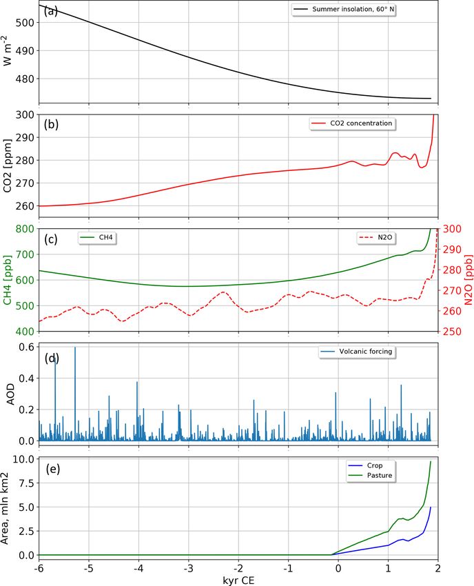
The land-based explanations suggest a reduction in natural We used a combination of several forcings as boundary
vegetation cover, such as decreased boreal forests’ area and conditions for transient simulations (Fig. 1). The orbital forc-
increased desert in North Africa (e.g. Foley, 1994; Brovkin ing (Fig. 1a) follows a reconstruction by Berger (1978). We
et al., 2002) and anthropogenic land cover changes, mainly use a solar irradiance forcing that was reconstructed from 14 C
deforestation (Ruddiman, 2003, 2017; Kaplan et al., 2011; tree-ring data that correlate with the past changes in the so-
Stocker et al., 2014, 2017). A couple of land processes (CO2 lar open magnetic field (Krivova et al., 2011). CO2 , N2 O,
fertilization, peat accumulation) should have led to terres- and CH4 forcings stem from ice-core reconstructions (Fortu-
trial carbon increase in the Holocene (Yu, 2012; Stocker et nat Joos, personal communication, 2016, Fig. 1b,c); see also
al., 2017), complicating the land source explanation. The comment by Köhler (2019). We applied a new reconstruc-
land-based hypotheses, as well as the ocean soft tissue pump tion of volcanic forcing (Bader et al., 2019) based on the
explanation, also have difficulty conforming with the at- GISP2 ice-core volcanic sulfate record (Zielinski et al., 1996)
mospheric δ 13 CO2 reconstructions that show no substan- (Fig. 1d). To maintain consistency with the CMIP5 simula-
tial changes in the Holocene (Schmitt et al., 2012; Schnei- tions, we included the land use changes based on the LUH1.0
der et al., 2013), contrary to the expectation of a signif- product by Hurrt et al. (2011) and Pongratz et al. (2011), pro-
icant atmospheric δ 13 CO2 decrease due to the release of vided for the period after 850 CE. To avoid an abrupt change
isotopically light biological carbon. The deconvolution ap- in the land use forcing at 850 CE, we interpolated the land
proach by Elsig et al. (2009) suggested a land carbon up- use map from 850 CE linearly backwards to no land use con-
take of 290 GtC between 9000 and 3000 BCE. For a de- ditions at 150 BCE (Fig. 1e). The land use areas in 1750 CE
tailed overview of process-based hypotheses, see, for exam- are in line with the most recent update of the HYDE dataset
ple, Brovkin et al. (2016). (Klein Goldewijk et al., 2017), although our interpolation un-
While many numerical experiments have been done to test derestimates crop and pasture areas earlier than 1750 CE.
the above-mentioned hypotheses with intermediate complex- The spin-up simulation 8KAF started from initial condi-
ity models, this class of models is limited in spatial and tem- tions for the pre-industrial climate and continued with bound-
poral resolution and consequently does not resolve well cli- ary conditions for 6000 BCE for more than 1000 years in or-
mate patterns and variability. Here, we apply the full-scale der to establish an equilibrium of the climate and carbon cy-
Earth system model MPI-ESM-LR for simulations of the cle with the boundary conditions. During the spin-up period
coupled climate and carbon cycle during the period from the atmospheric CO2 concentration was kept at a constant
6000 BCE to 1850 CE. The focus of this paper is on the car- level of 260 ppm. The weathering flux was not changed com-
bon cycle dynamics for terrestrial and marine components, pared to pre-industrial conditions. The change in the bound-
while changes in climate are considered in the companion ary conditions to 6000 BCE led to slightly different sedimen-
paper by Bader et al. (2019). tation fluxes, which resulted in a slow decline of alkalinity
in 8KAF. Afterwards, the model was run with an interactive
carbon cycle to ensure a dynamic equilibrium between land,
2 Methods ocean, and atmospheric carbon cycle components (simula-
tion 8KAFc). In the 8KAFc simulation, the equilibration pro-
The MPI-ESM-1.2LR used in the Holocene simulations con- cedure in HAMOCC followed the CMIP5 spin-up procedure
sists of the coupled general circulation models for the at- (Ilyina et al., 2013):
mosphere and the ocean, ECHAM6 (Stevens et al., 2013)
and MPIOM (Jungclaus et al., 2013), respectively, the land
Biogeosciences, 16, 2543–2555, 2019 www.biogeosciences.net/16/2543/2019/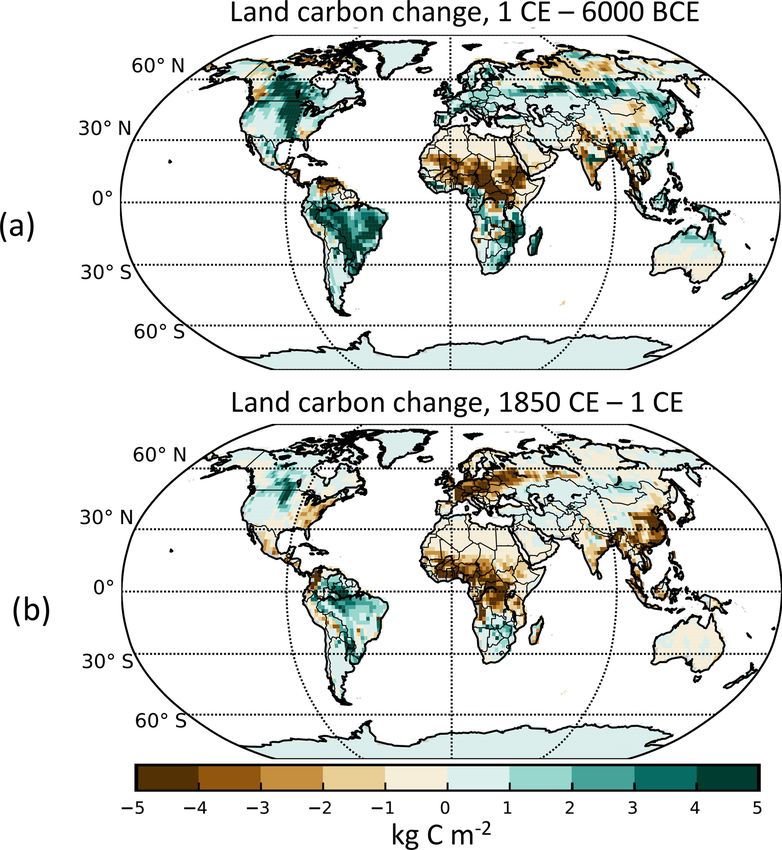
V. Brovkin et al.: What was the atmospheric CO2 source in the Holocene?                                                      2545

                                                                    ice-core reconstructions. Consequently, land and ocean car-
                                                                    bon uptakes do not interfere with each other, and the total
                                                                    mass of carbon in the land–ocean–atmosphere system is not
                                                                    conserved.
                                                                       The second transient simulation, TRAFc, started from the
                                                                    end of the 8KAFc simulation in the interactive climate–
                                                                    carbon cycle mode. Using equilibrium initial conditions and
                                                                    boundary conditions for the carbon cycle does not guaran-
                                                                    tee that the interactively simulated atmospheric CO2 con-
                                                                    centration will follow the trend reconstructed from ice cores.
                                                                    If the simulated atmospheric CO2 concentration differs sub-
                                                                    stantially from reconstructed data, both climate and carbon
                                                                    cycle components deviate from results which would be ob-
                                                                    tained if the model were driven by the reconstructed CO2
                                                                    forcing, and these biases complicate the comparison of trends
                                                                    between the model and observations. To ensure that simu-
                                                                    lated CO2 is close to the reconstructed time series, in the
                                                                    TRAFc simulation we used a CO2 nudging technique fol-
                                                                    lowing the approach of Gonzales and Ilyina (2016), target-
                                                                    ing the atmospheric CO2 record from ice-core reconstruc-
                                                                    tions. If the simulated atmospheric CO2 dropped below the
                                                                    target, the surface ocean total alkalinity and dissolved inor-
                                                                    ganic carbon (DIC) concentrations were decreased in a 2 : 1
                                                                    ratio to mimic the process of CaCO3 sedimentation. If CO2
                                                                    was higher than the target, the alkalinity and DIC were not
                                                                    changed. This alkalinity-forced approach is supported by ev-
Figure 1. Time series of applied forcings: (a) June–July–August     idence of decreasing deep ocean carbonate ion concentration
insolation at 60◦ N (W m−2 ), (b) atmospheric CO2 concentration     in the course of the Holocene (Yu et al., 2014) and excessive
(ppm), and (c) N2 O and CH4 concentrations (ppb). (d) Aerosol op-   coral reef buildup on shelves during deglaciation (Opdyke
tical depth of volcanic eruptions and (e) global area of crop and   and Walker, 1992; Vecsei and Berger, 2004) as well as recent
pastures (106 km2 ).
                                                                    synthesis by Cartapanis et al. (2018). The alkalinity decline
                                                                    resembles excessive shallow-water carbonate sedimentation
     Throughout the equilibration process, weathering               such as coral reefs, which are not included in HAMOCC.
     fluxes and CaCO3 content in sediments have been                   HAMOCC includes a module of sediment processes
     changed, which led to changes in total alkalinity              (Heinze et al., 1999). Interactive simulation of the sedi-
     (TA). This would have occurred naturally, with-                ment porewater chemistry and accumulation of solid sedi-
     out leading to excess TA, had the biogeochemistry              ment components, such as CaCO3 , particulate organic car-
     model been given a long enough spin-up time to                 bon (POC), opal, and clay, is a necessary condition to cal-
     equilibrate its sediments. Along with change in TA,            culate changes in the ocean biogeochemistry on millennial
     also DIC changed (with the molar ratio 2 : 1) in or-           timescales. To compensate for the POC, CaCO3 , and opal
     der to maintain the correct pCO2 .                             losses due to sedimentation, the fluxes into the sediment over
                                                                    the last 300 years of the spin-up runs were analysed, and a
   In the interactive carbon spin-up, the model firstly used the    globally uniform weathering input for silicate, alkalinity, nu-
same weathering rates as in 8KAF for ∼ 300 years, then it           trients in the form of organic matter, and dissolved inorganic
stabilized the system by increasing all the weathering fluxes       carbon was prescribed. Note that the weathering flux calcu-
(Si, organic matter, CaCO3 ), which led to a stabilization of       lated using this approach is sensitive to changes in the model
the surface alkalinity; afterwards the alkalinity changed to        setups (prescribed versus interactive CO2 ). This explains the
keep the target pCO2 . For the last few hundred years, weath-       difference between weathering fluxes in TRAF and TRAFc
ering was adjusted, which led to alkalinity stabilization. In       experiments (Table 1).
total, the 8KAFc spin-up took more than 1000 model years.
   We performed two transient simulations from 6000 BCE
to 1850 CE, a commonly defined onset of the industrial pe-
riod. The first transient simulation, TRAF, was initiated from
the end of the spin-up simulation 8KAF. In the TRAF simu-
lation, the atmospheric CO2 concentration is prescribed from

www.biogeosciences.net/16/2543/2019/                                                       Biogeosciences, 16, 2543–2555, 2019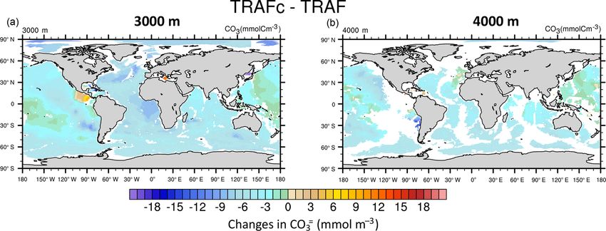
2546 V. Brovkin et al.: What was the atmospheric CO2 source in the Holocene?
Table 1. Changes in compartments and cumulative fluxes at 1850 CE relative to 6000 BCE (PgC).
Experiment Atmosphere Land Ocean, Ocean sediments, Surface ocean Ocean–atmosphere Land–ocean
water CaCO3 /Corg CaCO3 removal flux flux (weathering∗ )
TRAF 53 −39 −1324 2628/985 0 −152 2137
TRAFc 56 −17 −1799 2738/1068 1224 39 3270
TRAFc−TRAF 3 22 −475 110/83 1224 191 1133
The weathering flux is not accounted for in the land compartment changes (second column).
3 Results and discussion
3.1 Global response
The setup of the TRAF simulation resembles experiments
performed in CMIP5 with CO2 concentrations prescribed
from Representative Concentration Pathway (RCP) scenar-
ios. Similar to the RCP simulations, changes in carbon pools
on land and in the ocean could be estimated from land–
atmosphere and ocean–atmosphere fluxes, respectively. Cu-
mulative changes in the ocean and land CO2 fluxes reveal
that, by the end of the simulation, the ocean is a sink of
152 PgC, while the land is a source of 39 PgC (Fig. 2a, Ta-
ble 1). Accounting for an increase in the atmospheric car-
bon pool by 53 PgC, the total carbon budget has a deficit of
166 PgC by 1850 BCE (Fig. 3). Assuming that the CO2 air-
borne fraction on a millennial timescale is about one-sixth
(Maier-Reimer and Hasselmann, 1987), or even less if we
account for the land response due to CO2 fertilization, the
atmospheric CO2 concentration by the end of the simulation
would be 11–13 ppm less than observed (286 ppm). There-
fore, carbon budget changes in the TRAF experiment imply
that other boundary conditions are necessary to obtain the
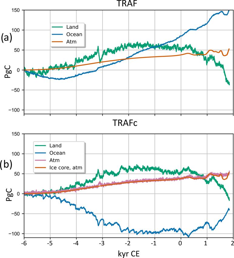
amplitude of the simulated CO2 concentration trend as re- Figure 2. Changes in the cumulative fluxes for major carbon cycle
constructed from the ice cores. components (land, ocean, and atmosphere) (PgC), from 6000 BCE
to 1850 CE in the TRAF (a) and TRAFc (b) simulations. The colour
Carbon cycle changes in the interactive CO2 simulation
legend is as follows: land is denoted in cyan, ocean in blue, atmo-
TRAFc are shown in Fig. 2b. At the beginning of the sim-
sphere in magenta, and ice-core reconstruction in orange.
ulation (during 6 to 5000 BCE), atmospheric CO2 and land
carbon fluctuate with an amplitude of several PgC, while the
ocean becomes a small source of CO2 to the atmosphere. Be-
tween 5000 and 2000 BCE, atmospheric carbon storage in- system (Pongratz et al., 2011), and external forcing scenar-
creases by about 30 PgC, and the land takes about 60 PgC ios, such as an abrupt reforestation of tropical America (Ka-
due to CO2 fertilization, while the ocean releases ca. 90 PgC. plan et al., 2011), might need to be accounted for.
Between 2000 BCE and 1 CE (start of the Common Era; note Decadal-scale excursions in ocean and land carbon stor-
that the year 0 does not exist in the CE system), land is a ages in Fig. 2b are mainly explained by responses to surface
source of 10 PgC to the atmosphere. After 1 CE, land carbon cooling resulting from volcanic eruptions. The most visible
losses accelerate due to land use changes, and by 1850 CE example of this CO2 response is during the period around
land carbon decreases by an additional 60 PgC. In 1850 CE, 3200 BCE, when reconstructed aerosol optical depth shows
the land and ocean are sources of 17 and 39 PgC, respec- an enhancement which is moderate in magnitude but is of
tively, while the atmosphere gains 56 PgC. The atmospheric long duration (Fig. 1d), potentially resulting from a long-
minimum in CO2 around 1600 CE apparent in the recon- duration high-latitude eruption or from contamination of the
struction is not reproduced by the model, confirming that the volcanic record by biogenic sulfate (Zielinski et al., 1994).
abrupt uptake of carbon by land or ocean is difficult to at- In response to this applied forcing, the land takes up carbon
tribute to internal variability in the coupled climate–carbon due to decreased respiration (see, for example, Brovkin et al.,
Biogeosciences, 16, 2543–2555, 2019 www.biogeosciences.net/16/2543/2019/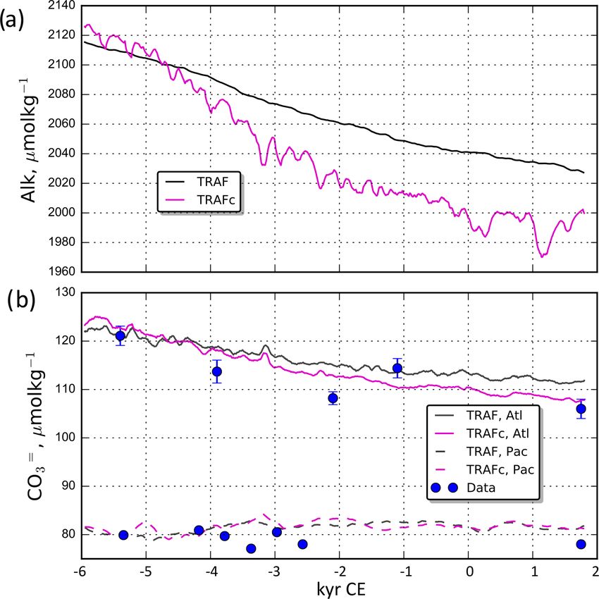
V. Brovkin et al.: What was the atmospheric CO2 source in the Holocene?                                                        2547

2010; Segschneider et al., 2013), while the alkalinity adjust-     3.2   Land carbon and vegetation
ment in the ocean counteracts the land carbon uptake, lead-
ing to carbon release from the ocean. After a few decades, the     Natural changes in vegetation and tree cover are most pro-
land turns into a source of carbon due to reduced productiv-       nounced for the period before 1 CE, before the start of sub-
ity, ocean carbon uptake restores, and atmospheric CO2 re-         stantial land use forcing. Comparing with 6000 BCE, veg-
veals a spike due to an excessive land source. At 3000 BCE,        etation cover becomes much less dense in Africa, mainly
this spike ceases, and the simulated CO2 continues to fluc-        due to decreased rainfall in response to the decreasing sum-
tuate around the ice-core time series. Although the volcanic       mer radiation in the Northern Hemisphere (Fig. 5a). Boreal
forcing included in the simulations at 3200 BCE is likely an       forests moved southward in both North America and Eurasia
overestimate, this case illustrates the response of the climate–   (Fig. 5b). The southward shift of vegetation in North Africa,
carbon system to an extreme volcanic aerosol forcing, which        and of the treeline in Eurasia from the mid-Holocene to the
leads to pronounced cooling of the land and ocean surfaces.        pre-industrial period, as well as the increase in vegetation and
   Changes in carbon density on land and in the ocean in           tree cover in central North America, is in line with pollen ev-
the course of both TRAF (not shown) and TRAFc simu-                idence (Prentice et al., 2000). The southward retreat of the
lations reveal complex patterns (Fig. 4). In the ocean, the        boreal forest in North America is much less pronounced than
vertically integrated DIC is decreasing everywhere, causing        in Eurasia (Fig. 5b). This is also in line with reconstructions,
negative change patterns dominating in the Southern Ocean          as there is no evidence for a significant shift of the treeline in
and North Pacific. Carbon sedimentation is high in upwelling       North America (Bigelow et al., 2003), likely due to the cool-
zones, mainly in coastal areas and the tropical Pacific, and       ing effects of the remains of the Laurentide ice sheet, which
that causes strong accumulation patterns. These sedimenta-         is not accounted for as a forcing in our simulations.
tion patterns are typical for the HAMOCC model with in-               Simulated changes in vegetation cover are reflected in the
teractive sediments (Heinze et al., 1999); they are generally      carbon density changes (Fig. 6a). From 6000 BCE to 1 CE,
well comparable with observed sedimentation patterns for or-       the carbon density decreases in North Africa, East Asia,
ganic carbon and CaCO3 (Seiter et al., 2004; Archer, 1996).        northern South America and above 60◦ N slightly in Eura-
The land has a mixed pattern of increased carbon density,          sia. In most of the rest of the land ecosystems, the carbon
mostly in South America and in central North America, with         density increases, mostly due to CO2 fertilization effects
decreased densities in Africa and East Asia. This is caused        as the atmospheric CO2 concentration increases by about
by an interplay between climate, CO2 , and land use effects        15 ppm by 1 CE. A strong increase in the Southern Hemi-
on soil and biomass storages.                                      sphere and central North America is also due to increased
   Changes in the carbon budget components over the exper-         vegetation density. After 1 CE, land carbon declines due to
imental period are provided in Table 1 and Fig. 3. For the         land use changes, predominantly deforestation (Fig. 6b). Pat-
atmosphere, the difference between the TRAF and TRAFc              terns of carbon decrease after 1 CE reflect land use patterns
simulations is minor (3 PgC). For the land, a difference of        except in South America, southern Africa, and central North
22 PgC is caused mainly by the relatively higher CO2 con-          America. The simulated increase in land carbon storage be-
centration in the TRAFc simulation, especially during the pe-      fore 2000 CE and decrease afterwards is consistent with the
riod of lower CO2 around 1600 CE, due to the CO2 fertiliza-        changes in atmospheric δ 13 CO2 (Elsig et al., 2009; Schmitt et
tion effect on the plant productivity. The ocean–atmosphere        al., 2012). The deconvolution approach (Fig. 3 in Elsig et al.,
cumulative fluxes (−152 and 39 PgC for TRAF and TRAFc,             2009) resulted in the land uptake of ca. 140 PgC from 6000
respectively) are minor in comparison with the ocean car-          to 3000 BCE, divided rather equally into ca. 70 PgC from
bon budget components, and the difference of 191 PgC is            6000 to 5000 BCE and 70 PgC between 5000 and 3000 BCE.
explained by the applied surface alkalinity removal in the         The 70 PgC uptake from 6000 to 5000 BCE deduced from
TRAFc simulation. The carbon inventory of the water col-           the increase in atmospheric δ 13 CO2 is not reproduced in
umn that predominantly includes dissolved inorganic car-           our experiments, likely because it is a non-equilibrium land
bon (DIC) loses 1324 and 1799 PgC in the TRAF and                  response which can be captured only in transient simula-
TRAFc runs, respectively. Sediments accumulate more than           tions during the last deglaciation. In our TRAF and TRAFc
3500 PgC in the form of CaCO3 and organic carbon, mainly           experiments, land accumulates about 60 PgC between 5000
compensated by the weathering flux from land. In the TRAFc         and 2000 BCE, comparable with land uptake of 70 PgC be-
experiment, 1224 PgC was removed from the ocean surface            tween 5000 and 3000 BCE inferred by Elsig et al. (2009).
in the form of CaCO3 , effectively reducing the weather-           We can conclude that after 5000 BCE, the land carbon dy-
ing flux (3270 PgC) to a scale below the TRAF experiment           namics in MPI-ESM (uptake of 60 PgC by 2000 BCE, release
(2137 PgC). In total, despite large changes in the cumulative      of 80–100 PgC by 1850 CE, predominantly due to land use)
fluxes of weathering and sedimentation, the net cumulative         is similar to the land carbon changes estimated by Elsig et
ocean–atmosphere flux is minor.                                    al. (2009).

www.biogeosciences.net/16/2543/2019/                                                       Biogeosciences, 16, 2543–2555, 2019
2548                                                V. Brovkin et al.: What was the atmospheric CO2 source in the Holocene?

Figure 3. Changes in the carbon cycle compartments (land, ocean, and atmosphere) (PgC), and cumulative fluxes between them (PgC), from
6000 BCE to 1850 CE in the TRAF (a) and TRAFc (b) simulations. Flux from the lithosphere include weathering (TRAF) and weathering
minus shallow-water sedimentation (TRAFc). Carbon budget has a negative 166 Pg disbalance in the TRAF simulation, while it is closed in
the TRAFc run.

Figure 4. Combined map of changes in the ocean carbon storage
(vertically integrated ocean water column plus sediments minus
weathering) and land (soil plus vegetation) at the end of the TRAFc
simulation (1850 CE) relative to 6000 BCE (in kgC m−2 ).

3.3    Ocean carbon

Simulated physical ocean fields, including sea surface tem-
peratures and the Atlantic meridional overturning, do not
change substantially in the Holocene. The main reason for
the declining carbon storage in the water column (Fig. 4, Ta-
ble 1) is a decrease in ocean alkalinity (Figs. 7a; 8a). This         Figure 5. Change in vegetation fraction (a) and tree cover frac-
is explained by the applied surface ocean alkalinity forcing          tion (b) at 1 CE relative to 6000 BCE in the TRAFc simulation.
and also by the response of the ocean carbonate chemistry to
changes in carbonate production. The global CaCO3 export
from the surface to the aphotic layer increases by about 5 %          two simulations by 1850 CE is 35 µmol kg−1 , similar to the
between 6000 and 2000 BCE in both TRAF and TRAFc sim-                 difference in surface alkalinity changes shown in Fig. 7a. Ac-
ulations and returns to the 6000 BCE level by the end of the          counting for 7850 years of experimental length, the alkalinity
simulation. Comparing TRAF and TRAFc simulations, the                 loss corresponds to 8.2 and 11.2 Tmol yr−1 CaCO3 sedimen-
difference in the globally averaged ocean alkalinity in these         tation in TRAF and TRAFc simulations, respectively. The re-

Biogeosciences, 16, 2543–2555, 2019                                                        www.biogeosciences.net/16/2543/2019/
V. Brovkin et al.: What was the atmospheric CO2 source in the Holocene?                                                          2549

                                                                   Figure 7. (a) 100-year moving average of global surface alkalin-
                                                                   ity, µmol kg−1 . (b) 100-year moving average of carbonate ion con-
Figure 6. Change in land carbon density (kg C m−2 ), relative to   centration (µmol kg−1 ), averaged for nine neighbouring model grid
6000 BCE at 1 CE (a) and at 1850 CE relative to 1 CE (b) in the    cells centred in the deep Atlantic (12◦ N, 60◦ W; 3400 m) and deep
TRAFc simulation.                                                  Pacific (1◦ S, 160◦ W; 3100 m). The data (circles) are [CO=3 ] for
                                                                   sites VM28-122 and GGC48 reconstructed by Yu et al. (2013),
                                                                   which appropriately correspond to the ocean grid cells accounting
                                                                   for the model bathymetry mask. Data uncertainties (1σ ) reported
quired excessive carbonate sedimentation in the shallow wa-
                                                                   for the Atlantic by Yu et al. (2013) are indicated by whiskers. 35 ‰
ters would be 3 Tmol yr−1 in TRAFc relative to TRAF, or at         salinity is used for model unit conversion from m−3 to kg−1 .
the lower bound of estimates of 3.35 to 12 Tmol yr−1 CaCO3
accumulation proposed by Vecsei and Berger (2004) and
Opdyke and Walker (1992). Even corresponding excessive             and Clark (2007) suggested a similar amplitude of [CO=3 ]
carbonate sedimentation of 11.2 Tmol yr−1 CaCO3 in the             changes in the deep Atlantic. Comparison of changes in
TRAFc simulation would fall into this observational range,         [CO=3 ] in TRAF and TRAFc simulations with [CO=3 ] data re-
although at the higher bound. Let us note that in the 8KAF         constructed by Yu et al. (2013) reveals a significant differ-
and TRAF experiments the weathering was not adjusted to            ence between TRAF and TRAFc in the Atlantic (Fig. 7b).
changes in boundary conditions, and this likely caused sur-        Decrease in [CO=3 ] in the TRAFc simulation is more sig-
face alkalinity decrease in the transient run (Fig. 7c). In        nificant than in the TRAF experiment, presumably due to a
particular, this alkalinity drift in TRAF explains the initial     stronger decrease in alkalinity in the former simulation. In-
decrease in the ocean carbon storage until ca. 4500 BCE            terestingly, changes in [CO=3 ] at the Pacific site are not sig-
(Fig. 2a), despite an increase in atmospheric CO2 concen-          nificant in both simulations, while the data propose a slight
tration. If TRAF had started from an equilibrated system as        decrease in carbonate ion concentration. The difference be-
TRAFc did, the beginning of TRAF would have been more              tween the Atlantic and Pacific responses is visible in Fig. 8.
similar to TRAFc, and the ocean carbon uptake would have           In both experiments, simulated changes in [CO=3 ] in the At-
started earlier.                                                   lantic and Southern Ocean are stronger than in the Indo-
   Besides the estimate of applied carbonate accumulation          Pacific. At a depth of 4 km, comparable with the depth of the
forcing, another way to address the plausibility of simu-          cores by Broecker and Clark (2007), changes in the tropical
lated alkalinity trends is to compare changes in the carbonate     oceans in both simulations are in the range of 0–15 mol m−3 .
ion concentration ([CO=3 ]) in the deep Atlantic and Pacific       Changes in the TRAFc experiment are more pronounced than
Ocean with available reconstructions of carbonate ion con-         in TRAF due to stronger changes in alkalinity. As expected,
centrations. Using the benthic foraminiferal B/Ca proxy for        [CO=3 ] changes are more pronounced for depths of 3 km than
deep water [CO=3 ], Yu et al. (2014) found that [CO=3 ] in the     for 4 km (Fig. 8).
deep Indian and Pacific Ocean declined by 5–15 µmol kg−1
during the Holocene. Broecker et al. (1999) and Broecker

www.biogeosciences.net/16/2543/2019/                                                        Biogeosciences, 16, 2543–2555, 2019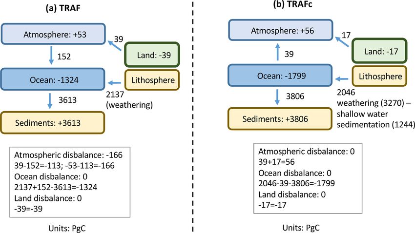
2550                                             V. Brovkin et al.: What was the atmospheric CO2 source in the Holocene?

Figure 8. Differences in carbonate ion concentration (mmol m−3 ), between TRAFc and TRAF simulations in 1850 CE at the depth of
3 km (a) and 4 km (b).

   Comparison of simulated ocean carbon budget with re-           compensate for the peatland growth, for example, emissions
cent carbon data synthesis (Cartapanis et al., 2018) is shown     due to ongoing thermokarst formation and erosion of per-
in Table 2. In comparison with mean data values, CaCO3            mafrost soils, especially close to the Arctic coast (Lindgren
burial in the model (27.9–29.1, plus 13 TmolC yr−1 surface        et al., 2018). Secondly, HAMOCC does not include coral
removal in the TRAFc experiment) is higher than in the            reefs as a process-based component. This is one of the rea-
data (23.3 TmolC yr−1 ); however, this is compensated by          sons why the surface alkalinity was forced directly in the
a higher modelling weathering rate (24.6–34.7 TmolC yr−1 )        TRAFc simulation. Thirdly, the applied versions of JSBACH
compared to 11.7 TmolC yr−1 in the data. The model val-           and HAMOCC do not simulate carbon isotope changes, in
ues are at the upper end of the data uncertainty range            particular 13 C changes. For land carbon, the increase in the
(11–38 TmolC yr−1 ; see min–max range for CaCO3 sedi-             carbon storage on land by 50–60 PgC by 2000 BCE and its
mentation in Table 2). Organic carbon burial in the model         decrease by 80 PgC by 1850 CE would be translated into
(10.5–11.3 Tmol yr−1 ) is less than in the averaged data          a ca. 0.05 ‰ decrease in atmospheric δ 13 CO2 . This small
(18.3 Tmol yr−1 ); however, the uncertainty in the burial is so   change is within the uncertainty bounds of δ 13 CO2 recon-
high (6–58 Tmol yr−1 ) that the model values are almost twice     structed from ice cores (Elsig et al., 2009; Schmitt et al.,
more than the lower end of the data range.                        2012). For ocean carbon, carbonate changes would not sig-
   An important question is whether the ocean on average lost     nificantly modify the ocean and atmospheric δ 13 CO2 content.
carbon content over the Holocene. In equilibrium, volcanic        Simulated changes in biological production and export flux
CO2 outgassing (not accounted for explicitly in the model),       might have affected the atmospheric δ 13 CO2 , but the scale
both aerial and submarine, compensates for weathering;            will likely be small.
therefore for proper comparison it needs to be included in the       In addition, two limitations are intrinsic to the setups of
table as the ocean–atmosphere budget. In that case, averaged      spin-up and transient simulations. Firstly, assuming that all
ocean water column losses in the data are 20.8 TmolC yr−1 .       carbon cycle components are initially in equilibrium with
Similar to the data, the model shows the loss of carbon from      boundary conditions is a simplification. Changes in climate
the water column, 13.8 and 18.7 TmolC yr−1 in the TRAF            due to slowly changing boundary conditions, such as orbital
and TRAFc experiments, respectively. Therefore, simulated         or greenhouse gas forcing, are occurring on timescales simi-
ocean carbon losses are qualitatively (and even quantitatively    lar to long-term processes in the carbon system (soil buildup
for TRAFc) in line with observations.                             on land, carbonate compensation in the ocean). Therefore,
                                                                  the carbon cycle is never in full equilibrium, and memory
3.4    Limitation of the model setup                              in the carbon cycle processes, due for example to carbonate
                                                                  compensation in the ocean during deglaciation, affects the
There are certain limitations of the carbon cycle models used     carbon dynamics afterwards. A proper way to account for the
in the study. Firstly, the applied version of JSBACH does not     memory effect is to set spin-up simulations millennia before
include wetland and peatland processes. If the Holocene peat      the Holocene, e.g. at the last glacial maximum (19 000 BCE),
accumulation of several hundred gigatonnes of carbon (GtC;        and perform a transient deglaciation simulation. Simulations
Yu, 2012) were accounted for, the land would be a stronger        with intermediate complexity models suggested that the im-
sink of carbon during 6000 to 2000 BCE. This might require        pact of the memory effect from deglaciation on Holocene
an even stronger ocean source. On the other hand, we neglect      carbon dynamics, in particular due to carbonate compensa-
other sources of atmospheric CO2 which might at least partly      tion, is significant (e.g. Menviel and Joos, 2012). However,

Biogeosciences, 16, 2543–2555, 2019                                                   www.biogeosciences.net/16/2543/2019/
V. Brovkin et al.: What was the atmospheric CO2 source in the Holocene? 2551
Table 2. Model–data comparison of average carbon fluxes from 6000 BCE to 1850 CE (Tmol yr−1 ).
Source CaCO3 Surface CaCO3 Corg Volcanic Weathering Ocean, water
burial removal burial outgassinga column losses
Datab average (min–max) 23.3 (11–38) 0 18.3 (6–58) 9.2 (4–15) 11.7 (9–19) 20.8c
TRAF 27.9 0 10.5 0 24.6 13.8
TRAFc 29.1 13 11.3 0 34.7 18.7
a Including aerial volcanic CO outgassing. b Pre-industrial fluxes according to the Fig. 1 in Cartapanis et al. (2018). c Subtracting volcanic outgassing.
2
transient deglaciation run is presently too challenging for ulation with interactive CO2 is performed in the nudging
full-scale ESMs due to high computational costs. Secondly, mode: we use the surface alkalinity changes as the forcing
the weathering fluxes are assumed to be constant during the for ocean–atmosphere CO2 flux. In response to this forcing,
transient simulation. While this is a common practice for the ocean serves as a source of carbon over the Holocene. The
ocean biogeochemistry simulations (e.g. Ilyina et al., 2013; alkalinity decline is within the bounds of proposed changes
Heinze et al., 2016), it results in a mismatch between weath- in the carbonate sedimentation in shallow waters and consis-
ering and sedimentation under changing boundary conditions tent with available proxies for carbonate ion decrease in the
in transient simulations. As land climate evolves, weathering deep sea.
fluxes are changing due to their dependence on runoff and There are several limitations of our simulations related to
temperature. This causes a shift in land–ocean fluxes of car- initial conditions and forcings. We cannot simply overcome
bon, alkalinity, and nutrients, leading to inventory changes them by repeating runs in a different setup or by doing addi-
and a possible drift in ocean–atmosphere fluxes. In particu- tional sensitivity experiments due to the high computational
lar, as POC fluxes to the sediment are not properly compen- costs of full-scale ESMs. Despite these limitations, we can
sated by the fixed weathering, this leads to changes in nutri- make several conclusions on the potential source of CO2 to
ent inventory in transient simulations. Both CaCO3 and POC the atmosphere during the last 8000 years. Regarding the
fluxes to sediments are changing with time; this also leads to land source, experiments demonstrate that natural carbon dy-
changes in the rain ratio. In the absence of factorial experi- namics led to an increase in the land carbon storage during
ments without these changes, it is difficult to infer how these the first half of the simulation (until 2000 BCE). This is in
trends in nutrients and biogenic opal and carbonate fluxes af- line with previous simulations performed with intermediate
fect atmospheric CO2 . These two caveats (steady-state initial complexity models (e.g. Kaplan et al., 2002; Kleinen et al.,
conditions and fixed weathering) apply to both TRAF and 2016) and with ice-core deconvolution studies (Elsig et al.,
TRAFc simulations. Consequently, to simulate the carbon 2009; Schmitt et al., 2012). During 6000 to 2000 BCE, the at-
budget correctly, models have to include interactive weath- mospheric CO2 increase is about two-thirds of the estimated
ering processes. 20 ppm increase. Although the TRAF and TRAFc simula-
tions do not account for land use changes during this pe-
riod, assuming that land use was a source of carbon to the
4 Conclusions atmosphere requires about 100 PgC to compensate for nat-
ural land, ocean, and atmospheric carbon content increase
Using the Earth system model MPI-ESM-LR, we performed during this time. If we account for the peat carbon accumu-
two transient simulations of the climate and carbon cycle dy- lation (neglected in TRAFc), emissions from land use would
namics in the Holocene, one with prescribed atmospheric need to be higher (about 200 PgC over the period 6000 to
CO2 and one with interactive CO2 using nudged ocean al- 2000 BCE). This is not absolutely impossible (Kaplan et al.,
kalinity. In both simulations, the land is a carbon sink during 2011), but such a high-end land use emission scenario for
the mid-Holocene (from 6000 to 2000 BCE) and a source of the end of the Neolithic period, when agriculture was not yet
CO2 after 1 CE due to land use changes. Changes in vegeta- widespread in Europe and America, is rather unlikely.
tion cover at 6000 BCE relative to 1 CE (enhanced vegetation Regarding the ocean source, both TRAF and TRAFc sim-
cover in North Africa, northward extension of boreal forest ulations show a decrease in ocean alkalinity. Even if this de-
in Asia) are in line with available pollen records. crease is a result of a drift in the carbonate system due to
In the prescribed CO2 experiment TRAF, the ocean is a imperfect initialization of the balance between sedimentation
sink of carbon. This strengthens the argument that neither and weathering, in both simulations the model is capable of
changes in circulation nor in sea surface temperatures are ca- producing a decrease in the carbonate ion concentrations in
pable of explaining CO2 growth in the Holocene. In the cou- the Atlantic, which is in the direction proposed by proxy data
pled land–ocean–atmosphere system, there is a total deficit (Fig. 8b). The magnitude of the decrease in the TRAF exper-
of 166 PgC by the end of the experiment. The TRAFc sim- iment is underestimated compared to the proxy data, while it
www.biogeosciences.net/16/2543/2019/ Biogeosciences, 16, 2543–2555, 20192552 V. Brovkin et al.: What was the atmospheric CO2 source in the Holocene?
is in line with the data for the TRAFc experiment. As land Review statement. This paper was edited by Christoph Heinze and
serves as a carbon sink until 2000 BCE due to natural (non- reviewed by Fortunat Joos and one anonymous referee.
anthropogenic) carbon cycle processes in both experiments,
the missing source of carbon for land and atmosphere could
only be attributed to ocean. Within our model framework, an
additional mechanism is required for consistency with ice- References
core CO2 data, such as surface alkalinity decrease, due, for
example, to unaccounted for carbonate accumulation pro- Archer, D.: A data-driven model of the global calcite lysocline,
cesses on shelves supported by observational evidence. Fi- Global Biogeochem. Cy., 10, 511–526, 1996.
nally, our simulations support the hypothesis that the ocean Bader, J., Jungclaus, J., Krivova, N., Lorenz, S., Maycock, A., Rad-
was a source of CO2 until the late Holocene when anthro- datz, T., Schmidt, H., Toohey, M., Wu, C.-J., and Claussen, M.:
pogenic CO2 sources started to affect atmospheric CO2 . Global temperature modes shed light on the Holocene tempera-
ture conundrum, Nat. Commun., submitted, 2019.
Baker, J. L., Lachniet, M. S., Chervyatsova, O., Asmerom, Y., and
Code and data availability. The model code is available after re- Polyak, V. J.: Holocene warming in western continental Eurasia
quest and after acceptance of the MPG license. The data used for driven by glacial retreat and greenhouse forcing, Nat. Geosci.,
the analysis and figures are available from the MPI-M library by 10, 430–435, https://doi.org/10.1038/ngeo2953, 2017.
contacting publications@mpimet.mpg.de. Berger, A. L.: Long-term variations of daily insolation and quater-
nary climatic changes, J. Atmos. Sci., 35, 2362–2367, 1978.
Bigelow, N. H., Brubaker, L. B., Edwards, M. E., Harrison, S.
P., Prentice, I. C., Anderson, P. M., Andreev, A. A., Bartlein,
Author contributions. TR and IS contributed to the model develop-
P. J., Christensen, T. R., Cramer, W., Kaplan, J. O., Lozhkin,
ment and experimental setup. TI and MC contributed to the exper-
A. V., Matveyeva, N. V., Murray, D. F., McGuire, A. D., Raz-
imental design of the simulations, MT provided volcanic forcing,
zhivin, V. Y., Ritchie, J. C., Smith, B., Walker, D. A., Gajew-
SL performed the simulations, and VB analysed the simulations and
ski, K., Wolf, V., Holmqvist, B. H., Igarashi, Y., Kremenet-
wrote the first draft. All authors contributed to the result discussion
skii, K., Paus, A., Pisaric, M. F. J., and Volkova, V. S.: Cli-
and manuscript writing.
mate change and Arctic ecosystems: 1. Vegetation changes
north of 55 degrees N between the last glacial maximum, mid-
Holocene, and present, J. Geophys. Res.-Atmos., 108, 8170,
Competing interests. The authors declare that they have no conflict https://doi.org/10.1029/2002jd002558, 2003.
of interest. Broecker, W. and Clark, E.: Is the magnitude of the carbonate ion
decrease in the abyssal ocean over the last 8 kyr consistent with
the 20 ppm rise in atmospheric CO2 content?, Paleoceanography,
Special issue statement. This article is part of the special issue 22, PA1202, https://doi.org/10.1029/2006pa001311, 2007.
“The 10th International Carbon Dioxide Conference (ICDC10) and Broecker, W. S., Clark, E., McCorkle, D. C., Peng, T. H., Hajdas,
the 19th WMO/IAEA Meeting on Carbon Dioxide, other Green- I., and Bonani, G.: Evidence for a reduction in the carbonate ion
house Gases and Related Measurement Techniques (GGMT-2017) content of the deep sea during the course of the Holocene, Pale-
(AMT/ACP/BG/CP/ESD inter-journal SI)”. It is a result of the 10th oceanography, 14, 744–752, 1999.
International Carbon Dioxide Conference, Interlaken, Switzerland, Broecker, W. S., Lynch-Stieglitz, J., Clark, E., Hajdas, I., and Bo-
21–25 August 2017. nani, G.: What caused the atmosphere’s CO2 content to rise dur-
ing the last 8000 years?, Geochem. Geophy. Geosy., 2, 1062,
https://doi.org/10.1029/2001GC000177, 2001.
Acknowledgements. This work contributes to the project PalMod, Brovkin, V., Bendtsen, J., Claussen, M., Ganopolski, A., Ku-
funded by the German Federal Ministry of Education and Re- batzki, C., Petoukhov, V., and Andreev, A.: Carbon cycle, veg-
search (BMBF), Research for Sustainable Development (FONA; etation, and climate dynamics in the Holocene: Experiments
https://www.fona.de, last access: 26 June 2019). We are grateful to with the CLIMBER-2 model, Global Biogeochem. Cy., 16, 1139,
the authors of the companion paper by Bader et al. (2019) for in- https://doi.org/10.1029/2001gb001662, 2002.
sightful discussions. We thank Mathias Heinze for helping with the Brovkin, V., Kim, J. H., Hofmann, M., and Schneider, R.:
equilibrium model spin-up, Veronika Gayler for post-processing the A lowering effect of reconstructed Holocene changes
model output, and Estefania Montoya-Duque for archiving the pri- in sea surface temperatures on the atmospheric CO2
mary data. concentration, Global Biogeochem. Cy., 22, Gb1016,
https://doi.org/10.1029/2006gb002885, 2008.
Brovkin, V., Raddatz, T., Reick, C. H., Claussen, M., and
Financial support. The article processing charges for this open- Gayler, V.: Global biogeophysical interactions between
access publication were covered by the Max Planck Society. forest and climate, Geophys. Res. Lett., 36, L07405,
https://doi.org/10.1029/2009gl037543, 2009.
Brovkin, V., Lorenz, S. J., Jungclaus, J., Raddatz, T., Timm-
reck, C., Reick, C. H., Segschneider, J., and Six, K.: Sensitiv-
ity of a coupled climate-carbon cycle model to large volcanic
Biogeosciences, 16, 2543–2555, 2019 www.biogeosciences.net/16/2543/2019/V. Brovkin et al.: What was the atmospheric CO2 source in the Holocene? 2553 eruptions during the last millennium, Tellus B., 62, 674–681, A., Jones, C. D., Kindermann, G., Kinoshita, T., Goldewijk, K. https://doi.org/10.1111/j.1600-0889.2010.00471.x, 2010. K., Riahi, K., Shevliakova, E., Smith, S., Stehfest, E., Thomson, Brovkin, V., Bruecher, T., Kleinen, T., Zaehle, S., Joos, F., Roth, A., Thornton, P., van Vuuren, D. P., and Wang, Y. P.: Harmoniza- R., Spahni, R., Schmitt, J., Fischer, H., Leuenberger, M., Stone, tion of land-use scenarios for the period 1500–2100: 600 years E. J., Ridgwell, A., Chappellaz, J., Kehrwald, N., Barbante, C., of global gridded annual land-use transitions, wood harvest, Blunier, T., and Jensen, D. D.: Comparative carbon cycle dynam- and resulting secondary lands, Climatic Change, 109, 117–161, ics of the present and last interglacial, Quaternary Sci. Rev., 137, https://doi.org/10.1007/s10584-011-0153-2, 2011. 15–32, https://doi.org/10.1016/j.quascirev.2016.01.028, 2016. Ilyina, T., Six, K. D., Segschneider, J., Maier-Reimer, E., Li, Cartapanis, O., Galbraith, E. D., Bianchi, D., and Jaccard, S. L.: H., and Nunez-Riboni, I.: Global ocean biogeochemistry model Carbon burial in deep-sea sediment and implications for oceanic HAMOCC: Model architecture and performance as compo- inventories of carbon and alkalinity over the last glacial cycle, nent of the MPI-Earth system model in different CMIP5 ex- Clim. Past, 14, 1819–1850, https://doi.org/10.5194/cp-14-1819- perimental realizations, J. Adv. Model. Earth Sy., 5, 287–315, 2018, 2018. https://doi.org/10.1029/2012ms000178, 2013. Elsig, J., Schmitt, J., Leuenberger, D., Schneider, R., Eyer, Indermühle, A., Stocker, T. F., Joos, F., Fischer, H., Smith, H. J., M., Leuenberger, M., Joos, F., Fischer, H., and Stocker, Wahlen, M., Deck, B., Mastroianni, D., Tschumi, J., Blunier, T. F.: Stable isotope constraints on Holocene carbon cycle T., Meyer, R., and Stauffer, B.: Holocene carbon-cycle dynamics changes from an Antarctic ice core, Nature, 461, 507–510, based on CO2 trapped in ice at Taylor Dome, Antarctica, Nature, https://doi.org/10.1038/nature08393, 2009. 398, 121–126, 1999. Foley, J. A.: The sensitivity of the terrestrial biosphere to climatic Joos, F., Gerber, S., Prentice, I. C., Otto-Bliesner, B. L., change – a simulation of the middle Holocene, Global Bio- and Valdes, P. J.: Transient simulations of Holocene atmo- geochem. Cy., 8, 505–525, 1994. spheric carbon dioxide and terrestrial carbon since the Last Giorgetta, M. A., Jungclaus, J., Reick, C. H., Legutke, S., Bader, Glacial Maximum, Global Biogeochem. Cy., 18, GB2002, J., Bottinger, M., Brovkin, V., Crueger, T., Esch, M., Fieg, K., https://doi.org/10.1029/2003gb002156, 2004. Glushak, K., Gayler, V., Haak, H., Hollweg, H. D., Ilyina, T., Jungclaus, J. H., Fischer, N., Haak, H., Lohmann, K., Marotzke, Kinne, S., Kornblueh, L., Matei, D., Mauritsen, T., Mikolajew- J., Matei, D., Mikolajewicz, U., Notz, D., and von Storch, J. icz, U., Mueller, W., Notz, D., Pithan, F., Raddatz, T., Rast, S., S.: Characteristics of the ocean simulations in the Max Planck Redler, R., Roeckner, E., Schmidt, H., Schnur, R., Segschnei- Institute Ocean Model (MPIOM) the ocean component of the der, J., Six, K. D., Stockhause, M., Timmreck, C., Wegner, J., MPI-Earth system model, J. Adv. Model. Earth Sy., 5, 422–446, Widmann, H., Wieners, K. H., Claussen, M., Marotzke, J., and https://doi.org/10.1002/jame.20023, 2013. Stevens, B.: Climate and carbon cycle changes from 1850 to Kaplan, J. O., Prentice, I. C., Knorr, W., and Valdes, P. J.: 2100 in MPI-ESM simulations for the Coupled Model Intercom- Modeling the dynamics of terrestrial carbon storage since parison Project phase 5, J. Adv. Model. Earth Sy., 5, 572–597, the Last Glacial Maximum, Geophys. Res. Lett., 29, 2074, https://doi.org/10.1002/jame.20038, 2013. https://doi.org/10.1029/2002gl015230, 2002. Goll, D. S., Brovkin, V., Liski, J., Raddatz, T., Thum, T., and Todd- Kaplan, J. O., Krumhardt, K. M., Ellis, E. C., Ruddiman, W., and Brown, K. E. O.: Strong dependence of CO2 emissions from an- Klein Goldewijk, K.: Holocene carbon emissions as a result of thropogenic land cover change on initial land cover and soil car- anthropogenic land cover change, The Holocene, 21, 775–791, bon parametrization, Global Biogeochem. Cy., 29, 1511–1523, https://doi.org/10.1177/0959683610386983, 2011. https://doi.org/10.1002/2014gb004988, 2015. Kim, J. H., Rimbu, N., Lorenz, S. J., Lohmann, G., Nam, S. Gonzalez, M. F. and Ilyina, T.: Impacts of artificial ocean I., Schouten, S., Ruhlemann, C., and Schneider, R. R.: North alkalinization on the carbon cycle and climate in Earth Pacific and North Atlantic sea-surface temperature variabil- system simulations, Geophys. Res. Lett., 43, 6493–6502, ity during the holocene, Quaternary Sci. Rev., 23, 2141–2154, https://doi.org/10.1002/2016gl068576, 2016. https://doi.org/10.1016/j.quascirev.2004.08.010, 2004. Goodwin, P., Oliver, K. I. C., and Lenton, T. M.: Ob- Kleinen, T., Brovkin, V., and Munhoven, G.: Modelled interglacial servational constraints on the causes of Holocene carbon cycle dynamics during the Holocene, the Eemian and CO2 change, Global Biogeochem. Cy., 25, GB3011, Marine Isotope Stage (MIS) 11, Clim. Past, 12, 2145–2160, https://doi.org/10.1029/2010gb003888, 2011. https://doi.org/10.5194/cp-12-2145-2016, 2016. Hagemann, S. and Stacke, T.: Impact of the soil hydrology scheme Klein Goldewijk, K., Beusen, A., Doelman, J., and Stehfest, E.: An- on simulated soil moisture memory, Clim. Dynam., 44, 1731– thropogenic land use estimates for the Holocene – HYDE 3.2, 1750, https://doi.org/10.1007/s00382-014-2221-6, 2015. Earth Syst. Sci. Data, 9, 927–953, https://doi.org/10.5194/essd- Heinze, C., Maier-Reimer, E., Winguth, A. M. E., and Archer, 9-927-2017, 2017. D.: A global oceanic sediment model for long-term cli- Köhler, P.: Interactive comment on “What was the source of the mate studies, Global Biogeochem. Cy., 13, 221–250, atmospheric CO2 increase during the Holocene?” by V. Brovkin https://doi.org/10.1029/98gb02812, 1999. et al., Biogeosciences Discuss., https://doi.org/10.5194/bg-2019- Heinze, C., Hoogakker, B. A. A., and Winguth, A.: Ocean car- 64-SC1, 2019. bon cycling during the past 130 000 years – a pilot study on Krivova, N. A., Solanki, S. K., and Unruh, Y. C.: To- inverse palaeoclimate record modelling, Clim. Past, 12, 1949- wards a long-term record of solar total and spectral 1978, https://doi.org/10.5194/cp-12-1949-2016, 2016. irradiance, J. Atmos. Sol.-Terr. Phys., 73, 223–234, Hurtt, G. C., Chini, L. P., Frolking, S., Betts, R. A., Feddema, J., https://doi.org/10.1016/j.jastp.2009.11.013, 2011. Fischer, G., Fisk, J. P., Hibbard, K., Houghton, R. A., Janetos, www.biogeosciences.net/16/2543/2019/ Biogeosciences, 16, 2543–2555, 2019
2554                                                  V. Brovkin et al.: What was the atmospheric CO2 source in the Holocene?

Lindgren, A., Hugelius, G., and Kuhry, P.: Extensive loss of past       Ruddiman, W. F.: Geographic evidence of the early anthropogenic
  permafrost carbon but a net accumulation into present-day soils,         hypothesis, Anthropocene, 20, 4–14, 2017.
  Nature, 560,p. 219, https://doi.org/10.1038/s41586-018-0371-0,        Schmitt, J., Schneider, R., Elsig, J., Leuenberger, D., Lourantou,
  2018.                                                                    A., Chappellaz, J., Köhler, P., Joos, F., Stocker, T. F., Leuen-
Maier-Reimer, E. and Hasselmann, K.: Transport and                         berger, M., and Fischer, H.: Carbon isotope constraints on the
  storage of CO2 in the ocean – an inorganic ocean-                        deglacial CO2 rise from ice cores, Science, 336, 711–714,
  circulation carbon cycle model, Clim. Dynam., 2, 63–90,                  https://doi.org/10.1126/science.1217161, 2012.
  https://doi.org/10.1007/bf01054491, 1987.                             Schneider, R., Schmitt, J., Köhler, P., Joos, F., and Fischer, H.:
Marcott, S. A., Shakun, J. D., Clark, P. U., and Mix, A.                   A reconstruction of atmospheric carbon dioxide and its stable
  C.: A Reconstruction of Regional and Global Tempera-                     carbon isotopic composition from the penultimate glacial max-
  ture for the Past 11,300 Years, Science, 339, 1198–1201,                 imum to the last glacial inception, Clim. Past, 9, 2507–2523,
  https://doi.org/10.1126/science.1228026, 2013.                           https://doi.org/10.5194/cp-9-2507-2013, 2013.
Martin, J. H., Knauer, G. A., Karl, D. M., and Broenkow,                Segschneider, J., Beitsch, A., Timmreck, C., Brovkin, V., Ilyina,
  W. W.: VERTEX – carbon cycling in the northeast Pacific,                 T., Jungclaus, J., Lorenz, S. J., Six, K. D., and Zanchettin, D.:
  Deep-Sea Res. Pt. 1, 34, 267–285, https://doi.org/10.1016/0198-          Impact of an extremely large magnitude volcanic eruption on
  0149(87)90086-0, 1987.                                                   the global climate and carbon cycle estimated from ensemble
Menviel, L. and Joos, F.: Toward explaining the Holocene car-              Earth System Model simulations, Biogeosciences, 10, 669–687,
  bon dioxide and carbon isotope records: Results from transient           https://doi.org/10.5194/bg-10-669-2013, 2013.
  ocean carbon cycle-climate simulations, Paleoceanography, 27,         Seiter, K., Hensen, C., Schroter, E., and Zabel, M.: Or-
  PA1207, https://doi.org/10.1029/2011pa002224, 2012.                      ganic carbon content in surface sediments – defining re-
Monnin, E., Steig, E. J., Siegenthaler, U., Kawamura, K., Schwan-          gional provinces, Deep-Sea Res. Pt. I, 51, 2001–2026,
  der, J., Stauffer, B., Stocker, T. F., Morse, D. L., Barnola, J.         https://doi.org/10.1016/j.dsr.2004.06.014, 2004.
  M., Bellier, B., Raynaud, D., and Fischer, H.: Evidence for sub-      Stevens, B., Giorgetta, M., Esch, M., Mauritsen, T., Crueger, T.,
  stantial accumulation rate variability in Antarctica during the          Rast, S., Salzmann, M., Schmidt, H., Bader, J., Block, K.,
  Holocene, through synchronization of CO2 in the Taylor Dome,             Brokopf, R., Fast, I., Kinne, S., Kornblueh, L., Lohmann, U., Pin-
  Dome C and DML ice cores, Earth Planet. Sc. Lett., 224, 45–54,           cus, R., Reichler, T., and Roeckner, E.: Atmospheric component
  https://doi.org/10.1016/j.epsl.2004.05.007, 2004.                        of the MPI-M Earth System Model: ECHAM6, J. Adv. Model.
Opdyke, B. N. and Walker, J. C. G.: Return of the coral reef hy-           Earth Sy., 5, 146–172, https://doi.org/10.1002/jame.20015, 2013.
  pothesis: Basin to shelf partitioning of CaCO3 and its effect on      Stocker, B. D., Feissli, F., Strassmann, K. M., Spahni, R., and
  atmospheric CO2 , Geology, 20, 730–736, 1992.                            Joos, F.: Past and future carbon fluxes from land use change,
Paulsen, H., Ilyina, T., Six, K. D., and Stemmler, I.: Incorporat-         shifting cultivation and wood harvest, Tellus B, 66, 23188,
  ing a prognostic representation of marine nitrogen fixers into the       https://doi.org/10.3402/tellusb.v66.23188, 2014.
  global ocean biogeochemical model HAMOCC, J. Adv. Model.              Stocker, B. D., Yu, Z. C., Massa, C., and Joos, F.: Holocene peat-
  Earth Sy., 9, 438–464, https://doi.org/10.1002/2016MS000737,             land and ice-core data constraints on the timing and magnitude of
  2017.                                                                    CO2 emissions from past land use, P. Natl. Acad. Sci. USA, 114,
Pongratz, J., Caldeira, K., Reick, C. H., and Claussen,                    1492–1497, https://doi.org/10.1073/pnas.1613889114, 2017.
  M.: Coupled climate-carbon simulations indicate minor                 Vamborg, F. S. E., Brovkin, V., and Claussen, M.: The effect
  global effects of wars and epidemics on atmospheric                      of a dynamic background albedo scheme on Sahel/Sahara pre-
  CO2 between ad 800 and 1850, Holocene, 21, 843–851,                      cipitation during the mid-Holocene, Clim. Past, 7, 117–131,
  https://doi.org/10.1177/0959683610386981, 2011.                          https://doi.org/10.5194/cp-7-117-2011, 2011.
Prentice, I. C., Jolly, D., and BIOME6000: Mid-Holocene                 Vecsei, A. and Berger, W. H.: Increase of atmospheric CO2 dur-
  and glacial-maximum vegetation geography of the north-                   ing deglaciation: constraints on the coral reef hypothesis from
  ern continents and Africa, J. Biogeogr., 27, 507–519,                    patterns of deposition, Global Biogeochem. Cy., 18, GB1035,
  https://doi.org/10.1046/j.1365-2699.2000.00425.x, 2000.                  https://doi.org/10.1029/2003GB002147, 2004.
Raddatz, T., Reick, C., Knorr, W., Kattge, J., Roeckner, E., Schnur,    Wanner, H., Beer, J., Butikofer, J., Crowley, T. J., Cubasch, U.,
  R., Schnitzler, K., Wetzel, P., and Jungclaus, J.: Will the tropi-       Fluckiger, J., Goosse, H., Grosjean, M., Joos, F., Kaplan, J. O.,
  cal land biosphere dominate the climate-carbon cycle feedback            Kuttel, M., Muller, S. A., Prentice, I. C., Solomina, O., Stocker,
  during the twenty-first century?, Clim. Dynam., 29, 565–574,             T. F., Tarasov, P., Wagner, M., and Widmann, M.: Mid- to Late
  https://doi.org/10.1007/s00382-007-0247-8, 2007.                         Holocene climate change: an overview, Quaternary Sci. Rev.,
Reick, C. H., Raddatz, T., Brovkin, V., and Gayler, V.: Rep-               27, 1791–1828, https://doi.org/10.1016/j.quascirev.2008.06.013,
  resentation of natural and anthropogenic land cover change               2008.
  in MPI-ESM, J. Adv. Model. Earth Sy., 5, 459–482,                     Yu, J., Anderson, R. F., and Rohling, E. J.: Deep Ocean Carbonate
  https://doi.org/10.1002/jame.20022, 2013.                                Chemistry and Glacial-Interglacial Atmospheric CO2 Changes,
Ridgwell, A. J., Watson, A. J., Maslin, M. A., and Kaplan, J. O.: Im-      Oceanography, 27, 16–25, 2014.
  plications of coral reef buildup for the controls on atmospheric      Yu, J. M., Anderson, R. F., Jin, Z. D., Rae, J. W. B., Opdyke,
  CO2 since the Last Glacial Maximum, Paleoceanography, 18,                B. N., and Eggins, S. M.: Responses of the deep ocean
  1083, https://doi.org/10.1029/2003PA000893, 2003.                        carbonate system to carbon reorganization during the Last
Ruddiman, W. F.: The anthropogenic greenhouse era began thou-              Glacial-interglacial cycle, Quaternary Sci. Rev., 76, 39–52,
  sands of years ago, Climatic Change, 61, 261–293, 2003.                  https://doi.org/10.1016/j.quascirev.2013.06.020, 2013.

Biogeosciences, 16, 2543–2555, 2019                                                           www.biogeosciences.net/16/2543/2019/
You can also read