A new strategy to map landslides with a generalized convolutional neural network - Nature
←
→
Page content transcription
If your browser does not render page correctly, please read the page content below
www.nature.com/scientificreports
OPEN A new strategy to map landslides
with a generalized convolutional
neural network
Nikhil Prakash *
, Andrea Manconi & Simon Loew
Rapid mapping of event landslides is crucial to identify the areas affected by damages as well as
for effective disaster response. Traditionally, such maps are generated with visual interpretation of
remote sensing imagery (manned/unmanned airborne systems or spaceborne sensors) and/or using
pixel-based and object-based methods exploiting data-intensive machine learning algorithms. Recent
works have explored the use of convolutional neural networks (CNN), a deep learning algorithm, for
mapping landslides from remote sensing data. These methods follow a standard supervised learning
workflow that involves training a model using a landslide inventory covering a relatively small area.
The trained model is then used to predict landslides in the surrounding regions. Here, we propose a
new strategy, i.e., a progressive CNN training relying on combined inventories to build a generalized
model that can be applied directly to a new, unexplored area. We first prove the effectiveness of CNNs
by training and validating on event landslides inventories in four regions after earthquakes and/or
extreme meteorological events. Next, we use the trained CNNs to map landslides triggered by new
events spread across different geographic regions. We found that CNNs trained on a combination of
inventories have a better generalization performance, with a bias towards high precision and low
recall scores. In our tests, the combined training model achieved the highest (Matthews correlation
coefficient) MCC score of 0.69 when mapping landslides in new unseen regions. The mapping was
done on images from different optical sensors, resampled to a spatial resolution of 6 m, 10 m, and 30
m. Despite a slightly reduced performance, the main advantage of combined training is to overcome
the requirement of a local inventory for training a new deep learning model. This implementation can
facilitate automated pipelines providing fast response for the generation of landslide maps in the post-
disaster phase. In this study, the study areas were selected from seismically active zones with a high
hydrological hazard distribution and vegetation coverage. Hence, future works should also include
regions from less vegetated geographic locations.
Landslides are a major concern in regions with mountainous terrain, as they directly impact human lives and
infrastructures1. Landslide events are often triggered by earthquakes, extreme meteorological occurrences, or
anthropogenic activities. A single trigger can induce hundreds of slope failures distributed over a large area2.
For example, the seismic shaking caused by the 2015 Mw 7.8 Gorkha earthquake affected an area of more than
35,000 km2 in central Nepal, triggering at least 25,000 landslides3,4. Information on the spatial distribution of
these landslides in the form of a compiled inventory is important for planning disaster response, understanding
landform evolution, identifying hazardous areas, and/or determining r isks3,5. Such inventories are also essen-
tial to forecast the landslide generating potential of similar future events (in terms of magnitude and spatial
distribution)6,7.
Landslides can be mapped using satellite imagery by identifying characteristic changes in surface features
associated with mass wasting. This reduces the dependency on field mapping campaigns and makes the interpre-
tation of remote sensing data the most preferred method for generating inventories of large areas. The increase
in the number of Earth observation (EO) satellites and shorter revisit periods have facilitated this approach. It
is also possible to fetch the archived pre-event satellite images from the past and compare it with the post-event
images. However, mapping is a challenging task as the surface features that help us identify a landslide can vary
widely with the data sources, characteristics of trigger, type of movement, geology of the region, and local geo-
morphology. Hence, this task has been largely dependent on manual or semi-automated methods7. Automated
methods, based on machine learning algorithms, are being developed to exploit the vast amount of available
Engineering Geology, Department of Earth Sciences, ETH Zurich, 8092 Zurich, Switzerland. *email: nikhil.prakash@
erdw.ethz.ch
Scientific Reports | (2021) 11:9722 | https://doi.org/10.1038/s41598-021-89015-8 1
Vol.:(0123456789)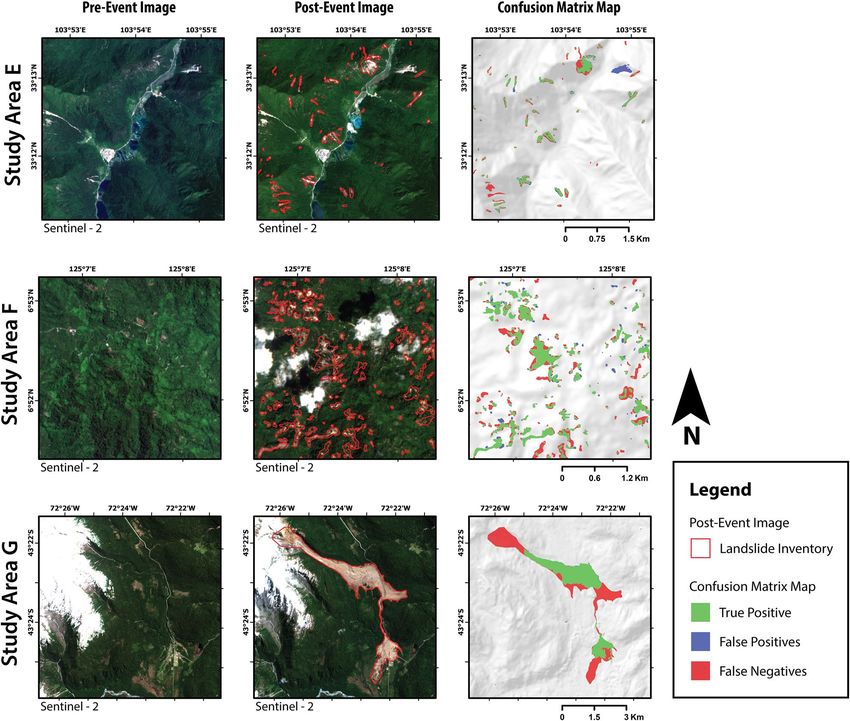
www.nature.com/scientificreports/
EO resources8. In this direction, the traditional pixel-based and object-based methods have been widely used
for mapping l andslides6, 9–11. Recent advances in deep learning have caused a paradigm shift in computer vision
algorithms used to extract information from i mages12–15. They are increasingly being adopted by the geosciences
community to find solutions for existing c hallenges16.
Many deep learning implementations to map landslides have been proposed in recent years, which typically
use a convolutional neural network (CNN) to learn directly from EO data17–21. These implementations have
outperformed traditional methods. Ghorbanzadeh et al.17 used RapidEye images combined with topographic
information derived from the 5 m ALOS digital elevation model (DEM) to train a CNN for detecting landslides.
Sameen and P radhan18 added residual connections in their network architecture to map landslides using aerial
images with topographic information from a lidar-derived DEM. The residual connections are identity mapping
functions that are used to construct alternate skip connections between the convolutional layers. Using residual
connections makes it easier for deep neural networks to optimize during the training process13. In these standard
CNN architectures, a series of convolutional layers/blocks are followed by fully-connected (FC) layers to predict
the output class labels. However, a U-Net replaces the FC layers with convolutional decoder blocks to output
a segmentation image14. Prakash et al.19 used a modified U-Net with ResNet34 backbone to perform semantic
segmentation of historic/old landslides from topographic features derived from LIDAR data. Different variants
of U-Net have also been used in multiple studies to map landslides from optical images in different geographical
regions22–24. These studies adopt a conventional supervised learning workflow where a model is first trained in
a controlled region (also known as the training region) and then reused to generate a landslide map of its sur-
roundings with comparable geo-environmental characteristics. In this approach, even the data source is often
not changed during the training and prediction processes. Models trained and validated using this approach
cannot be adopted for a fully autonomous pipeline that can rapidly map the new landslides after a post-event
image is acquired. However, deep learning architectures are known to generalize relatively well to unseen data
and therefore are often used in practice25,26. To truly harness the potential of deep learning, we need to change
our strategy from what has been used for traditional machine learning approaches.
In this work, we envision a scenario where a new landslide inventory is required immediately after a disaster
event that might have triggered multiple landslides over large areas. Machine learning algorithms trained and
validated using the existing approaches cannot be adopted for fully autonomous mapping of the new landslides.
Such approaches require a local landslide inventory created specifically for the event to train the deep learning
models. Depending on the geographic location and availability of resources, this inventory must be generated
using manual or semi-automated methods, which is a bottleneck for any rapid mapping a pplication4. To the
best of our knowledge, no study has yet explored the possibility of creating a generalized deep learning model
for mapping landslides beyond the spatial and temporal bounds of its training dataset.
Here, we propose a new combined training strategy to build a CNN-based semantic segmentation model gen-
eralized for identifying changes associated with landslide activity using a set of pre- and post-event EO images.
For this, we have used a deep network architecture, a large training dataset from multiple sensors and landslide
inventories, and strong data-augmentation to make the CNN learn features to map landslides generated by an
unseen/future triggering event. Multiple experiments have been designed to validate the proposed deep learn-
ing method in different operational scenarios. (I) The first set of experiments explores the potential of the deep
learning method. These experiments adopt a conventional approach to train a separate CNN model for each
area of interest. (II) The next set of experiments explores the idea of having a common CNN model trained on a
combined inventory from multiple study areas. (III) Lastly, the CNNs’ generalization ability is tested by apply-
ing them to new regions/triggers that were never encountered in the training process. In addition, because the
scale of analysis has always been crucial in landslide mapping algorithms, we also explore how the resolution of
inputs to the CNNs influences all three experiments.
In the following, the term ‘landslide event’ or “landslides” will always refer to a group of slope failure phe-
nomena generated by a single trigger, i.e., an earthquake or extreme rainfall events. The term ‘inventory’ will
refer to a catalogue of landslides induced by one trigger.
Study areas and dataset
We selected a total of seven study areas (identified by letters A to G), which experienced landslide events asso-
ciated to different triggers. We intentionally chose events after mid-2015 to exploit the data from Sentinel-2
images, which are available for free at a spatial resolution of 10 m. This ensured that the deep learning models
generated from this work could be easily adapted for mapping in new areas without being dependent on com-
mercial satellites. Figure 1 shows a geographic overview of the study areas along with additional information
on the trigger, spatial extent, and dataset used. Mapping landslides from optical data can be hindered by the
presence of clouds and thus can only be done in cloud-free regions. Depending on the local weather pattern, the
availability of cloud-free days can be scarce in the area of interest. There could be a delay in the order of months
to get an image of the affected region under clear skies. In this work, the satellite image tiles were selected with
a low cloud cover without increasing the temporal distance from the triggering event. The topographic infor-
mation for all the study areas was derived using the ALOS Global Digital Surface Model (AW3D30), which is
available at a resolution of 30 m.
Study area A (Myanmar). In 2015, the Ching State of Myanmar experienced Cyclone Komen in July,
along with unprecedented extreme rainfalls during the monsoon months. The Arakan mountain range covers a
significant portion of the Ching state with steep slopes and unstable geologic c onditions27. This led to widespread
flooding and landsliding, which caused extensive damage to infrastructure and loss of life. For this study area,
we selected an extent of 990 km2 in the north of Hakha city. The inventory from an existing work done by Alvioli
Scientific Reports | (2021) 11:9722 | https://doi.org/10.1038/s41598-021-89015-8 2
Vol:.(1234567890)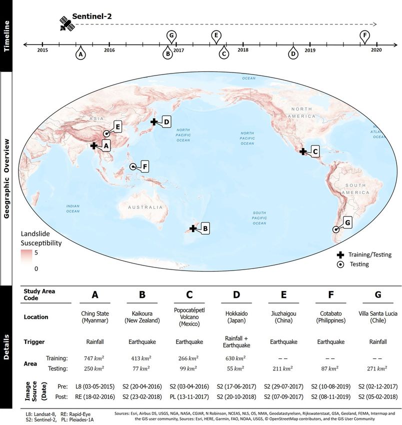
www.nature.com/scientificreports/
Figure 1. The map shows a geographic overview of the study areas over a background of global landslide
susceptibility51. They are located around the Pacific Ocean, which is a seismically active zone with a high
hydrological hazard d istribution52. The approximate date of occurrence for the events are marked on a timeline
(top). More details on the type of trigger, area of coverage, and optical data used for landslide mapping are
presented in the table (bottom). Only study areas A to D will be used for training the CNN models in this work.
The magnitude-frequency for all the landslide inventories is shown in Supplementary Figure 1. The map was
created using ArcGIS Pro v2.4 (https://www.esri.com/).
et al.28 was used to train the deep learning models. The authors have used pre- and post-event RapidEye images
to map 2131 event landslides, ranging from 162 m2 to 6.2 km2. Many large landslides were recorded in this area,
where the largest was the Tonzang landslide with a runout length of more than 5 km.
Study area B (New Zealand). The South Island of New Zealand experienced a Mw 7.8 earthquake on
14 November 2016, with its epicenter approximately 60 km south-west of Kaikoura. This event triggered more
than 10,000 landslides in sparsely populated regions, which fortunately resulted in no reported landslide-related
Scientific Reports | (2021) 11:9722 | https://doi.org/10.1038/s41598-021-89015-8 3
Vol.:(0123456789)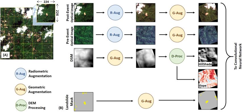
www.nature.com/scientificreports/
fatalities29. However, these landslides caused substantial damage to infrastructure and dammed rivers at multiple
locations. We selected a 490 km2 region between the earthquake epicenter and Kaikoura city as our study area.
Multiple works have been done for mapping the landslides triggered by the Kaikoura earthquake using high-
resolution images29,30. In this work, a new landslide inventory was created to train the deep learning models. A
total of 547 landslides were mapped with affected areas ranging from 112 m2 to 0.5 km2.
Study area C (Mexico). The Mw 7.1 Puebla earthquake, which occurred on 19 September 2017, caused
severe damage to life and property in Central Mexico. Coincidentally this earthquake happened exactly 32
years after the devastating Mexico City earthquake on 19 September 1985. Hundreds of shallow landslides were
triggered on the flanks of the Popocatepetl volcano, which is located approximately 70 km south-west of the
epicenter31. The study area selected for this event encloses the Popocatepetl volcano and has a total extent of
365 km2. In this work, a new landslide inventory was created to train the deep learning models. A total of 754
landslides were mapped with areas ranging from 216 m2 to 0.7 km2.
Study area D (Japan). The Mw 6.6 earthquake occurred in Hokkaido, Japan, on 6 September 2018. This
happened only a few days after this Northern island of Japan witnessed extensive rainfall due to Typhon Jebi.
The seismic shaking triggered an unusually high density (326 per km2) of co-seismic landsliding, which was
observed in an area of 700 km232. We considered this region as our study area, and the landslide inventory was
used from an earlier published w ork32. The authors manually mapped the co-seismic landslides using a set of
PlanetScope satellite images acquired on 11 September 2018. They were able to reject the non-coseismic land-
slides by manual cross-checking with pre-earthquake images collected on 22 March and 3 August 2018. The
inventory catalogs 7837 landslides with areas ranging from 74 m2 to 0.085 km2, which were used to train the
deep learning models.
Study area E (China). The Sichuan Province in China was struck by the Mw 6.5 Jiuzhaigou Earthquake on
8 August 2017. This induced many landslides in the form of small scale rockfalls and rock/debris slides33. For
this event, we selected a 200 km2 region as our study area. In this work, a new landslide inventory was created for
this study area for testing the deep learning models trained on other study areas. A total of 227 landslides were
mapped with affected areas ranging from 147 m2 to 0.1 km2.
Study area F (Philippines). The province of Cotabato in the Philippines was struck by a swarm of earth-
quakes in October 2019. Many of these events had a magnitude above Mw 5, with the highest magnitude reach-
ing Mw 6.6. These earthquake events triggered multiple landslides in two clusters. This is the most recent event
on our list, and it was difficult to find cloud-free images in Sentinel-2 and Google Earth Pro archives. For this
study, we carefully selected an 87 km2 study area to manually map the landslides in the southern cluster. This
inventory has 309 mapped landslides with affected areas ranging from 594 m2 to 0.19 km2 and will only be used
for testing the deep learning models trained on other areas.
Study area G (Chile). The southern Palena province of Los Lagos Region in Chile experienced torrential
rainfall on 15th and 16th of December 2017. This triggered a rockslide in the headwaters of Burrito River, which
was followed by large debris and mudflows that traveled for more than 8 km and caused heavy destruction in
ucia34. Unlike the previous study areas with hundreds of landslides, this study area in Chile has just
Villa Santa L
one large landslide, which impacted a total area of 7.73 km2. The deep learning models trained on other study
areas will be used to map the area affected by the Villa Santa Lucia landslide.
Results
We conducted experiments to train multiple CNNs on inventories from study areas A to D. For every training
scenario, we explored the influence of the base resolution on mapping performance. From here on, we follow a
naming convention to unequivocally identify an experiment, namely:
Trained CNN → MRSA
where, SA ∈ {A, B, C, D, ALL}
and, R ∈ {6 m, 10 m, 30 m}
Here, the super-script SA represents the Study Area used for training the CNN. When SA = ALL , the CNN
was trained on the combined inventories of study areas A to D. Similarly, the sub-script R represents the base
Resolution used for resampling the inputs to the CNN. For example, the symbol M10 A represents a CNN trained
on landslide inventory from study area A at a base resolution of 10 m.
Performance evaluation of conventional learning approach. We trained ten CNN models on each
inventory from study areas A to D at different base resolutions. In general, the CNNs were able to learn the
features required to map landslides in their respective testing regions. The dashed pink lines in Fig. 2 represent
the CNNs trained with a conventional learning approach. The best mapping performance was observed for M6A,
which got a Matthews Correlation Coefficient (MCC) score of 0.806. The models showed the weakest perfor-
mance in study area B, with the best MCC score of only 0.574 (by M10 B ). The best performance of study areas A,
C, and D was observed while mapping at a base resolution of 6 m. On the other hand, the best performance of
study area B was observed at a base resolution of 10 m. The CNN takes a tile of 224 × 224 pixels as input, which
Scientific Reports | (2021) 11:9722 | https://doi.org/10.1038/s41598-021-89015-8 4
Vol:.(1234567890)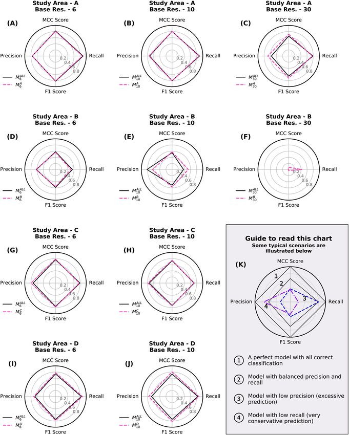
www.nature.com/scientificreports/

                                  Figure 2.  The spider plots (A–J) show the performance of CNNs trained with conventional learning (dashed
                                  line in pink) and combined learning (solid line in black) approaches. Every row has models evaluated for a
                                  specific study area at different base resolutions. The precision and recall scores are plotted on the X-axis, and the
                                  MCC and F1 scores are plotted on the Y-axis. (K) illustrates the shape expected from a good model which can
                                  be differentiated from models with lower precision or recall scores. The envelope of a better model will have a
                                  higher MCC/F1 Score and will enclose the plot from a weaker model. (Res. = Resolution).

Scientific Reports |   (2021) 11:9722 |                https://doi.org/10.1038/s41598-021-89015-8                                                    5

                                                                                                                                                Vol.:(0123456789)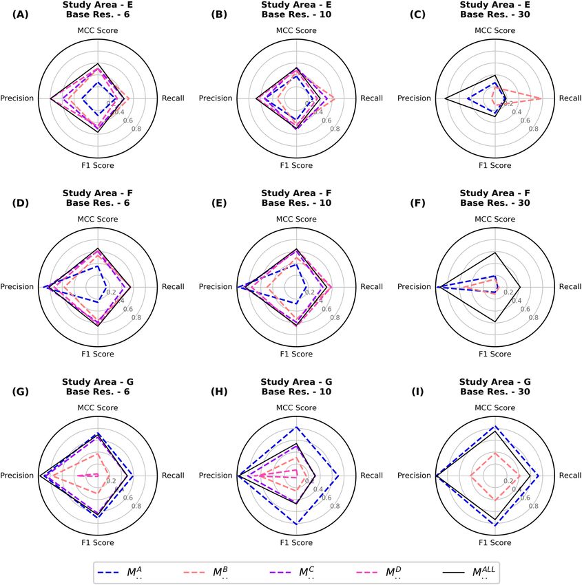
www.nature.com/scientificreports/
corresponds to a footprint of 1.34 × 1.34 km at a base resolution of 6 m. But when training is done at a base reso-
lution of 30 m, the footprint on the ground increases to 6.72 × 6.72 km. The testing regions identified in study
areas C and D were smaller than 6.72 km in at least one dimension (easting or northing). As a result, for these
two study areas, we were unable to use the CNNs for mapping at a base resolution of 30 m.
Performance evaluation of combined learning approach. We trained three CNN models on com-
bined inventories from study areas A to D at different base resolutions. The CNNs trained on combined invento-
ries performed similarly to those trained with a conventional approach (Fig. 2). Mapping landslides with M6ALL
in study area A resulted in the best reproduction of the ground truth, with an MCC score of 0.818. Even the
combined models showed the weakest performance scores in study area B, where M6ALL produced a maximum
MCC score of 0.58 across all the base resolutions. M30ALL failed map anything in this study area. In Fig. 3, we show
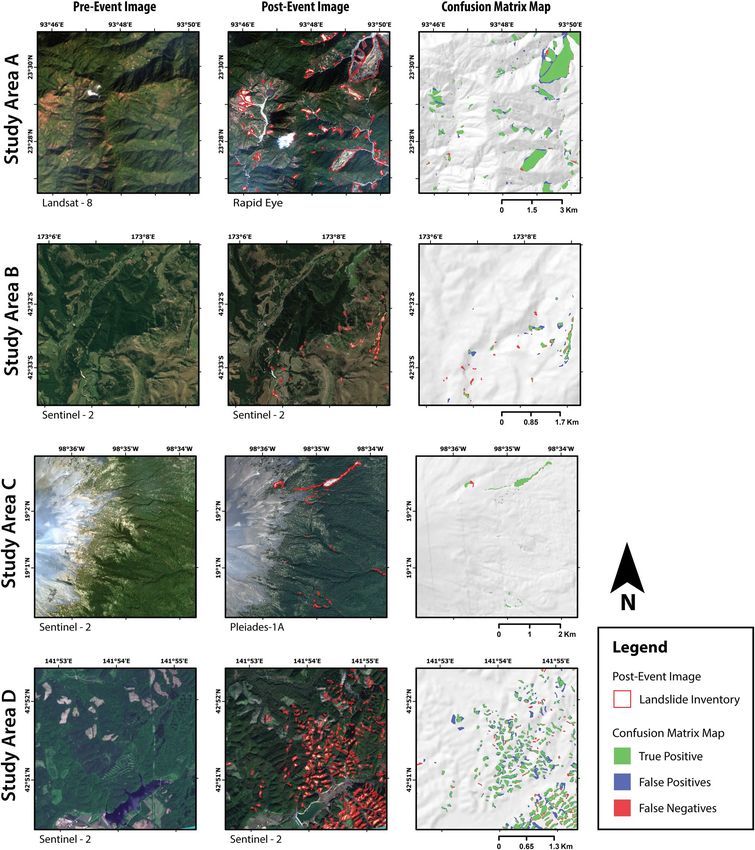
an example of the confusion matrix map generated by M6ALL for study area A to D to show the true positive (TP),
false positive (FP), and false negative (FN) predictions. The true negative (TN) predictions, which are the regions
correctly identified as “not-landslide” by the CNNs, are not shown on the map as a separate label.
Generalization performance. To test the generalization performance, the CNNs trained in the above
experiments were used to map landslides in a new geo-environmental setting, i.e., without using a local training
inventory. Figure 4 compares the performance of all the trained CNNs for mapping landslides in study area E
to G. The model M6ALL showed the best performance scores for study areas E and F, with an MCC score of 0.59
and 0.65 respectively. In study area G, the best performance was observed by M30 A with an MCC score of 0.842,
which was closely followed by M10. We observed the mapping of the CNNs on unseen regions is biased towards
A
high precision with relatively low recall. This means that the area identified as a landslide can be trusted with
high confidence, but the inventory is not complete as it also misses out on many landslides. For study area G, the
highest recorded precision score was 0.991 and while the recorded highest recall scores were only 0.727 (both for
M30A ). Figure 5 shows an example of the confusion matrix map generated by M ALL for study area E to G.
..
Discussions
CNNs are widely used for automatic interpretation of satellite images to retrieve valuable information. The pro-
posed method performed well for mapping event landslides in their corresponding testing regions. Figure 3K is
a guide for interpreting the behavior of the CNNs, which have been visualized on the spider plot. A model with
a perfect correspondence to the ground truth will have a value of 1 for MCC, F1, precision, and recall scores.
However, it is difficult to accurately delineate the precise boundary of most landslides in the real world. It is com-
mon for experts to disagree and have conflicting interpretations of the spatial extent of landslides present in any
specific area35. We do not expect the landslide map generated by a CNN to be exactly equal to the ground truth
inventory. A good performing CNN is indicated by a high MCC score with balanced precision and recall scores.
A CNN biased towards low recall and high precision scores will be very conservative in mapping and overlook
many landslides affected areas. On the other hand, a CNN with high recall and low precision scores will be very
aggressive in mapping by overpredicting many stable slopes as landslides. A model biased towards higher recall
values would be generally preferred for an inventory mapping done for risk assessment and disaster management.
In this work, we continuously tracked the consequence of changing the resolution of the input data. Any
changes to the base resolution will directly influence the extent of spatial context observed by the CNN in one
pass. A tile with a base resolution of 6 m corresponds to a ground footprint of 1.34 × 1.34 km (1.8 km2 ), whereas
a tile with a base resolution of 30 m will correspond to a ground area of 6.72 × 6.72 km (45.1 km2 ). Thus, the tile
with a smaller base resolution might not see the full extent of a large landslide. This can justify the performance
of CNNs tested at a base resolution of 30 m in study areas A and G, as both have large landslides triggered by
extreme rainfall. However, a tile with a higher base resolution can distinguish finer surface features, essential
for identifying landslide affected areas.
In our study, we found the conventional and combined learning models to have a small bias towards higher
recall scores when tested on study areas A to D (Fig. 3A–J). The best MCC scores for these study areas were
above 0.7, except for study area B. The low scores were caused by many small landslides in the testing region of
study area B, which were completely missed by the CNN. All the models in the training study areas showed the
weakest performance at a base resolution of 30 m . We also observe that CNNs trained at a base resolution of
6 m always achieve a higher MCC score than similar models at a base resolution of 10 m. The performance gain
between the two base resolutions is not very significant, with improvements ranging from a margin of 0.003 to
0.03. Here, M10 A (MCC score: 0.560) is an exception which was outperformed by M B (MCC score: 0.574). We
10
have used data from high-resolution satellites for the post-event image in study areas A and C (Rapid-eye and
Pleiades, respectively). This was done for two reasons: (i) these images from the commercial satellites was avail-
able to us, and (ii) we were able to test our method on other medium resolution images apart from Sentinel-2.
This higher resolution of inputs could partially explain the marginally higher MCC scores for models trained
at a base resolution of 6 m in study areas A and C. However, the same advantage is not applicable for study area
D, which also shows a similar trend in MCC scores while using Sentinel-2 images. Using images sampled at a
higher resolution of 6 m, we generate more tiles for the same extent of a study area, thereby virtually increasing
the number of images available for training. A similar practice of upsampling images to achieve better results
exists in other satellite image processing applications like image co-registration36.
Unlike what we observe in study areas A to D, we notice that the combined learning method has an advantage
in mapping landslides in a new area (Fig. 5). For study areas E and F, the combined learning CNNs consistently
performed better than their conventional learning counterparts, with the best results coming from M6ALL . The
landslides in these two study areas are triggered by earthquakes. This might also explain why conventional
Scientific Reports | (2021) 11:9722 | https://doi.org/10.1038/s41598-021-89015-8 6
Vol:.(1234567890)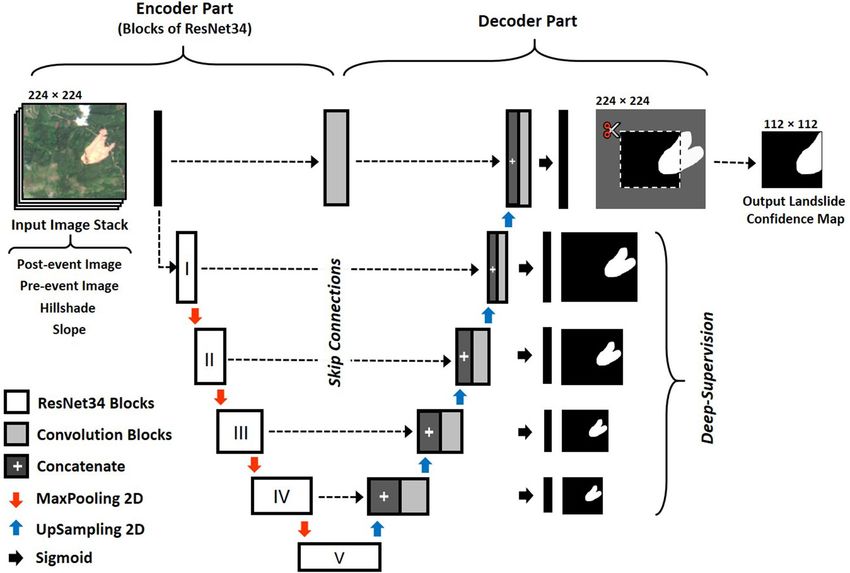
www.nature.com/scientificreports/
Figure 3. Result of applying the trained CNN model ( M6ALL) on the testing region of study area “A” to “D”.
Every row shows a fixed view from one study area with pre-event image (left), post-event image with polygons
from landslide inventory (middle), and output from CNN as a confusion matrix map (right). The majority
resampling method was used to visualize the confusion matrix map. The cloud and snow-cover masks have not
been shown for clarity, but the affected region was not used in the training and prediction process. The maps
were created using ArcGIS Pro v2.4 (https://www.esri.com/).
learning CNNs’ performance in study areas B to D (also earthquake-triggered) is also not very low. However, the
same models showed a poor performance while mapping the rainfall triggered Santa Lucia landslide in study area
G. M10
A and M A had the best performance while mapping this large landslide, closely followed by the combined
30
Scientific Reports | (2021) 11:9722 | https://doi.org/10.1038/s41598-021-89015-8 7
Vol.:(0123456789)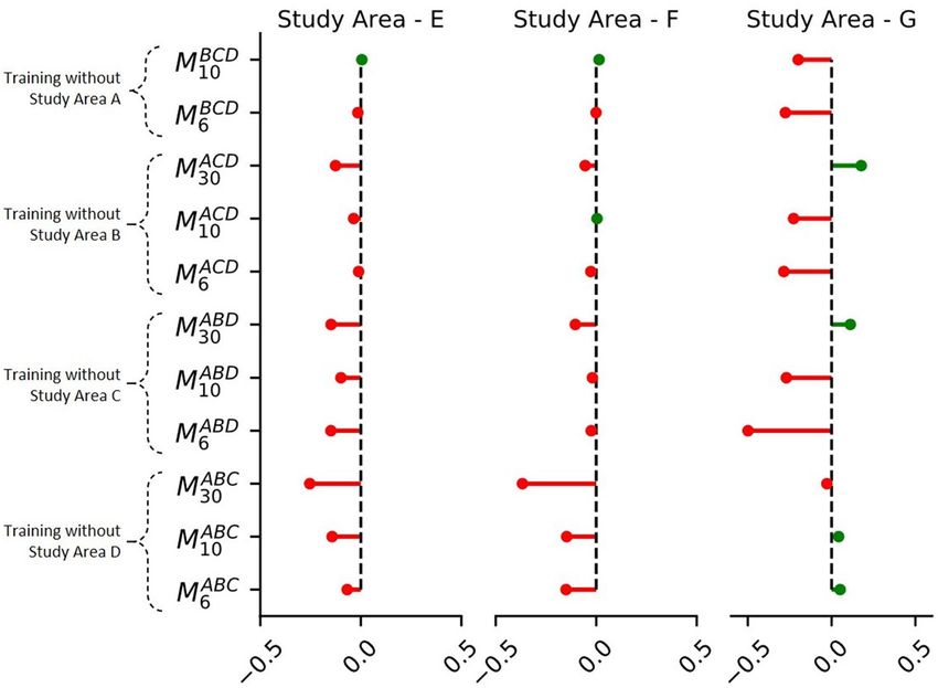
www.nature.com/scientificreports/
Figure 4. The plots (A–I) compare the generalization of conventional learning and combined learning models.
Every row evaluates landslide mapping performance for unseen events in the study area “E” to “G”. The guide to
read this plot is illustrated in Fig. 2 (K). (Res. = Resolution).
learning model M30 ALL . An explanation for the poor performance of M ALL in study area G can be explained by
..
the under-representation of rainfall triggered landslide inventories in the training data.
We found that the CNNs performance on new areas was biased towards higher precision scores. This is simi-
lar to observations from other deep learning work done in the area of domain generalization and multidomain
learning37. To rule out any negative contributions from any of the four training inventories used by the combined
learning models, we adopted a jackknife approach by conducting more experiments to train CNNs from only
three study areas, while systematically leaving out one each time. Figure 6 shows the changes in MCC scores for
these new CNNs as compared to the scores for M6ALL. We found that training without rainfall triggered inventory
from study area A improves the MCC score in earthquake-affected study areas E and F. But, it also decreases the
MCC score for the rainfall-affected study area G. No single inventory removal contributed to an overall improve-
ment in the performance of the combined model. Thus, future efforts should instead be focused on expanding
the training dataset by progressively adding new inventories from more landslide events.
Scientific Reports | (2021) 11:9722 | https://doi.org/10.1038/s41598-021-89015-8 8
Vol:.(1234567890)www.nature.com/scientificreports/
Figure 5. Result of applying the trained CNN model ( M6ALL) on study area “E” to “G”. These three study areas
were not used for training any CNN model; hence they were completely used as the testing region. The results
highlight the generalizing ability of M6ALL to map event landslides. Every row shows a fixed view from one
study area with pre-event image (left), post-event image with polygons from landslide inventory (middle), and
output from CNN as a confusion matrix map (right). The majority resampling method was used to visualize the
confusion matrix map. The cloud and snow-cover masks have not been shown for clarity, but the affected region
was not used in the training and prediction process. The maps were created using ArcGIS Pro v2.4 (https://www.
esri.com/).
The FP and FN detections in the confusion matrix maps are often observed on the boundaries of the ground
truth inventories, or due to amalgamation of closely located landslides (Figs. 2 and 4). The FP detections should
not be overlooked as they could also point to a new landslide that is missing in the ground truth inventory. As
discussed in the above paragraph, the performance of CNNs on study area E to G is biased towards high preci-
sion and low recall scores. This can be observed in the confusion matrix maps of Fig. 4, where significant FN
detections completely miss out on many landslides. This does not necessarily mean a bad result, as we are still
correctly mapping many landslides with high precision without specifically training a new CNN on that particular
area. To understand the current situation from a recent event, we can look at the timeline of image acquisition
and mapping effort compiled by William et al.4 after Mw 7.8 Gorkha earthquake of 25th April 2015. The first two
maps were created after one week, which identified less than 500 landslides as point features. It took many weeks
to generate a more detailed inventory with 5600 landslides delineated as polylines. For the same disaster, the
number of landslides identified grew by a factor of five after a few years of mapping e fforts3. An algorithm that
can rapidly generate a first cut map of areas affected by landsliding after a disaster would be valuable for plan-
ing any relief operations. Once more time is available, the affected area can be remapped with the conventional
approach using the trained CNN as a pre-trained model for an updated landslide map with higher accuracy.
Scientific Reports | (2021) 11:9722 | https://doi.org/10.1038/s41598-021-89015-8 9
Vol.:(0123456789)www.nature.com/scientificreports/
Figure 6. Jackknife’s approach for training new CNNs on combined landslide inventories. Here, we rule out the
possibility of a bad inventory bringing down the performance of the combined learning approach. The values
in X-axis are the difference of MCC score of the new model with the MCC score of M6ALL. A red line shows a
decrease in MCC score, and a green line shows an increase in MCC score. An example of nomenclature used
here: the symbol M6ABC represents a new combined learning model which has been trained on study area A, B,
and C at a base resolution of 10 m.
However, this method does not work if the pre- or post-event optical image has been affected by cloud or
snow. The pre-event image used in study area G was covered in snow, resulting in an FN detection in the head
scarp region of the Santa Lucia landslide (Fig. 4). This could be a serious problem for some cases as it might take
many days for the clouds to clear the sky. Methods working on spaceborne Synthetic Aperture Radar data can
provide information even through cloud cover and should be used for such situations38,39. All the study areas
selected for this study had had high coverage of vegetation. In future works, landslides and EO data from less
vegetated geographic locations should be included in the training and testing datasets. Deep learning models are
very good at learning from the training dataset. The algorithm also learns the biases of the expert who is map-
ping landslides for the training process. Hence, high quality of correctness should be ensured for the landslide
inventory used for training the model. Using a large dataset of many inventories generated by multiple experts
is expected to decrease this problem.
Conclusions
Automated mapping of landslides is a challenging task. Experts commonly use a set of pre- and post-event images
to delineate landslides using manual or semi-automated methods. This study proposed a new strategy for training
a deep learning model to map event landslides from medium resolution EO data. Seven post-2015 triggers in
different tectonic settings were selected for training and testing the CNN models. New landslide inventories were
prepared for four triggers for which public records were not available or were unsuitable for this work. The CNNs
were trained separately on four inventories using a conventional supervised learning approach. The performance
scores of the trained models were evaluated by applying them to the hold-out regions of their respective study
areas. However, a CNN trained using a conventional approach is not expected to map landslides induced by a
different trigger from another geographic location.
The lack of training data is a common problem in the effective deployment of a data-driven model for a near
real-time landslide mapping task. This study addresses the issue by testing the generalization performance of
CNNs to map landslides induced by three triggers that were not seen by the CNN during the training process.
Results show that a CNN trained on a combination of landslide inventories from multiple triggers has a better
generalization than a similar CNN trained with a conventional approach. We also observed that mapping the
landslides induced by new and unseen triggers is biased towards high precision and low recall scores. However,
this is not an issue as such CNNs can be used on future triggers in new geo-environmental settings without a re-
training step. We also provide access to a pre-trained model and a Jupyter Notebook script, making it convenient
to map an event landslide inventory in a new area of interest.
Scientific Reports | (2021) 11:9722 | https://doi.org/10.1038/s41598-021-89015-8 10
Vol:.(1234567890)www.nature.com/scientificreports/
Figure 7. Pre-processing workflow adopted for training of CNN. (A) Systematic tiling of input images with
50% overlap. In this study , a tile size of 224 × 224 was used as an input to the CNN. The tile size in display is
for representation purposes and does not scale to the actual base resolution used in training the CNN. (B) Steps
involved in the data-augmentation of input images with their corresponding landslide mask.
Methods
In this study, a modified U-Net architecture was used for the automatic semantic segmentation of landslide
events. We train the CNN models on landslide inventories from study areas A to D. Hence, the extent of these
four study areas is further sub-divided into non-overlapping training and testing regions. The holdout testing
region is used for evaluating the performance of the trained models. On the other hand, we do not use study
areas E to G in the training process. The full extent of these study areas is used as a testing area for evaluating
the trained models’ generalizing ability. The next sub-sections give a detailed description of the procedure we
followed to map and evaluate the landslide inventory.
Visual interpretation of landslides. The landslide inventories are prepared by visually identifying
regions affected by the landslide event. A set of pre- and post-event true color composites of Sentinel-2 images
along with corresponding AW3D30 digital surface model were used to delineate landslides as a vector polygon.
However, as an exception, we used high-resolution Pleiades-1A image acquired on 13 November 2017 for map-
ping landslides triggered by the Puebla earthquake (study area C).
Mapping landslides from medium resolution satellite images is a challenging task. The optical images were
draped over a 3D terrain model to get a better visualization of the topography during the mapping process.
High-resolution multi-temporal images available in Google Earth Pro software package were used for identify-
ing very small landslides and doubtful cases. We often noticed minor registration issues when comparing data
from multiple sources. As a result, a mapped landslide polygon from one image source appeared with a minor
shift on a different image source, especially on some high-resolution Google Earth images. To keep a consistent
mapping scheme, the final landslide polygons were created to mark the landslide extent visible on post-event
images mentioned in Fig. 1.
It should be noted that the inventory of event-triggered landslides was generated for a limited scope of train-
ing a CNN for a segmentation task and lacks any information on the type of movement, volume of the landslide,
or its forming material.
Preprocessing and data augmentation. The first step of preprocessing involved masking out the clouds,
shadows, and snow present in the pre- and post-optical images. This mask was created manually for this study,
but any automated algorithm can be used for this t ask40,41. All the input data sources were available at different
resolutions and had to be resampled to a common base resolution. The dimensions of EO images are generally
very large and cannot be used directly as an input to a CNN. To overcome this problem, it has been a common
practice to divide the image into smaller and manageable image patches called tiles. In this study, we systemati-
cally extracted tiles of 224 × 224 pixels from the set of input images (Fig. 7A). While extracting the tiles for the
training process, an overlap factor of 50% was used to increase the number of samples available for training the
network. The corresponding binary landslide masks were generated by rasterizing the available inventory at the
desired base resolution.
The training of CNN requires a large number of labeled images. Also, a typical CNN has millions of trainable
parameters, making it very efficient in learning the perfect parameters to over-fit the training data42. This limits
Scientific Reports | (2021) 11:9722 | https://doi.org/10.1038/s41598-021-89015-8 11
Vol.:(0123456789)www.nature.com/scientificreports/
the generalization ability of the trained model. Data augmentation is a commonly adopted practice in deep-
learning to artificially increase the sample count of the training dataset by applying valid random transformations.
It also increases the diversity of the training dataset, which helps in regularizing the trained model to improve
generalization42,43. We applied strong augmentations to the set of input images and landslide masks (Fig. 7B).
These augmentations can be broadly categorized into radiometric augmentation (R-Aug) and geometric augmen-
tation (G-Aug). R-Aug includes transformation functions to make random changes in the appearance of images,
which include changes in colors, blurring/sharpening, and addition of noise. On the other hand, G-Aug includes
transformation functions to alter the geometry of images with random flipping and affine transformations. The
state of randomness in R-Aug is different when it is applied to a set of pre- and post-optical images. But the
state of randomness in G-Aug is kept constant when it is applied to a set of input images and its corresponding
landslide mask. This makes intuitive sense as the pre- and post-images can have some differences in noise and
colors. However, if one image from a set is perturbed with geometric transformations like a rotation of +20°, all
the other images must be rotated by the same amount to have a coherent set of images. Finally, hillshade and
slope maps were generated after G-Aug has been applied to the DEM. The topographic information will help in
reducing FP detection in flat regions. The stack of these augmented topographic and optical images paired with
the corresponding augmented landslide mask is used to train the CNN.
There are many earth observation satellites in operation. It is possible to observe a landslide event using
multiple combinations of pre- and post-event data by varying the source of satellites image and their date of
acquisition. In the conventional approach adopted in previous studies, the set of data used during prediction and
training is the same. However, a generalized CNN is expected to map landslides from any optical data source.
Therefore, it is also possible to increase the number of images available for training by adding more combinations
of pre- and post-event images. For training the combined learning models in study areas A and C, we supplement
the high-resolution dataset with an extra set of Sentinel-2 image pairs.
Convolutional neural network. U-Net has been introduced by Ronneberger et al.14 for segmentation of
biomedical images and has been adopted for many different a pplications19,44. A U-Net is a fully-convolutional
CNN that consists of a downsampling part that acts as an encoder. Skip connections from the encoder part
to the decoder part help the CNN recover its full spatial r esolution45. In this work, we use a modified U-Net,
which was made deeper by replacing the convolutional blocks with blocks of residual network with identity
mappings (Fig. 8). These residual networks enable the training of deeper models without degrading the network
performance13. Dropout layers and L2 regularization were used to increase the CNN’s generalization ability. In
addition, the U-Net was also deeply supervised at all the blocks in the upsampling p art15.
In the proposed architecture, ReLU was used as the activation function after every convolution operation.
The final prediction layer is generated after a 1 × 1 convolution with sigmoid activation. This generates an output
image with confidence values ranging from 0 to 1, which is thresholded at 0.5 to get a binary segmentation mask.
During prediction, an overlap-tile strategy was applied by selecting the center 112 × 112 pixels of the output
image for generating a seamless segmentation map of very large images14,19.
Training process. The entire process is implemented in Python using GDAL46 for GIS processing, Keras47
and TensorFlow48 for machine learning. Before the start of training, a small section of the training area was kept
aside for validation.
We used a combination of focal Tversky index (FTI) and binary cross-entropy (BCE) as a loss function dur-
ing the training process19,49. The total loss (L ) is a weighted sum of the loss from the deeply supervised layers
(L i , i = 1, 2, 3, 4) and the final output layer (L 0 ).
4
L = wi L i
i=0
The value of hyper-parameter w0 = 5 and w1−4 = 1. Also, L i is given by:
L i = 0.2 × LBCE
i i
+ 0.8 × LFTI
Adam optimizer was used to minimize the total loss (L ) with a learning rate of 10−4. After every epoch of train-
ing, the validation loss (total loss in the held-out validation set) was evaluated. The learning rate was decreased
by 0.1 if the validation loss plateaued or started rising for three continuous epochs. The training process was
stopped if there was no further drop in validation loss was recorded for ten continuous epochs. The model with
the lowest validation loss during the training process was used to map landslides in testing regions.
Performance evaluation. CNN’s performance was evaluated by applying the trained model to the holdout
testing areas. The landslide inventories used in this work served as the ground truth labels. The binary map of
predicted landslides was compared with the ground truth to generate a map of confusion matrix values (for e.g.,
Figs. 2 and 4), i.e., TP, FP, FN, and TN values. Here, TP represents the correctly predicted landslides, and TN
represents correctly identified regions with no landslide activity. The FP represents the landslides predicted by
the CNN, which is missing in the ground truth. Similarly, the FN represents the landslides that the CNN has
missed. In the next steps, these confusion matrix values were used to calculate few commonly used metrics for
the statistical analysis of the binary classification. Ideally, in machine learning, the accuracy score is considered a
reliable metric for evaluating a trained model’s performance. However, landslide classification is a highly unbal-
anced learning task where the spatial extent of the landslide affected area is much smaller than the stable areas.
Scientific Reports | (2021) 11:9722 | https://doi.org/10.1038/s41598-021-89015-8 12
Vol:.(1234567890)www.nature.com/scientificreports/
Figure 8. An overview of proposed U-Net architecture with residual blocks and deep-supervision. The
complete description of all the layers in the network is available in Supplementary Figure 2.
Metric Formula
F1-score 2TP
2TP+FP+FN
MCC √ TP×TN−FP×FN
(TP×FP)(TP×FN)(TN×FP)(TN×FN)
Precision TP
TP+FP
Recall TP
TP+FN
Table 1. Derivation of performance evaluation metrics from confusion matrix values.
As a result, the accuracy score becomes unreliable due to very high true negative values. This study reports the
F1-Score, MCC score, precision, and recall values plotted in a spider chart (Table 1). We consider the MCC score
to be the most suitable metric for comparing and ranking the CNN models tested in this work50. Understand-
ing an MCC score is also intuitive for a binary classifier, with 0 indicating a model with no correlation (random
guesses) and 1 indicating a perfect correlation (all correct guesses).
Data availability
The weights and network architecture of CNN model trained using the combined learning approach is publicly
available at https://g ithub.c om/n
prksh/l andsl ide-m
appin
g-w
ith-c nn. The repository also contains a Jupyter Note-
book, which explains the steps required for mapping landslides in a new area of interest. The inputs required are
a DSM and a pair of pre- and post-event Sentinel-2 images. This Notebook can be further forked/modified to
map landslides in any other area of interest or with a set of true-color composites from a different sensor. In the
same repository, we also deliver four new event-landslide inventories (study areas B, C, E, and F), which were
created as a part of this study. The datasets can be used in future studies for the analysis of specific events, as well
as in the development of new machine learning methods.
Received: 23 November 2020; Accepted: 20 April 2021
Scientific Reports | (2021) 11:9722 | https://doi.org/10.1038/s41598-021-89015-8 13
Vol.:(0123456789)www.nature.com/scientificreports/
References
1. Turner, A. K. Social and environmental impacts of landslides. Innov. Infrastructure Solut. 3, 70. https://doi.org/10.1007/s41062-
018-0175-y (2018).
2. Froude, M. J. & Petley, D. N. Global fatal landslide occurrence from 2004 to 2016. Nat. Hazards Earth Syst. Sci. 18, 2161–2181.
https://doi.org/10.5194/nhess-18-2161-2018 (2018).
3. Roback, K. et al. The size, distribution, and mobility of landslides caused by the 2015 mw7.8 gorkha earthquake, Nepal. Geomor-
phology 301, 121–138. https://doi.org/10.1016/j.geomorph.2017.01.030 (2018).
4. Williams, J. G. et al. Satellite-based emergency mapping using optical imagery: Experience and reflections from the 2015 Nepal
earthquakes. Nat. Hazards Earth Syst. Sci. 18, 185–205. https://doi.org/10.5194/nhess-18-185-2018 (2018).
5. Galli, M., Ardizzone, F., Cardinali, M., Guzzetti, F. & Reichenbach, P. Comparing landslide inventory maps. Geomorphology 94,
268–289. https://doi.org/10.1016/j.geomorph.2006.09.023 (2008).
6. Tanyaş, H. et al. Presentation and analysis of a worldwide database of earthquake-induced landslide inventories. J. Geophys. Res.
Earth Surf. 122, 1991–2015. https://doi.org/10.1002/2017jf004236 (2017).
7. Guzzetti, F. et al. Landslide inventory maps: New tools for an old problem. Earth Sci. Rev. 112, 42–66. https://doi.org/10.1016/j.
earscirev.2012.02.001 (2012).
8. Dlr—earth observation center—60 petabytes for the German satellite data archive d-sda. https://www.dlr.de/eoc/en/desktopdef
ault.aspx/tabid-12632/22039_read-51751. Accessed 13 July 2020.
9. Stumpf, A. & Kerle, N. Object-oriented mapping of landslides using random forests. Remote Sens. Environ. 115, 2564–2577. https://
doi.org/10.1016/j.rse.2011.05.013 (2011).
10. Alvioli, M. et al. Automatic delineation of geomorphological slope units with r.slopeunits v1.0 and their optimization
for landslide susceptibility modeling. Geosci. Model Dev. 9, 3975–3991. https://doi.org/10.5194/gmd-9-3975-2016 (2016).
11. Mondini, A. et al. Semi-automatic recognition and mapping of rainfall induced shallow landslides using optical satellite images.
Remote Sens. Environ. 115, 1743–1757. https://doi.org/10.1016/j.rse.2011.03.006 (2011).
12. Krizhevsky, A., Sutskever, I. & Hinton, G. E. ImageNet classification with deep convolutional neural networks. Commun. ACM
60, 84–90. https://doi.org/10.1145/3065386 (2017).
13. He, K., Zhang, X., Ren, S. & Sun, J. Deep residual learning for image recognition. CoRRarxiv:abs/1512.03385 (2015).
14. Ronneberger, O., Fischer, P. & Brox, T. U-net: Convolutional networks for biomedical image segmentation. CoRRarxiv:abs/1505.
04597 (2015).
15. Wang, L., Lee, C., Tu, Z. & Lazebnik, S. Training deeper convolutional networks with deep supervision. CoRRarxiv:abs/1 505.0 2496
(2015).
16. Zhu, X. X. et al. Deep learning in remote sensing: A comprehensive review and list of resources. IEEE Geosci. Remote Sens. Mag.
5, 8–36. https://doi.org/10.1109/mgrs.2017.2762307 (2017).
17. Ghorbanzadeh, O. et al. Evaluation of different machine learning methods and deep-learning convolutional neural networks for
landslide detection. Remote Sens. 11, 196. https://doi.org/10.3390/rs11020196 (2019).
18. Sameen, M. I. & Pradhan, B. Landslide detection using residual networks and the fusion of spectral and topographic information.
IEEE Access 7, 114363–114373. https://doi.org/10.1109/access.2019.2935761 (2019).
19. Prakash, N., Manconi, A. & Loew, S. Mapping landslides on eo data: Performance of deep learning models vs. traditional machine
learning models. Remote Sens. 12, 346. https://doi.org/10.3390/rs12030346 (2020).
20. Meena, S. R. et al. Rapid mapping of landslides in the western ghats (India) triggered by 2018 extreme monsoon rainfall using a
deep learning approach. Landslideshttps://doi.org/10.1007/s10346-020-01602-4 (2021).
21. Catani, F. Landslide detection by deep learning of non-nadiral and crowdsourced optical images. Landslides 18, 1025–1044. https://
doi.org/10.1007/s10346-020-01513-4 (2020).
22. Liu, P., Wei, Y., Wang, Q., Chen, Y. & Xie, J. Research on post-earthquake landslide extraction algorithm based on improved u-net
model. Remote Sens. 12, 894. https://doi.org/10.3390/rs12050894 (2020).
23. Qi, W., Wei, M., Yang, W., Xu, C. & Ma, C. Automatic mapping of landslides by the ResU-net. Remote Sens. 12, 2487. https://doi.
org/10.3390/rs12152487 (2020).
24. Yi, Y. & Zhang, W. A new deep-learning-based approach for earthquake-triggered landslide detection from single-temporal
RapidEye satellite imagery. IEEE J. Sel. Top. Appl. Earth Observ Remote Sens. 13, 6166–6176. https://doi.org/10.1109/jstars.2020.
3028855 (2020).
25. Dinh, L., Pascanu, R., Bengio, S. & Bengio, Y. Sharp minima can generalize for deep nets (2017). arxiv:1703.04933.
26. Kawaguchi, K., Kaelbling, L. P. & Bengio, Y. Generalization in deep learning (2020). arxiv:1710.05468.
27. Mon, M. M. et al. Analysis of disaster response during landslide disaster in Hakha, Chin State of Myanmar. J. Disaster Res. 13,
99–115. https://doi.org/10.20965/jdr.2018.p0099 (2018).
28. Mondini, A. Measures of spatial autocorrelation changes in multitemporal SAR images for event landslides detection. Remote
Sens. 9, 554. https://doi.org/10.3390/rs9060554 (2017).
29. Massey, C. et al. Landslides triggered by the 14 November 2016 Mw 7.8 Kaikōura earthquake, New Zealand. Bull. Seismol. Soc.
Am. 108, 1630–1648. https://doi.org/10.1785/0120170305 (2018).
30. Rathje, E., Little, M., Massey, C. & Wartman, J. Kaikoura Earthquake Landslide Inventoryhttps://doi.o S2508 W (2017).
rg/1 0.1 7603/D
31. Coviello, V. et al. Earthquake-induced debris flows at popocatépetl volcano, mexico. Earth Surf. Dyn. Discuss. 2020, 1–24. https://
doi.org/10.5194/esurf-2020-36 (2020).
32. Wang, F. et al. Coseismic landslides triggered by the 2018 Hokkaido, Japan (mw 6.6), earthquake: Spatial distribution, controlling
factors, and possible failure mechanism. Landslides 16, 1551–1566. https://doi.org/10.1007/s10346-019-01187-7 (2019).
33. Fan, X. et al. Coseismic landslides triggered by the 8th august 2017 ms 7.0 jiuzhaigou earthquake (Sichuan, China): Factors con-
trolling their spatial distribution and implications for the seismogenic blind fault identification. Landslides 15, 967–983. https://
doi.org/10.1007/s10346-018-0960-x (2018).
34. Duhart, P. et al. Santa lucía landslide disaster, chaitén-chile, the: origin and effects. In Kean, J. W., Coe, J. A., Santi, P. M. & Guillen,
B. K. (eds.) Debris-flow hazards mitigation: mechanics, monitoring, modeling, and assessment. In Proceedings of the 7th Interna-
tional Conference on Debris Flow Hazards Mitigation, Association of Environmental & Engineering Geologists Special Publication
Vol. 28, 653–660, https://doi.org/10.25676/11124/173159(2019).
35. Fan, X. et al. Earthquake-induced chains of geologic hazards: Patterns, mechanisms, and impacts. Rev. Geophys. 57, 421–503.
https://doi.org/10.1029/2018rg000626 (2019).
36. Xiong, Z. & Zhang, Y. A critical review of image registration methods. Int. J. Image Data Fusion 1, 137–158. https://doi.org/10.
1080/19479831003802790 (2010).
37. Bickel, V. T. et al. Deep learning-driven detection and mapping of rockfalls on mars. IEEE J. Sel. Top. Appl. Earth Observ Remote
Sens. 13, 2831–2841 (2020).
38. Esposito, G. et al. A spaceborne sar-based procedure to support the detection of landslides. Nat. Hazards Earth Syst. Sci. 20,
2379–2395. https://doi.org/10.5194/nhess-20-2379-2020 (2020).
39. Mondini, A. et al. Sentinel-1 SAR amplitude imagery for rapid landslide detection. Remote Sens. 11, 760. https://doi.org/10.3390/
rs11070760 (2019).
Scientific Reports | (2021) 11:9722 | https://doi.org/10.1038/s41598-021-89015-8 14
Vol:.(1234567890)www.nature.com/scientificreports/
40. Qiu, S., Zhu, Z. & He, B. Fmask 4.0: Improved cloud and cloud shadow detection in landsats 4–8 and sentinel-2 imagery. Remote
Sens. Environ. 231, 111205. https://doi.org/10.1016/j.rse.2019.05.024 (2019).
41. Hagolle, O., Huc, M., David, V. P. & Dedieu, G. A multi-temporal method for cloud detection, applied to FORMOSAT-2, VEN µ S,
LANDSAT and SENTINEL-2 images. Remote Sens. Environ. 114, 1747–1755. https://doi.org/10.1016/j.rse.2010.03.002 (2010).
42. Shorten, C. & Khoshgoftaar, T. M. A survey on image data augmentation for deep learning. J. Big. Data 6, 1–48. https://doi.org/
10.1186/s40537-019-0197-0 (2019).
43. Kukačka, J., Golkov, V. & Cremers, D. Regularization for deep learning: A taxonomy (2017). arxiv:1710.10686.
44. Peng, D., Zhang, Y. & Guan, H. End-to-end change detection for high resolution satellite images using improved unet++. Remote
Sens. 11, 1382. https://doi.org/10.3390/rs11111382 (2019).
45. Zhou, Z., Siddiquee, M. M. R., Tajbakhsh, N. & Liang, J. Unet++: A nested u-net architecture for medical image segmentation.
CoRRarxiv:abs/1807.10165 (2018).
46. GDAL/OGR contributors. GDAL/OGR Geospatial Data Abstraction software Library. Open Source Geospatial Foundation (2020).
47. Chollet, F. et al. Keras. https://keras.io (2015).
48. Abadi, M. et al. TensorFlow: Large-scale machine learning on heterogeneous systems (2015). Software available from tensorflow.
org.
49. Abraham, N. & Khan, N. M. A novel focal tversky loss function with improved attention u-net for lesion segmentation. CoRRarxiv:
abs/1810.07842 (2018).
50. Luque, A., Carrasco, A., Martín, A. & de las Heras, A. The impact of class imbalance in classification performance metrics based
on the binary confusion matrix. Pattern Recogn. 91, 216–231. https://doi.org/10.1016/j.patcog.2019.02.023 (2019).
51. Stanley, T. & Kirschbaum, D. B. A heuristic approach to global landslide susceptibility mapping. Nat. Hazards 87, 145–164. https://
doi.org/10.1007/s11069-017-2757-y (2017).
52. Dilley, M., Chen, R. S., Deichmann, U., Lerner-Lam, A. L. & Arnold, M. Natural Disaster Hotspots: A Global Risk Analysis (The
World Bank, 2005).
Acknowledgements
The authors would like to thank Dr. Marc Odin at Geosciences Environment Toulouse, France, for providing
valuable information on the 2015 landslides in Myanmar. The authors would like to thank Dr. Velio Coviello at
the Free University of Bozen-Bolzano, Italy, for providing valuable information on the Puebla-Morelos earth-
quake of 2017. This research was done in the framework of BETTER project (European Union’s Horizon 2020
Research and Innovation Program under grant agreement no 776280). The authors also thank European Space
Agency and Planet labs for providing access to data used in this study via Project Id 58294.
Author contributions
Conceived the foundation, A.M.; Designed the methods, N.P.; Preformed the experiments, N.P.; Interpretation
of results, A.M. and N.P.; Supervision, A.M. and S.L.; Writing the original draft, N.P.; Funding Acquisition, A.M.
and S.L. All authors reviewed the manuscript.
Competing interests
The authors declare no competing interests.
Additional information
Supplementary Information The online version contains supplementary material available at https://doi.org/
10.1038/s41598-021-89015-8.
Correspondence and requests for materials should be addressed to N.P.
Reprints and permissions information is available at www.nature.com/reprints.
Publisher’s note Springer Nature remains neutral with regard to jurisdictional claims in published maps and
institutional affiliations.
Open Access This article is licensed under a Creative Commons Attribution 4.0 International
License, which permits use, sharing, adaptation, distribution and reproduction in any medium or
format, as long as you give appropriate credit to the original author(s) and the source, provide a link to the
Creative Commons licence, and indicate if changes were made. The images or other third party material in this
article are included in the article’s Creative Commons licence, unless indicated otherwise in a credit line to the
material. If material is not included in the article’s Creative Commons licence and your intended use is not
permitted by statutory regulation or exceeds the permitted use, you will need to obtain permission directly from
the copyright holder. To view a copy of this licence, visit http://creativecommons.org/licenses/by/4.0/.
© The Author(s) 2021
Scientific Reports | (2021) 11:9722 | https://doi.org/10.1038/s41598-021-89015-8 15
Vol.:(0123456789)You can also read