Vertical Migration of Pelagic and Mesopelagic Scatterers From ADCP Backscatter Data in the Southern Norwegian Sea
←
→
Page content transcription
If your browser does not render page correctly, please read the page content below
ORIGINAL RESEARCH
                                                                                                                                              published: 11 January 2021
                                                                                                                                        doi: 10.3389/fmars.2020.542386

                                            Vertical Migration of Pelagic and
                                            Mesopelagic Scatterers From ADCP
                                            Backscatter Data in the Southern
                                            Norwegian Sea
                                            Boris Cisewski 1* , Hjálmar Hátún 2 , Inga Kristiansen 2 , Bogi Hansen 2 ,
                                            Karin Margretha H. Larsen 2 , Sólvá Káradóttir Eliasen 2 and Jan Arge Jacobsen 2
                                            1
                                                Thünen-Institut für Seefischerei, Bremerhaven, Germany, 2 Faroe Marine Research Institute, Tórshavn, Faroe Islands

                                            Records of backscatter and vertical velocity obtained from moored Acoustic Doppler
                                            Current Profilers (ADCP) enabled new insights into the dynamics of deep scattering
                                            layers (DSLs) and diel vertical migration (DVM) of mesopelagic biomass between these
                                            deep layers and the near-surface photic zone in the southern Norwegian Sea. The
                                            DSL exhibits characteristic vertical movement on inter-monthly time scales, which is
                                            associated with undulations of the main pycnocline between the warm Atlantic water
                         Edited by:
                   Ana M. Queiros,          and the underlying colder water masses. Timing of the DVM is closely linked to the
         Plymouth Marine Laboratory,        day-night light cycle—decent from the photic zone just before sunrise and ascent
                   United Kingdom
                                            immediately after sunset. Seasonal variations are also evident, with the highest DVM
                      Reviewed by:
                     Stein Kaartvedt,
                                            activity and lowest depth averaged mean volume backscatter strength (MVBS) during
          University of Oslo, Norway        spring. This suggests that both oceanographic and optical conditions are driving the
            Thor Aleksander Klevjer,
                                            complex dynamics of pelagic and mesopelagic activity in this region. We hypothesize
        Norwegian Institute of Marine
            Research (IMR), Norway          that the increased abundance of calanoid copepods in the near-surface layer during
                  *Correspondence:          spring increases the motivation for vertical migration of pelagic and mesopelagic
                       Boris Cisewski       species, which therefore can explain the increased DVM activity during this season.
           boris.cisewski@thuenen.de
                                            Keywords: diel vertical migration, ADCP backscatter, seasonal cycles, deep scattering layer, Southern Norwegian
                   Specialty section:       Sea, mesopelagic fish, zooplankton
         This article was submitted to
          Marine Ecosystem Ecology,
               a section of the journal     INTRODUCTION
          Frontiers in Marine Science
           Received: 15 April 2020          A widespread characteristic behavioral pattern of a variety of marine species, including
      Accepted: 09 December 2020            zooplankton, mesopelagic micronekton and planktivorous and piscivorous fish, is their diel vertical
       Published: 11 January 2021           migration (DVM) and subsequent distributional change over 24 h (Neilson and Perry, 1990).
                               Citation:    This DVM, conducted by marine taxa in the epipelagic (0–200 m) and the mesopelagic (200–
                  Cisewski B, Hátún H,      1,000 m) zones in the ocean (Sutton, 2013; Klevjer et al., 2016) is potentially the largest animal
Kristiansen I, Hansen B, Larsen KMH,        migration on Earth in terms of biomass (Hays, 2003). The global occurrence of DVM impacts
  Eliasen SK and Jacobsen JA (2021)         the ecosystem of the upper seas, altering habits of feeding, predation and ecological interactions
       Vertical Migration of Pelagic and
                                            (Bianchi et al., 2013). Aggregations of marine species are often detected in echo-sounders as shallow
 Mesopelagic Scatterers From ADCP
     Backscatter Data in the Southern
                                            scattering layers and/or ’deep scattering layers’ (DSLs) in the mesopelagic region, which can be
                        Norwegian Sea.      seen rising around dusk and descending around dawn (Hays, 2003). Sound scattering layers are
             Front. Mar. Sci. 7:542386.     vertically narrow (tens to hundreds of m), but horizontally extensive (tens to thousands of km)
     doi: 10.3389/fmars.2020.542386         structures comprising aggregations of zooplankton and mesopelagic fish in the water column

Frontiers in Marine Science | www.frontiersin.org                                    1                                          January 2021 | Volume 7 | Article 542386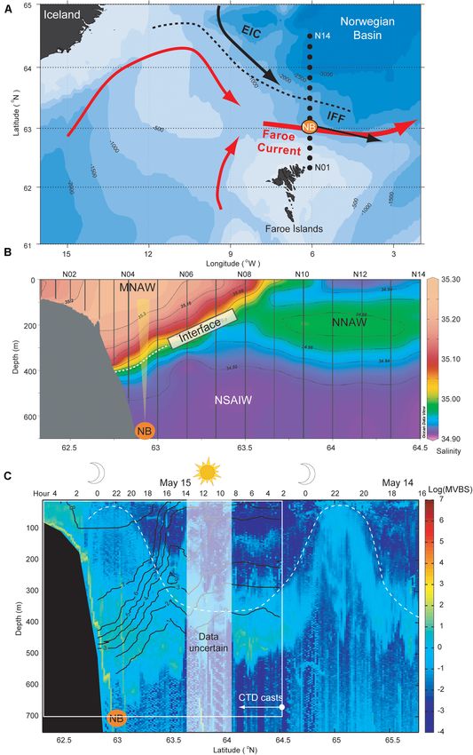
Cisewski et al.                                                                                                          DVM in the Norwegian Sea

(Proud et al., 2017). In addition, the vertical migration of                (Meganyctiphanes norvegica and Thysanoessa spp.), and
zooplankton and nekton plays an important part in the biological            carnivore amphipods (Themisto spp.). In addition, mesopelagic
pump of the World Ocean, where atmospheric CO2 is transferred               fish species such as Maurolicus muelleri, Benthosema
as biogenic carbon to large depths (Longhurst and Harrison,                 glaciale, mesopelagic shrimps and jellyfish occupy the
1988; Jónasdóttir et al., 2015; Turner, 2015). The migrating                mesopelagic realm of these waters (Skjoldal, 2004)—acoustically
zooplankton and nekton feed in the epipelagic zone during                   identifiable as DSLs (Melle et al., 1993; Torgersen et al., 1997;
night and return to the meso- or bathypelagic zone during                   Knutsen and Serigstad, 2001).
day, thereby increasing the carbon flux to the deeper layers                    In 1988, the Faroe Marine Research Institute (FAMRI)
by excretion, fecal pellet production and mortality at depth                started a monitoring program focusing on the state of the
(Bianchi et al., 2013). The necessity of understanding magnitude            pelagic ecosystem north of the Faroe Islands in the southern
and patterns of the vertical migrations has recently become                 Norwegian Sea, along the so-called Section N (Figure 1). In
pressing. This is mainly due to realization that active carbon              this monitoring program, a number of different biological
transport which is mediated by zooplankton and nekton vertical              and physical parameters have been collected. These include
migrations has to be parameterized in global biogeochemical                 predominantly (1) velocity data and backscatter strength
models (Bianchi et al., 2013).                                              recorded with self-contained Acoustic Doppler Current Profilers
    While the evolutionary drivers of DVM and its influencing               (ADCPs), (2) measurements of the hydrography, (3) vessel-
cues are not clearly understood (Lampert, 1989; Cohen and                   mounted echo-sounder data, and (4) accompanying zooplankton
Forward, 2009), predator avoidance is generally considered to               net hauls. ADCPs can complement conventional net sampling
be the most likely underlying mechanism. Nocturnal upward                   due to their advantages of operating autonomously throughout
migration may allow bathy- or mesopelagic species to feed in                the year without being subject to the issue of avoidance, thereby
the epipelagic zone, and thereby reduce the risk of exposure                providing sufficient resolution in depth and time for reliable
to visually orientated predators during the day (Zaret and                  inference of relevant DVM characteristics (Hovekamp, 1989;
Suffern, 1976; Lampert, 1989). DVM is regarded as a behavioral              Zhou et al., 1994; Burd and Thomson, 2012). The drawback,
response toward a combined set of exogenous environmental                   however, is the reduced ability of species identification and the
cues (Forward, 1988), where daylight seems the most important               quantification of their abundances and biomass.
control. Several zooplankton studies conducted in freshwater                    While most previous long-term studies of vertical migration
and marine environments have shown that the migration times                 patterns in the Norwegian Sea have been restricted to the
typically correspond to the times of rapid light intensity changes          Norwegian fjord system (e.g., Staby et al., 2011, 2013; Dypvik
underwater around dusk and dawn (see Roe, 1974; Forward,                    et al., 2012), we here present results of a long-term study
1988; Haney, 1988; Ringelberg, 1995).                                       conducted in the southern Norwegian Sea. Since vertical
    In this study, we focus on the southern Norwegian Sea, which            migration occurs on diel, seasonal and inter-annual time
is dominated by warm and saline Modified North Atlantic Water               scales, long-term ADCP time series enable an analysis of the
(MNAW) entering the area from southwest, and cold and less                  characteristic patterns of vertical migration over the entire
saline East Icelandic Water (EIW) flowing from the northwest                temporal range. Based on two 1 year records of data retrieved
(Figure 1A). After crossing the Iceland-Faroe Ridge, the MNAW               from a self-contained ADCP moored near the core of the Faroe
continues in a narrow boundary current, the Faroe Current,                  Current on section N from June 2013–May 2015 (Figure 1),
which flows eastward north of the Faroe Islands (Hansen et al.,             we present the seasonal variation of the vertical velocity and
2003, 2010; Hátún et al., 2004). The East Icelandic Current                 the mean volume backscattering strength (MVBS) at a 20 min
transports the EIW southeastwards where it meets the warmer                 resolution. These provide accurate qualitative and quantitative
and more saline MNAW in the southwestern Norwegian Sea.                     information on the vertical migration patterns of mesopelagic
A sharp thermo/halocline, hereafter referred to as the interface,           species in a highly productive part of the Northeast Atlantic.
separates these two water masses (Figure 1B), and its vertical              Overall, the aims of this study are (1) the identification of
position changes on weekly to interannual, time scales (Hátún               DSL and DVM patterns and their seasonal variations and
et al., In Prep; Hansen et al., 2019). This interface outcrops at the       (2) the investigation of environmental conditions and cues
surface as the Iceland-Faroe Front (Figure 1A). We follow the               controlling the vertical and temporal distribution of pelagic and
water mass classification proposed by Read and Pollard (1992).              mesopelagic species.
North of the front, the uppermost 700 m are occupied by colder
and less saline Norwegian North Atlantic Water (NNAW) and
Norwegian Sea Arctic Intermediate Water (NSAIW) (Figure 1B).                MATERIALS AND METHODS
    The Norwegian Sea is highly productive and ecologically
very important for large pelagic fish stocks such as Norwegian              Study Area
spring-spawning herring (Clupea harengus), Atlantic mackerel                Standard Section N is comprised of 14 stations, labeled N01-
(Scomber scombrus), and blue whiting (Micromesistius poutassou)             N14, that extend northwards from the Faroe Islands and into
(Prokopchuk and Sentyabov, 2006). These fish stocks prey                    the Norwegian Sea (Figures 1A,B). The stations are located from
on the large biomasses of zooplankton, predominately the                    62.33◦ N to 64.5◦ N at longitude 6.08◦ W, except for station N14
herbivore copepods Calanus finmarchicus and C. hyperboreus                  which is located at longitude 6.00◦ W. Since 1988, there have been
(Wiborg, 1955; Broms et al., 2009), omnivore euphausiids                    up to four hydrographic cruises each year covering this standard

Frontiers in Marine Science | www.frontiersin.org                       2                                   January 2021 | Volume 7 | Article 542386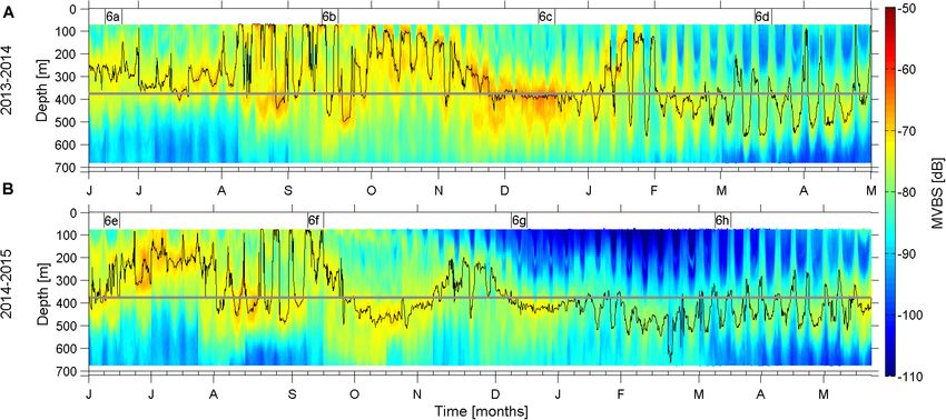
Cisewski et al.                                                                                                                                   DVM in the Norwegian Sea

  FIGURE 1 | (A) Bathymetry and circulation of the study area. Standard hydrographic stations are illustrated as black dots along Section N (06.08◦ W). EIC, East
  Icelandic Current; IFF, Iceland-Faroe Front. The position of ADCP mooring NB is here (and in the panels below) illustrated as an orange dot, and the average
  observed current direction is shown with the black arrow. (B) Average salinity along Section N based on CTD (Conductivity, Temperature, Depth) observation by R/V
  Magnus Heinason in the period June 2013 to May 2015, and the position of the main interface separating warm Atlantic waters from colder underlying waters is
  emphasized. The figure is plotted using Ocean Data View (Schlitzer, Reiner, Ocean Data View, https://odv.awi.de, 2020). (C) acoustic transect along an extended
  Section N during May 14–15, 2018. Data obtained from the ship-mounted echo-sounder on-board R/V Magnus Heinason, are here provided as the mean value
  backscattering strength (MVBS) over 1 m depth intervals and 10 min “distance” (the ship cruises at about 10 knots) intervals. The values are furthermore
  log-transformed, in order to emphasize the diffuse small biota, which are focus of the present study. The position of the 1–8◦ C isotherms, obtained from concurrent
  CTD casts are overlaid with black lines, and the diel vertically migrating layer is emphasized with a white dashed curve. Duration of day and night are illustrated at the
  top of the subfigure, and the white rectangle in (C) outlines the coverage of panel (B). MNAW, Modified North Atlantic Water; NNAW, Norwegian North Atlantic
  Water; NSAIW, Norwegian Sea Arctic Intermediate Water.

Frontiers in Marine Science | www.frontiersin.org                                     3                                            January 2021 | Volume 7 | Article 542386
Cisewski et al.                                                                                                                    DVM in the Norwegian Sea

section. In 1997, the hydrographic data set was complemented                    with a standard calibration sphere (Demer et al., 2015)
by ADCP measurements, which were deployed at depth along                        prior to the surveys.
the section. The core data set of this study consists of ADCP
measurements obtained at standard site NB, which is near the                    Data Analysis
core of the Faroe Current (Figure 1).                                           Computation of Mean Volume Backscattering
                                                                                Strength (MVBS)
CTD Data                                                                        The echo intensities E recorded with the ADCP were given
The hydrographic database consists of conductivity-temperature-                 in an automatic gain control count scale of 0–255. Following
depth (CTD) stations sampled between June 2013 and May 2015                     the version of the sonar equation introduced by Deines (1999)
with a Sea-Bird Electronics SBE 911plus CTD. These stations                     and updated by Mullison (2017), they were converted to the
were used to map the hydrographic field of the Iceland-Faroe                    MVBS (dB):
MNAW inflow toward the Arctic (Hansen et al., 2010). On each
                                                                                  MVBS = C + 10 log (Tx + 273.16)R2 − LDBM − PDBW

cruise, all CTD casts extended down to 1,300 m, except for
shallower stations in the southern part and the northernmost
station on Section N, which extended to 2,000 m. Station spacing                              + 2αR + 10 log 10kc (E−Er )/10 − 1
was equidistantly 10 nautical miles. The CTD has been mounted
with a multi-bottle Sea-Bird SBE32 Carousel water sampler                          with: C = built-in system constant including transducer and
holding 12 5 L bottles. Conductivity data from the CTD probes                   noise features (dB), Tx = temperature of the transducer (◦ C),
were corrected after the cruise with salinity measurements of                   R = range along the beam to scatterers (m), LDBM = 10log10
water samples using a salinometer (Guildline Autosal 8400A)                     (transmit pulse length/meter), PDBW = 10log10 (transmit
referenced to IAPSO standard seawater. The calibration of the                   power/Watt), α = coefficient of sound absorption for seawater
temperature sensor was accurate to < 0.001 K for all surveys.                   (dB/m), kC = beam-specific scaling factor (dB/count). The noise
CTD readings of salinity were calibrated to an accuracy < 0.005.                level (Er ) of all four beams was determined from the minimum
                                                                                values of RSSI (Received Signal Strength Indicator) counts
ADCP Data                                                                       obtained in the remotest depth cell, when the sea surface was
While the ADCP measurements were mainly used to estimate the                    outside the ADCP range. The position of the DSL was estimated
volume transport of MNAW through the standard section (e.g.,                    as the depth at maximum daily (24 h) averaged MVBS within
Hansen et al., 2003, 2010), we here present the first utilization of            the depth range 170–600 m. Similar DSL night- and day- depth
the acoustic backscatter time series measurements derived from a                estimates were obtained when averaging over only the dark
moored 76.8 kHz Workhorse Long-ranger ADCP (Teledyne RD                         hours and the light hours, respectively. As a second approach,
Instruments, United States) to provide valuable insights into the               the weighted mean depth (WMD) of backscatter was used to
dynamics of mesopelagic species. In the study, two consecutive                  determine the mean depth of the DSL. The WMD was calculated
deployments at a standard position between stations N04 and                     for each MVBS profile following the equation:
N05 from the period June 2013–May 2015 have been analyzed
                                                                                                            N                N
(Table 1). In the deployments, the instrument was moored in an                                              X                X
                                                                                                   WMD =          Svi zi /         Svi
upward-looking configuration at ∼700 m depth. The ADCP has
                                                                                                            i=1              i=1
four transducers which are oriented with a slant angle of 20◦ off
the vertical axis. In order to cover the whole water column above               with:     Svi   =     volume         backscattering           coefficient,
the ADCP, it was set to have 70 bins and bin lengths of 10 m. The               zi = corresponding depths.
temporal sampling interval was set to 20 min with 10 equidistant
pings per ensemble; the selected number of pings was based on                   Estimation of the Migration Velocity
the instrument battery consumption.                                             We analyzed the seasonal variation of the migration velocity by
                                                                                calculating average diel cycles of the vertical velocity obtained
Ship-Mounted Echo Sounder Data                                                  by the ADCP for consecutive months (see Figure 7). For
During May 14–15, 2018, a combined acoustic-hydrographic                        improved statistical significance when analyzing vertical velocity,
(CTD) transect was made by FAMRI’s research vessel, R/V                         we averaged the diel cycles between depths of 100 and 500 m.
Magnus Heinason, following Section N and extending further                      Because the uncertainty of single-ping data from the ADCP in
north to 65.8◦ N. The acoustic data were collected from                         the velocity is too large, averaging is applied in order to reach
calibrated scientific echo sounders (Simrad EK60) using an                      acceptable levels. A single-ping uncertainty reading 118 mm s−1
operating frequency of 38 kHz. All transducers are calibrated                   is provided by the manufacturer for the instrument provided in

TABLE 1 | ADCP deployments between station N04 and N05 on Section N (see Figure 1).

Deployment           Latitude         Longitude     Bottom depth (m)        Instrument depth (m)       Observational period                 Duration (days)

1                    62.91◦ N           6.08◦ W            964                        710              June 9, 2013–May 15, 2014                 341
2                    62.92◦ N           6.08◦ W            953                        700              June 6, 2014–May 25, 2015                 354

Frontiers in Marine Science | www.frontiersin.org                           4                                     January 2021 | Volume 7 | Article 542386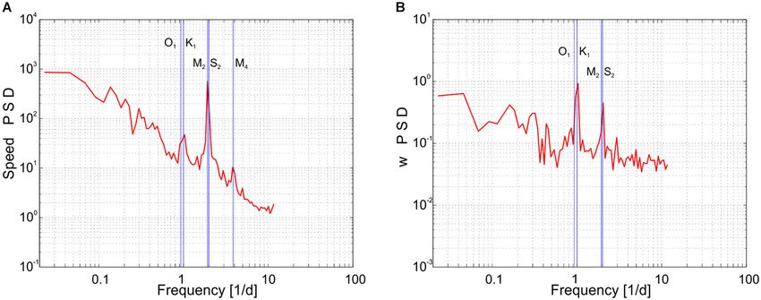
Cisewski et al. DVM in the Norwegian Sea
Range (m)
long-range mode and a bin length of 10 m. Since individual pings
290–600
240–600
70–380
70–380
are independent, measurement uncertainty can be reduced by the
following equation (Teledyne RD Instruments, 2018):
Max
Statistical uncertainty for one ping
+36
+46
+36
+46
+30
Spring equinox
(mm s−1 )
Descent
velocity
p
Number of Pings
Mean
+19
+15
+19
+15
+16
The sampling interval was set to 20 min with 10 pings averaged
per ensemble i.e. 30 pings per hour. For weekly averages, the
Max
−36
−46
−36
−46
−30
number of pings is therefore 7·24·30 = 5,040 and the statistical
(mm s−1 )
velocity
Ascent
uncertainty of the velocity measurements reduces the standard
√
errors of [118/( 5,040 mm s−1 )] = 1.7 mm s−1 . Vertical
Mean
−19
−15
−19
−15
−16
migration velocities are also estimated from the “slope” velocity of
Range (m)
individual MVBS contours, using the method introduced by Luo
70–210
70–210
et al. (2000) and used by Cisewski et al. (2010). The migrating
layer of enhanced MVBS is fit by either a hyperbolic tangent
TABLE 2 | Mean and maximum slope velocities, as well as range of migrating scatterers estimated from the slope velocities of the different scattering layers.
function or a parabolic function. Vertical migration velocities
were then calculated between each successive data point as the
Max
+21
+21
+21
Winter solstice
(mm s−1 )
Descent
velocity
change in depth (m) per time (s). The downward migration phase
of the parabolic fit is defined as the time range that runs from
Mean
+11
+11
+11
the starting point to the vertex of the parabola, and the upward
migration phase as that from the vertex to the endpoint. In the
case of the hyperbolic tangent fit, we define the starting point
Max
−21
−21
−21
(mm s−1 )
velocity
Ascent
and the endpoint as that depth where the change in depth of two
successive data points exceeds 0.5 m. Table 2 gives an overview of
Mean
−11
−12
−11
the estimated velocities.
Range (m)
70–160
70–300
70–160
70–300
Analysis of the Vessel-Mounted Echo Sounder Data
The echo-sounder data were scrutinized using the software
Echoview . Scrutinization involves identifying and aggregating
R
Autumnal equinox
acoustic data, based on knowledge gained from previous repeated
Max
+34
+34
+21
+8
+8
(mm s−1 )
Descent
velocity
visits of the area and from aimed mid-water trawling on the
acoustic targets, segregating the data into regions of identifiable
Mean
+12
+13
+4
+4
+8
fish species. The echo-sounder data were averaged into 1 m ×
10 min (1–2 nautical miles, with the typical cruise speed of the
vessel) bins, providing MVBS.
Max
−34
−34
-21
−8
−8
(mm s−1 )
velocity
Ascent
Interface Depth
Mean
−12
−12
−4
−4
−8
The ADCP mooring is located near the core of the Faroe
Current (Figure 1), and the eastward current component (U-
Range (m)
70–150
70–150
component) gives a valid representation of the mean flow, which
generally is directed slightly south of due east (Figure 1A).
We estimate the vertically undulating lower boundary of the
Faroe Current—the interface—as the depth where the vertical
Max
Summer solstice
+8
+7
+7
(mm s−1 )
Descent
velocity
U-profile is most flat, i.e., locating the maximum of the gradient
dU/dz, where z is depth. Daily averaged U-profiles are used in
Mean
+4
+4
+4
order to avoid the complexity of tides, and only days when the
Faroe Current jet strikes the mooring (criteria: currents at 200
m > 2 × currents at 500 m) have been utilized. Data from both
Max
−8
−7
−7
(mm s−1 )
velocity
deployments have been used for this test, providing 515 daily
Ascent
profiles of the vertically shaped Faroe Current and the same
DSL values in Italics.
Mean
−4
−4
−4
number of interface depths. Direct observations of the interface
depth using a Pressure Inverted Echo Sounder (PIES) (2017–
2013–2014
2014–2015
2019, Hansen et al., 2019) confirms that the U-profile interface
Average
Period
depth estimate closely reflects the vertical variability of the 4◦ C
isotherm (R = 0.64) over the mooring.
Frontiers in Marine Science | www.frontiersin.org 5 January 2021 | Volume 7 | Article 542386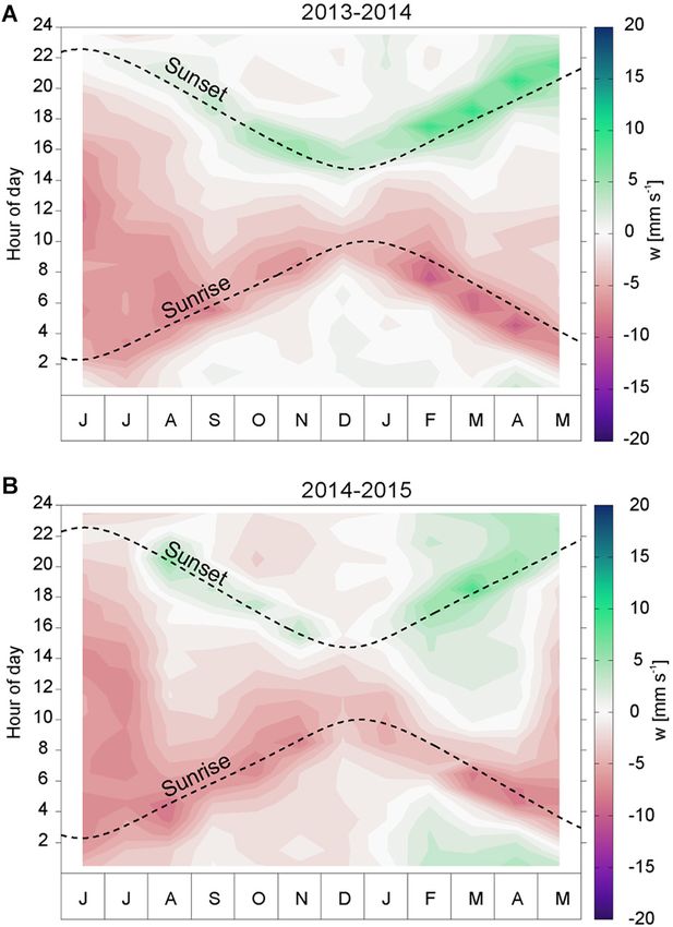
Cisewski et al. DVM in the Norwegian Sea
RESULTS ADCP mooring site (horizontal line at 380 m in Figure 2),
although the DSL was elevated above this depth during summer
Hydrography 2014 (Figure 2B). No statement can be made about the dynamics
Section N extends meridionally from the Faroe Shelf to the in the top few tens of meters, because of the limited reach of the
southern Norwegian Sea. The typical properties of this standard ADCP data. We will hereafter first address the slowly varying
section are illustrated by the averaged salinity from the seven DSL, and then discuss the seasonally varying DVM.
occupations of the section in the observational period June
2013 to May 2015 in Figure 1B. The southern part of this A Close Link Between the DSL and the
transect is dominated by a wedge of warm and salty MNAW Interface
extending horizontally from 62.33 to 63.25◦ N (station N01–N07) The fact that the daytime residence layer—the DSL was located
and vertically from an average of 400 m to the surface. Strong at 400–500 m depths, both within the Faroe Current and far
gradients both in salinity and temperature mark the position north of it during the 2 days of the ship-mounted echo sounder
of the main interface between overlying MNAW and the cold transect (Figure 1C, 14–15 May, 2018) could indicate a broad
and low-saline underlying subarctic water masses. The interface light-regulation of the vertical position of the DSL. On the other
outcropped—average (2013–2015)—at the surface in the vicinity hand, the intensified backscatter at the base of the Faroe Current,
of standard hydrographic station N09, as the Iceland-Faroe Front. whose closely aligned isotherms during these days intersected the
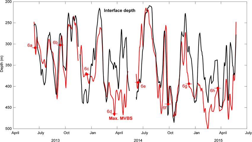
The average depth of the interface at the ADCP mooring site was Faroe slope at 450–500 m depths (Figure 1C), could indicate an
about 380 m (Figure 1B). additional link to the physics of this current. The DSL position at
the ADCP mooring is clearly associated with the interface under
A Ship-Mounted Echo Sounder Transect the Faroe Current (see section “Interface Depth” and Figure 3).
A broad view of the distribution of backscatter-inducing biota This link is very close during the latter half of the year (June–
north of the Faroe slope is provided by the vessel-mounted echo January, R = 0.82), but less direct during the late winter/early
sounder transect along Section N and further north to 65.8◦ N spring months, February to April (R = 0.66). The interface was
(Figure 1C). The research vessel started in the north on May elevated far above its mean depth during July 2014, which can
14, 2018 and the lateral longitude axis (x-axis) is therefore also explain the above mentioned shallow DSL position during this
a time axis increasing southward, with the duration of night and month (Figure 2B).
daytime illustrated above the figure. In addition, CTD casts were The 515 current profiles from the ADCP deployments were
made and isotherms have been overlaid in order to portray the first aligned to the vertically undulating interface reference frame
position of the Faroe Current during those days. A DSL is evident (centered at the steepest dU/dz gradient). Then all the profiles
throughout this transect at 300–500 m depths. The backscatter were averaged, in order to illustrate the mean vertical structure
in this layer is, however, stronger and reaches deeper within the of this flow, relative to the interface depth (Figure 4). This shows
Faroe Current compared to the region farther north. On top of that the eastward flow increases from ∼50 mm s−1 20 m below
this, there is a diffuse scattering layer which exhibits DVM— the interface to ∼130 mm s−1 20 m above the interface. The
located in the near-surface layer during night and congregating in MVBS profiles were similarly aligned to the interface reference
a deep layer during daytime (dashed line in Figure 1C). North of frame and averaged, which reveals that the DSL (MVBS peak) is
the current, the DSL empties when the biota ascends toward the typically located around 10–30 m below the interface depth under
surface at night. Within the Faroe Current, on the other hand, the Faroe Current (Figure 4).
elevated MVBS values were observed both within the DSL and
near the surface during the night.
Diel Vertical Migration
In addition to stochastic motion, short term variability in ocean
Long-Term and Diel Variation in the currents around the Faroe Islands are primarily influenced by
Vertical Distribution of MVBS the semi-diurnal tidal constituents M2 (12.42 h, 1.93 cpd), S2
Mean 24-h cycles of the MVBS vertical distribution (with each (12 h, 2.00 cpd), and N2 (12.66 h, 1.90 cpd) and secondarily
cycle derived from 1 week of data) for 98 consecutive weeks by the diurnal constituents O1 (25.82 h, 0.93 cpd) and K1
(June 2013 to March 2015, Figure 2) reveal a variety of bands (23.93 h, 1.00 cpd) (e.g., Larsen et al., 2008). Distinct elevations
of high backscatter. The mean weighted depth (MWD), overlaid of energy neighboring the semi-diurnal tides M2 and S2 are
the depth-time color image, illustrates the combined variability visible in the power spectra of the horizontal current speed
of two dominant patterns (i) a long term (>a week) variability at the ADCP mooring, followed by a secondary peak at the
of both the intensity and depth of the DSL and (ii) clear diurnal tidal frequencies (O1 and K1 , Figure 5A). In contrast, a
DVM, whose activity varies through the year. The DVM is diel peak dominates the power spectrum of the vertical velocity
most pronounced during the later winter/spring months March- (w), while the semidiurnal constituents represent less energy
April, albeit also invigorated during the fall (late August and (Figure 5B). The enhanced diel energy of w is likely linked to the
September). The DVM activity is relaxed during mid-summer day-night cycle.
(June–July) and mid-winter (November and December). During Complex interplay between the slowly undulating
these seasons, the highest MVBS is observed at the DSL, which DSL/interface and the rapid, although seasonally varying,
generally is located at the mean depth of the interface at the DVM during the years summer 2013–summer 2015 (Figure 2), is
Frontiers in Marine Science | www.frontiersin.org 6 January 2021 | Volume 7 | Article 542386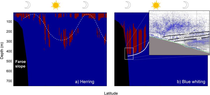
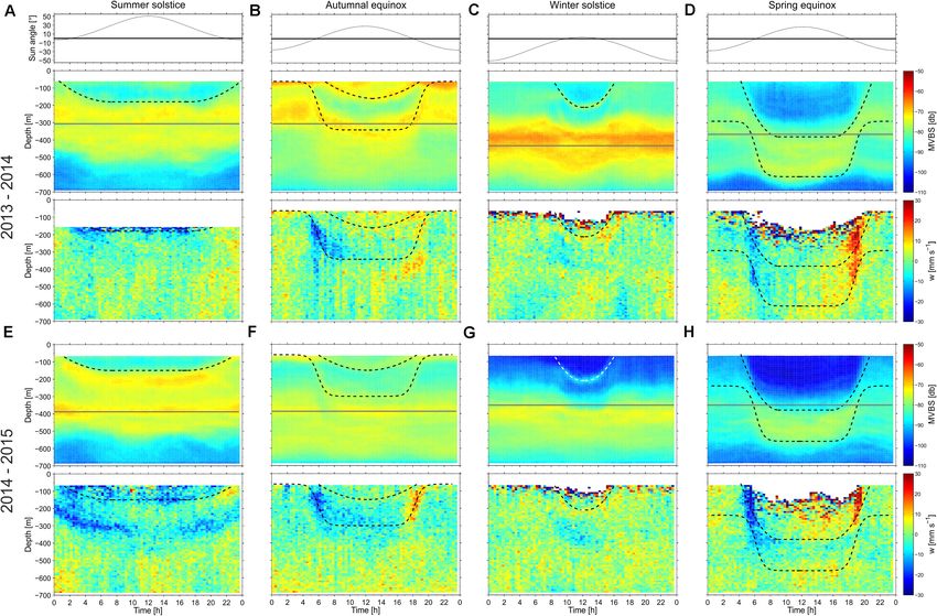
Cisewski et al.                                                                                                                              DVM in the Norwegian Sea

  FIGURE 2 | Annual time series of weekly averaged 24 h cycles of mean volume backscatter strength from June 2013 to May 2014 (A) and from June 2014 to May
  2015 (B), i.e., each weekly slot shows the average 24 h cycle of that week. Overlaid is the weighted mean depths (WMD) (black lines). The Figures 6A–H at the top
  of the panels refer to the weeks, illustrated in the corresponding Figure 6 panels. The average depth of the interface (∼380 m, see Figure 1B) is illustrated with a
  horizontal gray line.

  FIGURE 3 | Temporal variability of the depth of the interface (black) and the strongest mean volume backscattering strength MVBS (red) based on the ADCP
  deployments near the core of the Faroe Current jet. A 5 days low-pass filter has been applied to the daily averaged data. The red strikethrough dots and the
  associated labels refer to the days, illustrated in the corresponding panels in Figure 6.

here discussed for the four distinct seasons: Summer solstice (20–                     to the sun angle calculated using the solar position algorithm by
21 June), autumnal equinox (22–23 September), winter solstice                          Reda and Andreas (2004) (shown in the top panels in Figure 6),
(20–22 December) and spring equinox (20 March). Weekly mean                            and the directly observed vertical velocity, w (lower panels
diel MVBS patterns over these seasons are discussed, in relation                       in Figure 6). The approximate depth of the DVM layers are

Frontiers in Marine Science | www.frontiersin.org                                  7                                           January 2021 | Volume 7 | Article 542386
Cisewski et al.                                                                                                                     DVM in the Norwegian Sea

                                                                                      layers—a slowly migrating layer to 100–150 m depths and a faster
                                                                                      layer reaching 300 m depth during noon (see Table 2). This
                                                                                      deeper DVM seems to have reached, and potentially crossed,
                                                                                      the interface during 2013 (Figure 6B), while it only approached
                                                                                      the interface during 2014 (Figure 6F). During 2014, both the
                                                                                      descending and ascending motion of the deeper DVM layer
                                                                                      was clearly captured by the vertical velocity data (Figure 6F).
                                                                                      Negative values of w also coincided with the descending
                                                                                      scattering layer during 2013 (Figure 6B), while positive w values
                                                                                      were located slightly below the rising layer this year.

                                                                                      Winter Solstice (Sunrise:10:00, Sunset: 14:45, UTC)
                                                                                      A marked and stationary DSL was associated with the interface,
                                                                                      which was located at nearly 400 m depth during both years
                                                                                      (Figures 6C,G), and high MVBS values were observed below
                                                                                      500 m. DVM is evident in the upper 200 m, where waters are
                                                                                      cleared for backscatterers during the few sunlit hours. A slight
  FIGURE 4 | Currents and backscatter at the ADCP mooring near the core of
                                                                                      depression is identifiable in the near-interface DSL during the
  the Faroe Current jet. The averaged (2013–2015) zonal current velocity              lit hours, although the associated motion is too weak for an
  profiles (U-component, black) and the normalized mean volume                        estimation of vertical migration velocities using the curve fitting
  backscattering strength MVBS (red, not to scale), both vertically centered at       method (section “Estimation of the Migration Velocity”). The
  the vertically shifting interface under the Faroe Current (Figure 3).
                                                                                      vertical velocity data (w) do not reveal any discernible patterns
                                                                                      during this season.
emphasized with dashed curves, and identical curves drawn for                         Spring Equinox (Sunrise:6:19, Sunset: 18:45, UTC)
both years, which illustrates the recurrence of the here discussed                    This is the season with strongest DVM, and the interface is only
dynamics. Gray horizontal lines in each subpanel in Figure 6                          vaguely associated with elevated values of MVBS (Figures 6D,H).
represent an approximate position of the interface during the                         Two distinct DVM layers are evident—one migrating from the
8 weeks, highlighted in Figure 3.                                                     near-surface to about 380 m, and a deeper layer that approaches
Summer Solstice (Sunrise: 02:18, Sunset: 22:34, UTC)                                  600 m depth during noon. The shallower layer approaches the
A broad band of strong MVBS is observed in the 300–500 m                              interface, while the deeper migrators approach a deep DSL during
depth interval—with a tendency of congregation at the interface                       noon which, especially in 2014 (Figure 6D), also was occupied
(Figures 6A,E). Low MVBS values are observed below 500 m.                             by biota during the night. During the dark hours, at least a
A DVM layer descends from the near-surface photic zone (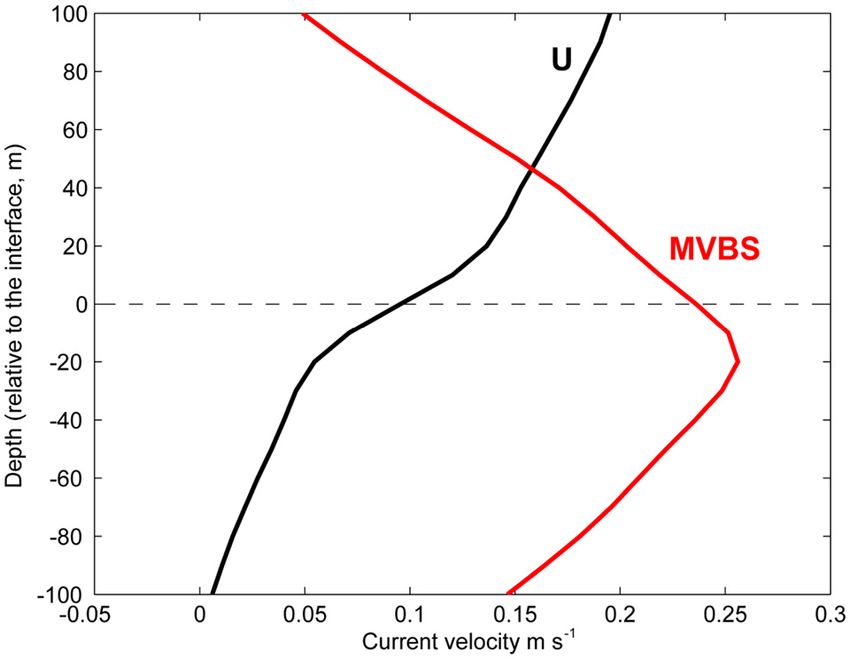
Cisewski et al.                                                                                                                               DVM in the Norwegian Sea

  FIGURE 5 | Power Spectral Densities computed using horizontal current speeds (A) and vertical velocities (B) obtained by the moored ADCP averaged vertically
  between 100 and 200 m. Labels were given to single peaks at tidal constituent frequencies (O1, K1, M2, S2, and M4).

  FIGURE 6 | Mean diel cycle of the sun angle (upper panels), mean volume backscattering strength MVBS (mid-panels) and Doppler vertical velocity w (lower panels)
  estimated for four different weeks near (A,E) summer solstice, (B,F) autumnal equinox, (C,G) winter solstice and (D,H) spring equinox of the years 2013–2015. The
  average interface depth over each individual week (see Figure 3) is illustrated with a horizontal gray line, and the discussed backscatter layers are emphasized with
  dashed curves.

between July and winter solstice, the downward and upward                              band in Figure 7). Similarly, the highest upward velocities
migration peaks shifted by around ± 1 h per month. The                                 are observed after sunset, and the ascent ceases about 1–2 h
scatterers start to descend about 1–2 h before sunrise, and                            after sunset (green band). Negative values of w, related to
highest downward velocities are observed prior to sunrise (red                         downward migration, are evident throughout the year, with

Frontiers in Marine Science | www.frontiersin.org                                  9                                           January 2021 | Volume 7 | Article 542386
Cisewski et al. DVM in the Norwegian Sea
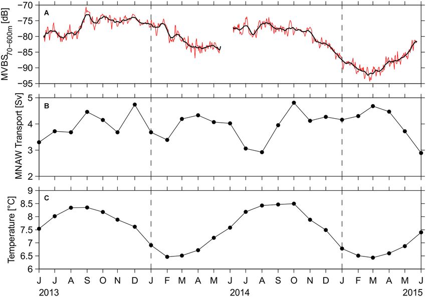
backscatter and temperature values are observed during spring
(6.34◦ C, Figure 8C) and the highest values around August-
September (8.5◦ C). During the sampling period, the MNAW
transport across Section N was relatively persistent, with an
average of 3.8 Sv (Figure 8B), and no clear relation was found
between the MVBS (Figure 8A) and the variability of this
transports (Figure 8B).
DISCUSSION
The presented MVBS data have revealed three dominant
variability patterns: (i) a seasonal cycle of the depth-averaged
backscatter (70–600 m), with a maximum during the late summer
and a minimum during late winter/spring, (ii) a marked DSL
exhibiting relatively slow vertical undulations (>1 month time
scale) within the 250–450 m depth range, and (iii) DVM, which
are active during spring and fall, and more quiescent during mid-
summer and mid-winter. These signals must somehow be related
to lateral transports of MNAW over the main interface, lateral
transports of subarctic water masses under the interface, and/or
vertical migration-motivating cues.
Physical Drivers of the Main Signals
No link is found between the depth-integrated MVBS and the
transport of MNAW, while the MVBS maximum during spring
concurs with minimum in transport-averaged temperature of
the MNAW, and minimum in backscatter during fall concurs
with the highest temperatures. The presented records are,
FIGURE 7 | Seasonal variation of the diel vertical migration velocity averaged however, too short for making any firm conclusions on
between 100 and 500 m depth from June 2013 to May 2014 (A) and from long-term co-variability.
June 2014 to May 2015 (B). Contour intervals are 1 mm s-1. Dashed lines The variable depth of the DSL is linked to vertical undulations
show the times of local sunrise and sunset.
of the interface, with the highest backscatter located immediately
below the interface. This DSL-interface link is likely due to
the accumulation of biomass (backscatters) along the interface,
an indication of higher values during late winter months
more so than a physical reflection from the sea water density
(February to April). During the summer months (June and
gradient across it. It is very close during summer and fall
July) downward velocities are observed in the upper 200 m
and less direct during late winter and spring, when the DVM
of the water column through most of the 24 h cycle. The
activity is strongest (see below). By associating the DSL-
ascent velocities are highest during the late winter and spring
interface link with a recently discovered coupling between the
months (December–May, green) and barely visible during late
interface depth and the circulation strength of the Norwegian
summer and fall.
Sea Gyre (NSG) (Hátún et al., In Prep), we are able to
view this MVBS pattern in a larger oceanographic context.
Depth-Averaged MVBS and A strong (weak) NSG, induced by cyclonic anomaly of the wind
Characteristics of the Faroe Current stress curl of the Norwegian Sea, is associated with a shallow
Daily means of MVBS, averaged between 70 and 600 m water (deep) interface and thus also a shallow (deep) DSL. Also, a
depth, were calculated in order to investigate the seasonality of recently discovered Iceland-Faroe Slope Jet (IFSJ), running at
mesopelagic biomass. The vertically averaged MVBS time series, depth under the Faroe Current, is seen to impact the Faroe
(Figure 8A) reveals a clear seasonal cycle with maximum during Current interface (Semper et al., 2020). Thus an intensified
late summer (August-September), and a minimum around the IFSJ elevates deep (dense) isopycnals in the vicinity of the
late winter/spring months (February–April). MVBS declined by ADCP mooring (Semper et al., 2020), but the influence of this
about 10 dB from November 2013 to February 2014, while the deep flow on the relatively shallow interface has not yet been
larger decline over the subsequent winter amounted to nearer discussed. We are not aware of any previous study which links
15 dB. This seasonal variability of the MVBS co-varies with the acoustic backscatter signals to major oceanographic features.
monthly mean transport-averaged temperature of the eastward It should, for completeness, be mentioned that short-term
flowing MNAW in the Faroe Current (Figure 8C), estimated by fluctuations of the interface depth (Figure 3) are also associated
a new method introduced by Hansen et al. (2020). The lowest with passing weather systems, tides and meso-scale variability
Frontiers in Marine Science | www.frontiersin.org 10 January 2021 | Volume 7 | Article 542386Cisewski et al. DVM in the Norwegian Sea FIGURE 8 | Seasonal variability in mean volume backscattering strength and related environmental parameters: (A) depth-averaged (70–600 m) mean volume backscattering strength (daily averages as red line and 7 days running mean as black line), (B) monthly averaged transports of Modified North Atlantic Water (MNAW) in the Faroe Current, (C) monthly transport-averaged temperature of the MNAW (Hansen et al., 2020). along the Iceland-Faroe Front (Hansen and Meincke, 1979) absolute intensity of light or the rate of change of light were and a thorough investigation of the controlling mechanisms used as an exogenous stimulus for DVM by the migrators will be complex. because of a lack of further information on the light field DVM is a behavioral response to a combination of exogenous within the water. factors (e.g., light, temperature, salinity, and oxygen) and During summer and winter solstices, we only observe endogenous factors (e.g., sex, age, state of feeding, and changes relatively shallow migration, which is unlikely to interfere with in behavior and physiology) (Forward, 1988). Based on MVBS the interface (Figures 6A,E,C,G). However, the deeper migration and w data from the ADCP, we have demonstrated that normal during autumnal equinox does reach depth levels of the interface DVM—closely related to the astronomical daylight cycles—is a (Figures 6B,F), and the involved species could be motivated by persistent behavioral pattern throughout the year. Our results this sharp water mass boundary. During spring equinox, the thus support the hypothesis for light as the most important shallower DVM layer reaches the interface, while the deeper exogenous cue for the timing of DVM within the Faroe Current, DVM layer descends far below the interface (Figures 6D,H), and and likely also for the southern Norwegian Sea as a whole. This is the migrators could therefore contribute to active vertical carbon in agreement with studies from several disparate regions (Roe, transport in this area. Thus, our results might be useful for a 1974; Forward, 1988; Haney, 1988; Ringelberg, 1995), and as regional parameterization of the DVM in biogeochemical models. an example did Staby et al. (2011) show a similar relationship In summary, the seasonal changes in DVM activity and the between the seasonally changing daylight cycle and the timing depths of different migration layers cannot be explained by of the DVM for Müllers pearlside in Masfjorden Norway. There, light intensity alone, and a better understanding likely requires biota also start to migrate downwards shortly before sunrise a consideration of both the physical environment and the and attain again the surface shortly after sunset (Staby et al., species constituting the backscatter layers (section “Reflections 2011). We can, however, not answer the question whether the on Species Involved in Various Patterns”). Frontiers in Marine Science | www.frontiersin.org 11 January 2021 | Volume 7 | Article 542386
Cisewski et al.                                                                                                                                  DVM in the Norwegian Sea

  FIGURE 9 | Scruitinized acoustic backscatter from the ship-mounted echo-sounder. Distribution of (A) herring and (B) blue whiting. Times of day and night are
  cartooned with a sun and a moon, respectively. The dashed undulating curve in (A) illustrates DVM in the herring distribution and the white line in (B) illustrates the
  position of the interface (see Figure 1C). The inset panel in (B) shows acoustic backscatter, in the location where the interface intersects the seafloor (see
  Figure 1C). This is obtained as a screen shot from the software Echoview R , and the position of the three isotherms is estimated from Figure 1C.

Migration Velocities                                                                      C. finmarchicus within the southern Norwegian Sea, continuous
Our results have shown that the migration velocities and daily                            advection of the larger arctic C. hyperboreus into the study region
residence depths vary from season to season (see Table 2).                                with subarctic waters from the Iceland Sea makes this area
The slopes of the scattering layer, which reached about 200 m                             an important feeding area for pelagic fish during their oceanic
depth during noon, revealed vertical migration with average                               feeding phase (ICES, 2020). During late winter to spring, the
speeds of ± 10–20 mm s−1 and maximum speeds of ± 34 mm                                    overwintering copepod generation ascends to the surface layer
s−1 . The layers reaching down to 600 m exhibited similar                                 (upper ∼50 m) (Kristiansen et al., submitted; Gislason, 2018) and
average speeds while maximum speeds reached ± 46 mm s−1 .                                 are therefore out of reach for the ADCP, where they feed on the
This is roughly in accordance Bianchi and Mislan (2016) who,                              initiated spring bloom and reproduce (e.g., Stenevik et al., 2007;
based on a large number of cruises with ship-borne ADCPs in                               Kristiansen et al., submitted). These prey items are too small
the subarctic regions of the North Atlantic, reported vertical                            to give a direct acoustic signal (e.g., Melle et al., 1993), which
migration velocities of 40–50 mm s−1 .                                                    was also supported by a comparison between presented MVBS
   The directly observed vertical migration velocities in Figure 7                        data and depth-stratified zooplankton data along Section N (see
appear lower than the velocities estimated from the slopes                                Supplementary Figure S1).
(Table 2). This could be due both to vertical and temporal                                   However, we suggest that the increased near-surface
averaging of w, (prior to making the figure), and/or the fact                             zooplankton prey biomass could provide a motivation cue for
that w also represents a background of non-migrating scatterers,                          vertical migration of larger biota, which, in turn, could explain
which will introduce a bias into migration rate estimates yielding                        the increased DVM activity during spring (Figures 2, 6). The
systematically smaller velocities (Plueddemann and Pinkel, 1989;                          westward feeding migration of Norwegian spring-spawning
Heywood, 1996; Luo et al., 2000; Cisewski and Strass, 2016).                              herring during April-May is guided by the concentration of
                                                                                          these copepods (Dalpadado et al., 2000; Broms et al., 2012),
                                                                                          and expert scrutiny of the vessel-mounted echo sounder
Reflections on Species Involved in                                                        data presented in Figure 1C (May 14–15, 2018) shows that
Various Patterns                                                                          herring represented a part of the observed backscatter—
Addressing the ecological significance of our study requires                              both in the near-surface (0–50 m) zone and in the layer
knowledge on possible species involved in the MVBS signals.                               performing DVM between the surface and 200–300 m depths
Identifying species is, as mentioned, a limitation in acoustics-                          (Figure 9A). DVM behavior by herring is previously reported
only studies, and the following discussion is therefore of more                           by e.g. Huse et al. (2012). Backscatter observed within the
generalized character.                                                                    uppermost 200 m of the Norwegian Sea is, in addition
   The copepods C. finmarchicus and C. hyperboreus are key                                to herring, likely composed of Müllers pearlside and krill
species in the pelagic system in the southwestern Norwegian                               (euphausiids); and like herring, Müllers pearlside migrate
Sea, coupling primary production and zooplanktivorous fish                                very close to the surface (closer than the minimum detection
(Dalpadado et al., 2000; Hirche et al., 2001). In addition to                             range of the echo sounder) during night, and down into an

Frontiers in Marine Science | www.frontiersin.org                                    12                                           January 2021 | Volume 7 | Article 542386
Cisewski et al. DVM in the Norwegian Sea intermediate layer at 200–300 m depth during the day (Melle also reveal marked DVM, with timing closely associated with et al., 1993; Torgersen et al., 1997; Knutsen and Serigstad, 2001; the day-night light cycle—descent from the photic zone 1–2 h Staby et al., 2011). before sunrise, and reappearance in the near-surface about 1– Blue whiting also enters the study region during May (ICES, 2 h after sunset. Vertical migration velocities and amplitudes 2020), where they typically occupy MNAW (Monstad, 2004) are highest during spring, when the migration consists of two and perform some DVM within 250 m to 400 m depth distinct layers—a shallower layer reaching the interface level levels (Stensholt et al., 2002; Huse et al., 2012). This general (∼400 m) and a deep layer which descends to 600 m. The DVM distribution is also evident in the scrutinized echo sounder activity is also high during fall, with a deeper layer reaching section (Figure 9B), and even more sharply in the raw acoustic 300–400 m depths and a shallower layer descending to ∼150 m. backscatter data at the location where the main pycnocline During mid-summer and mid-winter, a single layer is observed intersects the seafloor (Figure 9B, inset image). In this image, to migrate down to ∼200 m at noon. This novel knowledge on congregations of blue whiting hover over the interface, while the mesopelagic complex in the study region could potentially a more fine-grained backscatter cloud is evident below the guide sampling of the animal species inducing the marked 4◦ C thermocline (Figure 9B). This cloud is reminiscent of a acoustic signals. DSL, which typically is observed between 400 m and 500 m throughout the eastern part of the Nordic Seas, consisting of euphausiids, shrimps, jellyfish and the mesopelagic fish (Melle DATA AVAILABILITY STATEMENT et al., 1993; Salvanes, 2004; Lamhauge et al., 2008). Similar predator-prey layering is observed in other locations in the The raw data supporting the conclusions of this article will be Norwegian Sea and in the Greenland Sea, with planktivorous made available by the authors, without undue reservation. mesopelagic fish occupying the relatively warm Atlantic water and Calanus spp. avoiding the threat of predation by occupying AUTHOR CONTRIBUTIONS the Arctic intermediate water beneath (Dale et al., 1999). These observations are in support of the predator evasion BC and HH coordinated the production of the manuscript. BC, hypothesis, as the smaller animals might be “hiding” in HH, IK, and KL wrote the overall text. BH, SE, and JJ contributed the colder waters from the predation pressure exerted by significantly to the discussion section. All authors contributed to the blue whiting. the article and approved the submitted version. The seasonal MVBS pattern that revealed stronger signals during the summer/autumn and weaker signals during the late winter periods (Figures 2, 8), could be caused by FUNDING the migratory pelagic species herring and blue whiting that congregate and feed along the productive fronts north of Funding for the ADCP measurements was received from the the Faroes from May to December (Utne et al., 2012; European Union 7th Framework Programme (FP7 2007–2013), Trenkel et al., 2014; Strand et al., 2020). Although mackerel under grant agreement no. 308299 (NACLIM). HH and KL also is found in the near-surface layer (
Cisewski et al.                                                                                                                                           DVM in the Norwegian Sea

REFERENCES                                                                                     Hansen, B., Larsen, K. M. H., Hátún, H., and Østerhus, S. (2020). Atlantic
                                                                                                  Water Extent on the Faroe Current Monitoring Section. Havstovan Nr. 20-03
Bianchi, D., and Mislan, K. A. S. (2016). Global patterns of diel vertical migration              Technical Report. Available online at: http://www.hav.fo/PDF/Ritgerdir/2020/
   times and velocities from acoustic data. Limnol. Oceanogr. 61, 353–364. doi:                   TechRep2003.pdf (accessed December 15, 2020).
   10.1002/lno.10219                                                                           Hansen, B., and Meincke, J. (1979). Eddies and meanders in the Iceland-Faroe
Bianchi, D., Stock, C., Galbraith, E. D., and Sarmiento, J. L. (2013). Diel vertical              Ridge area. Deep Sea Res. A Oceanogr. Res. Pap. 26, 1067–1080. doi: 10.1016/
   migration: ecological controls and impacts on the biological pump in a one-                    0198-0149(79)90048-7
   dimensional model. Glob. Biogeochem. Cycles 27, 478–491. doi: 10.1002/gbc.                  Hansen, B., Østerhus, S., Hátún, H., Kristiansen, R., and Larsen, K. M. H. (2003).
   20031                                                                                          The Iceland-Faroe inflow of Atlantic water to the Nordic Seas. Prog. Oceanogr.
Broms, C., Melle, W., and Horne, J. K. (2012). Navigation mechanisms of herring                   59, 443–474. doi: 10.1016/j.pocean.2003.10.003
   during feeding migration: the role of ecological gradients on an oceanic scale.             Hátún, H., Chafik, L., and Larsen, K. M. (in prep). The Norwegian Sea Gyre.
   Mar. Biol. Res. 8, 461–474. doi: 10.1080/17451000.2011.640689                               Hátún, H., Hansen, B., and Haugan, P. (2004). Using an “Inverse Dynamic Method”
Broms, C., Melle, W., and Kaartvedt, S. (2009). Oceanic distribution and life                     to determine temperature and salinity fields from ADCP measurement.
   cycle of Calanus species in the Norwegian Sea and adjacent waters. Deep                        J. Atmos. Ocean. Technol. 21, 527–534.
   Sea Res. II Top. Stud. Oceanogr. 56, 1910–1921. doi: 10.1016/j.dsr2.2008.                   Hays, G. C. (2003). A review of the adaptive significance and ecosystem
   11.005                                                                                         consequences of zooplankton diel vertical migration. Hydrobiologia 503, 163–
Burd, B. J., and Thomson, R. E. (2012). Estimating zooplankton biomass                            170. doi: 10.1023/b:hydr.0000008476.23617.b0
   distribution in the water column near the Endeavour Segment of Juan de Fuca                 Heywood, K. J. (1996). Diel vertical migration of zooplankton in the northeast
   Ridge using acoustic backscatter and concurrently towed nets. Oceanography                     Atlantic. J. Plankton Res. 18, 163–184. doi: 10.1093/plankt/18.2.163
   25, 269–276. doi: 10.5670/oceanog.2012.25                                                   Hirche, H.-J., Brey, T., and Niehoff, B. (2001). A high-frequency time series
Cisewski, B., and Strass, V. H. (2016). Acoustic insights into the zooplankton                    at Ocean Weather Ship Station M (Norwegian Sea): population dynamics
   dynamics of the eastern Weddell Sea. Prog. Oceanogr. 144, 42–92. doi: 10.1016/                 of Calanus finmarchicus. Mar. Ecol. Prog. Ser. 219, 205–219. doi: 10.3354/
   j.pocean.2016.03.005                                                                           meps219205
Cisewski, B., Strass, V. H., Rhein, M., and Krägefsky, S. (2010). Seasonal variation of        Hovekamp, S. (1989). Avoidance of nets by Euphausia pacifica in Dabob Bay.
   diel vertical migration of zooplankton from ADCP backscatter time series data                  J. Plankton Res. 11, 907–924. doi: 10.1093/plankt/11.5.907
   in the Lazarev Sea, Antarctica. Deep Sea Res. I Oceanogr. Res. Pap. 57, 78–94.              Huse, G., Utne, K. R., and Fernö, A. (2012). Vertical distribution of herring and
   doi: 10.1016/j.dsr.2009.10.005                                                                 blue whiting in the Norwegian Sea. Mar. Biol. Res. 8, 488–501. doi: 10.1080/
Cohen, J. H., and Forward, R. B. (2009). Zooplankton diel vertical migration –                    17451000.2011.639779
   A review of proximate control. Oceanogr. Mar. Biol. Annu. Rev. 47, 77–110.                  ICES (2020). Working Group of International Pelagic Surveys (WGIPS). Dublin:
   doi: 10.1201/9781420094220.ch2                                                                 ICES.
Dale, T., and Kaartvedt, S. (2000). Diel patterns in stage-specific vertical migration         Jónasdóttir, S. H., Visser, A. W., Richardson, K., and Heath, M. R. (2015). Seasonal
   of Calanus finmarchicus in habitats with midnight sun. ICES J. Mar. Sci. 57,                   copepod lipid pump promotes carbon sequestration in the deep North Atlantic.
   1800–1818.                                                                                     Proc. Natl. Acad. Sci. U.S.A. 112, 12122–12126. doi: 10.1073/pnas.15121
Dale, T., Bagøien, E., Melle, W., and Kaartvedt, S. (1999). Can predator avoidance                10112
   explain varying overwintering depth of Calanus in different oceanic water                   Klevjer, T. A., Irigoien, X., Røstad, A., Fraile-Nuez, E., Benítez-Barrios, V. M., and
   masses? Mar. Ecol. Prog. Ser. 179, 113–121. doi: 10.3354/meps179113                            Kaartvedt, S. (2016). Large scale patterns in vertical distribution and behavior
Dalpadado, J., Ellertsen, B., Melle, W., and Dommasnes, A. (2000). Food and                       of mesopelagic scattering layers. Sci. Rep. 6:19873. doi: 10.1038/srep19873
   feeding conditions of Norwegian spring-spawning herring (Clupea harengus)                   Knutsen, T., and Serigstad, B. (2001). Potential Implications on the Pelagic Fish and
   through its feeding migrations. ICES J. Mar. Sci. 57, 843–857. doi: 10.1006/                   Zooplankton Community of Artificially Induced Deep-Water Release of Oil and
   jmsc.2000.0573                                                                                 Gas During DeepSpill_2000 – An Innovative Approach. Fisken og Havet 14, 1-
Deines, K. L. (1999). “Backscatter estimation using broadband acoustic Doppler                    37. Available online at: http://www.imr.no/filarkiv/2003/08/biology_report.pdf/
   current profilers,” in Proceedings of the IEEE Sixth Working Conference on                     nb-no (accessed December 15, 2020).
   Current Measurement (Cat. No.99CH36331), San Diego, CA, 249–253. doi:                       Kristiansen, I., Jónasdóttir, S. H., Gaard, E., Eliasen, S. K., and Hátún, H. (accepted).
   10.1109/CCM.1999.755249                                                                        Seasonal variations in population dynamics of Calanus finmarchicus in relation
Demer, D. A., Berger, L., Bernasconi, M., Bethke, E., Boswell, K., Chu, D., et al.                to environmental conditions in the southwestern Norwegian Sea. Deep Sea Res.
   (2015). Calibration of acoustic instruments. ICES Cooperative Research Report               Lamhauge, S., Jacobsen, J. A., Jákupsstovu, S. H. Í., Valdemarsen, J. W., Sigurdsson,
   No. 326. (Copenhagen: International Council for the Exploration of the Sea),                   T., Bardarsson, B., et al. (2008). Fishery and Utilisation of Mesopelagic Fishes and
   133. doi: 10.17895/ices.pub.5494                                                               Krill in the North Atlantic. (Copenhagen: Nordic Minister Council), 1–36.
Dypvik, E., Klevjer, T. A., and Kaartvedt, S. (2012). Inverse vertical migration and           Lampert, W. (1989). The adaptive significance of diel vertical migration of
   feeding in glacier lanternfish (Benthosema glaciale). Mar. Biol. 159, 443–453.                 zooplankton. Funct. Ecol. 3, 21–27. doi: 10.2307/2389671
   doi: 10.1007/s00227-011-1822-4                                                              Larsen, K. M. H., Hansen, B., and Svendsen, H. (2008). Faroe Shelf Water. Cont.
Foote, K. G. (1980). Importance of the swimbladder in acoustic scattering by fish:                Shelf Res. 28, 1754–1768. doi: 10.1016/j.csr.2008.04.006
   a comparison of gadoid and mackerel target strengths. J. Acoust. Soc. Am. 67,               Longhurst, A. R., and Harrison, W. G. (1988). Vertical nitrogen flux from the
   2084–2089. doi: 10.1121/1.384452                                                               oceanic photic zone by diel migrant zooplankton and nekton. Deep Sea Res.
Forward, R. B. (1988). Diel vertical migration: zooplankton photobiology and                      A Oceanogr. Res. Pap. 35, 881–889. doi: 10.1016/0198-0149(88)90065-9
   behaviour. Oceanogr. Mar. Biol. Annu. Rev. 26, 361–393.                                     Luo, J., Ortner, P. B., Forcucci, D., and Cummings, S. R. (2000). Diel vertical
Gislason, A. (2018). Life cycles and seasonal vertical distributions of copepods in               migration of zooplankton and mesopelagic fish in the Arabian Sea. Deep Sea
   the Iceland Sea. Polar Biol. 41, 2575–2589. doi: 10.1007/s00300-018-2392-4                     Res. I Oceanogr. Res. Pap. 47, 1451–1473. doi: 10.1016/s0967-0645(99)00150-2
Haney, J. F. (1988). Diel patterns of zooplankton behaviour. Bull. Mar. Sci. 43,               Melle, W., Kaartvedt, S., Knutsen, T., Dalpadado, P., and Skjoldal, H. R.
   583–603.                                                                                       (1993). Acoustic Visualization of Large Scale Macroplankton and Micronekton
Hansen, B., Hátún, H., Kristiansen, R., Olsen, S. M., and Østerhus, S.                            Distributions Across the Norwegian Shelf and Slope of the Norwegian Sea.
   (2010). Stability and forcing of the Iceland-Faroe inflow of water, heat                       Available online at: http://hdl.handle.net/11250/105194 (accessed December 15,
   and salt to the Arctic. Ocean Sci. 6, 1013–1016. doi: 10.5194/os-6-1013-                       2020).
   2010                                                                                        Monstad, T. (2004). “Blue Whiting,” in The Norwegian Sea Ecosystem, 263-314, ed.
Hansen, B., Larsen, K. M. H., Hátún, H., Jochumsen, K., and Østerhus, S. (2019).                  Skjoldal (Trondheim: Tapir Academic Press), 559.
   Monitoring the hydrographic structure of the Faroe Current. Havstovan Nr. 19-02             Mullison, J. (2017). Backscatter Estimation Using Broadband Acoustic Doppler
   Technical Report. Available online at: http://www.hav.fo/PDF/Ritgerdir/2019/                   Current Profilers - Updated. Application Note. 8–13 (Teledyne RD Instruments
   TechRep1902.pdf (accessed December 15, 2020).                                                  FSA-031). Available online at: http://www.teledynemarine.com/Documents/

Frontiers in Marine Science | www.frontiersin.org                                         14                                               January 2021 | Volume 7 | Article 542386
You can also read