Machine Learning: what is it and what are its components?
←
→
Page content transcription
If your browser does not render page correctly, please read the page content below
Machine Learning: what is it and what are its components?
                 -- some preliminary observations1

                                              Arnold F. Shapiro
          Penn State University, Smeal College of Business, University Park, PA 16802, USA

                                                     Abstract
       This article focuses on conceptualizing machine learning (ML) concepts. The general topics
       covered are supervised learning based on regression and classification, unsupervised
       learning based on clustering and dimensionality reduction, and reinforcement learning. The
       article begins with an overview of ML, including the types of ML and their components.
       Then, for background, basic concepts associated with ML are addressed. From there on the
       discussion turns to ML algorithms, by topic. Although insurance applications of ML are not
       pursued in this version of the article, at the end of each section is a reference to an insurance
       article that applies the ML algorithm discussed in the section. The article ends with a
       commentary.

1
    The support of the Risk Management Research Center at the Penn State University is gratefully acknowledged.

ARCH2021.1 Shapiro_Machine Learning ... 00e6                                                                      1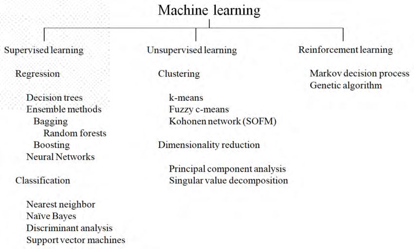
1 Introduction

In the preface to Foundations of modern analysis, Dieudonné (1969) writes that he makes “no
appeal whatsoever to ‘geometrical intuition’... which [he] emphasised by deliberately abstaining
from introducing any diagram in the book.”

Now, if you are a mathematician of the caliber of Dieudonné, you might be of the same mind.
For many, however, forgoing the intuition provided by diagrams and pictures is problematic.
This is a particular concern when dealing with machine learning (ML), where many of the
algorithms are computerized, and it is easy for users to have only a vague notion of the
underlying characteristics of the model they are using.

The current version of this article provides a response to this concern in that it focuses on
conceptualizing machine learning concepts. The final version will expand on notions included in
this draft, and include more details with respect to the underlying mathematics of ML and a
broader overview of insurance applications of ML.

The article begins with an overview of ML, including the types of ML and their components.
Then, for background, basic concepts associated with ML are addressed. From there on the
discussion turns to ML algorithms by type, including supervised learning based on regression,
supervised learning based on classification, unsupervised learning based on clustering,
unsupervised learning based on dimensionality reduction, and reinforcement learning. In each
instance, the emphasis is on conceptualization. Although insurance applications of ML are not
pursued in this version of the article, at the end of each section is a reference to an insurance
article that applies the ML algorithm discussed in the section. The article ends with a
commentary.

2 Machine Learning2
Arthur Samuel (1959), who first conceptualized the notion of machine learning (ML), is often
quoted as defining it as "a field of study that gives computers the ability to learn without being
explicitly programmed." 3 This notion is captured in Figure 1 4, in which traditional programming
and machine learning are juxtaposed, to emphasize the difference between the two:

2
  References for this section include Abellera and Bulusu (2018), Akerkar (2019), Hao (2019), Joshi (2020), KPMG
(2018), Lee (2019), Samuel (1959) and Weng (2015).
3
  This definition should more appropriately be attributed to Samuel because it does not actually appear in the article,
although the sentiment does.
4
    Adapted from Lee (2019) Figures 1.1 and 1.2.

ARCH2021.1 Shapiro_Machine Learning ... 00e6                                                                         2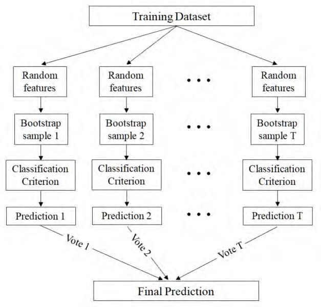
Figure 1: Traditional programming v. ML

As indicated, in traditional programming, the data and the program are the inputs that the
computer uses to produce the output. In contrast, under ML, the data and the output are the
inputs to the computer, which uses them to develop a program to interrelate the two.

2.1 Types of ML
ML is a subset of artificial intelligence (AI). In Figure 2 5 we address the topic of whether the AI
topic under consideration is ML, and, if so, the type of ML.

                               Figure 2: Is it Machine Learning (ML) and, if so, what type?

As indicated, to qualify as ML, it must be seeking a pattern and there must be considerable data
involved. If this is the situation,

      (1) It is supervised learning if it is told what to look for, that is, it is task driven. The
          computer is trained to apply a label to data.

      (2) It is reinforcement learning if trial and error are involved, in which case, the algorithm
          learns to react to the environment. The goal is to discover the best sequence of actions
          that will generate the optimal outcome.

5
    Adapted from Hao (2019).

ARCH2021.1 Shapiro_Machine Learning ... 00e6                                                          3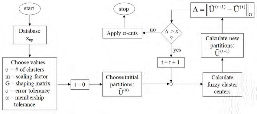
(3) It is unsupervised learning if it is ML but not supervised or reinforcement learning, in
        which case, it is data driven. It discovers patterns or hidden structures in unlabeled data.

3 Algorithms of ML
Figure 3 displays the ML algorithms, by type and subcategory that are discussed in this article,
the details of which are presented in the following pages. The coverage is not exhaustive, in the
sense that not all ML algorithms are addressed, but, hopefully, it is sufficient to provide an
insight into the nature of this area.

                                          Figure 3: ML components

4 Basic concepts associated with ML6
In the following sections, we focus on an explanation of the details of the forgoing ML
algorithms. Before doing that, however, as background, we review two basic concepts associated
with ML: classifier error and bootstrapping.

6
  References for this section include Abellera and Bulusu (2018), Efron (1979), Efron and Tibshirani (1993), Gareth
et al (2013), Knox (2018) and Winston (2010).

ARCH2021.1 Shapiro_Machine Learning ... 00e6                                                                     4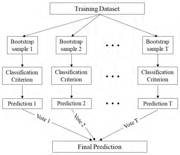
4.1 Classifier error functions
The classification error of a ML algorithm depends on the number of samples incorrectly
classified, including both false positives plus false negatives. In this regard, Figure 4 shows a
representation of a classifier error function. 7
Figure 4: Classifier error function
As indicated, the error rate ranges from 0, which is associated with a strong classifier, to 1,
which is associated with a failed classifier. An important part of the error range is that portion
labeled weak classifier, where the error rate is just under 50%. A classifier that falls into this
category performs better than random guessing, but still performs poorly at classifying objects.
As discussed in §5.2, strong classifiers can be constructed by combining weak classifiers.
4.2 Bootstrapping
Given a dataset and its distribution, the purpose of the bootstrap technique is to generate
additional datasets with similar distributions. It does this by randomly sampling the dataset with
replacement.
The nature of the bootstrap technique can be explained as follows. Let:
x = ( x1 , x2 , , xn ) be n independent data points
x *j = ( xˆ j1 , xˆ j 2 , , xˆ jn ) be the j-th bootstrap sample of size n
Figure 5 provides a representation of the bootstrap process. 8
7
Adapted from Winston (2010).
8
Adapted from Efron & Tibshirani (1993: 13)
ARCH2021.1 Shapiro_Machine Learning ... 00e6 5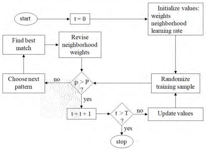
Figure 5: The Bootstrap Process
Given the training dataset, x1 , x2 , , xn , the bootstrap algorithm begins by randomly generating,
with replacement, a large number of independent samples, x*j = ( xˆ j1 , xˆ j 2 , , xˆ jn ) , each of size n. 9
Here, the number of bootstrap samples is B. Moreover, as indicated, corresponding to each
bootstrap sample, j, is a bootstrap replication of the function being investigated, f (x*j ) .
5 Supervised learning based on regression10
This section focuses on the regression algorithms of supervised machine learning, which
model dependencies and relationships between input features and target outputs. The topics
covered are decision trees or CART, ensemble methods, and neural networks.
5.1 Decision Trees or CART 11
"The tree methodology ... is a child of the computer age. Unlike many other statistical
procedures which were moved from pencil and paper to calculators and then to
computers, this use of trees was unthinkable before computers." [Breiman et al (1984:
Preface)]
Decision trees, or Classification and Regression Trees (CART) 12, as they are now commonly
referred to, are decision tree algorithms that are used to resolve classification or regression
predictive modeling problems. These decision trees generally are represented in an upside-down
manner, with their leaves pointed down. Observations pass from the root of the tree through a
9
If, for example, n=5, a random sample, with replacement, might take the form x* = (x2, x4, x1, x1, x2).
10
References for this section include Abellera and Bulusu (2018), Bhatis (2017) and Joshi (2020).
11
References for this subsection include Bisong (2019), Breiman et al (1984), Brownlee (2016), Gareth et al (2013),
Lan (2017), Loh (2014) and Moisen (2008).
12
This term is attributed to Breiman et al (1984).
ARCH2021.1 Shapiro_Machine Learning ... 00e6 6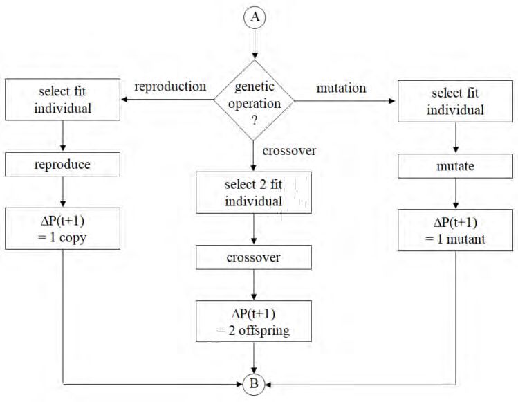
series of nodes, or queries, which, based on the value of an explanatory variables, determine the
subsequent direction of the flow. This process continues until a terminal node or leaf is reached,
at which time a prediction is made. The process is instinctive and easy to understand.

A representation of a feature space and its associated decision tree are depicted in Figure 6(a)
and (b), respectively, 13 where a feature space is the set of possible values associated with features
of a database.

                                 Figure 6: Feature space and associated decision tree

Here, the feature space, X1 and X2, is divided into the distinct and non-overlapping regions, F1,
F2, . . . , F5. Observations that are contained in the latter are assigned the mean of all the
response values of the region. The Xs are considered to be ordered variables if they are
represented by numerical values that have an intrinsic ordering, and categorical variables
otherwise. As indicated, the nodes of the decision tree (the diamond-shaped icons) represent
decision points while the branches, which are binary 14 (yes or no, true or false, etc.) correspond
to possible paths between the nodes.

The allocation of a predicted value to the terminal nodes depends on the type of supervised
learning involved. For regression trees, the terminal node values are allocated based on the mean
for that node. In contrast, for classification trees, the terminal node values are assigned the class
that represents the most cases in that node.

An informative reference for this topic is Loh (2014).

13
     Adapted from Bisong (2019)
14
     The parent node will always split into exactly two child nodes.

ARCH2021.1 Shapiro_Machine Learning ... 00e6                                                          7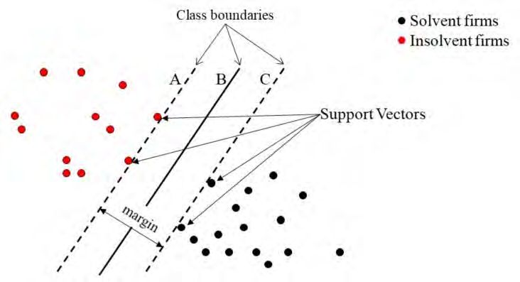
5.2 Ensemble methods
Ensemble, or committee, methods help improve machine learning outcomes by merging machine
learning techniques into a single predictive model. Potential benefits of the method include such
things as decreasing variances and reducing bias. In this subsection, three ensemble methods are
discussed: bagging, random forest and boosting.

5.2.1 Bagging 15

Bagging, is a portmanteau 16 word denoting “bootstrap aggregating.” One of the simpler
ensemble method, its essential characteristic is that samples are taken with replacement, passed
through a classification criterion, and the results thereof are used for prediction. It was first
discussed by Breiman (1996), who envisioned it as a variance reduction technique. The logic
being that the variance of an average is smaller than the variance of the elements of the average.

Figure 7 17 provides a conceptual representation of the bagging technique.

                                            Figure 7: Bagging flowchart

15
  References for this subsection include Breiman (1996), Bühlmann (2012), Bühlmann and Yu (2002), Diana et al
(2019), Knox (2018), Li et al (2018), Winston (2010) and Yuan et al (2018).
16
   Portmanteau is a literary device in which two or more words are joined together to coin a new word, which refers
to a single concept. https://literarydevices.net/portmanteau/
17
     Adapted from Winston (2010) and Yuan et al (2018: 4-5).

ARCH2021.1 Shapiro_Machine Learning ... 00e6                                                                     8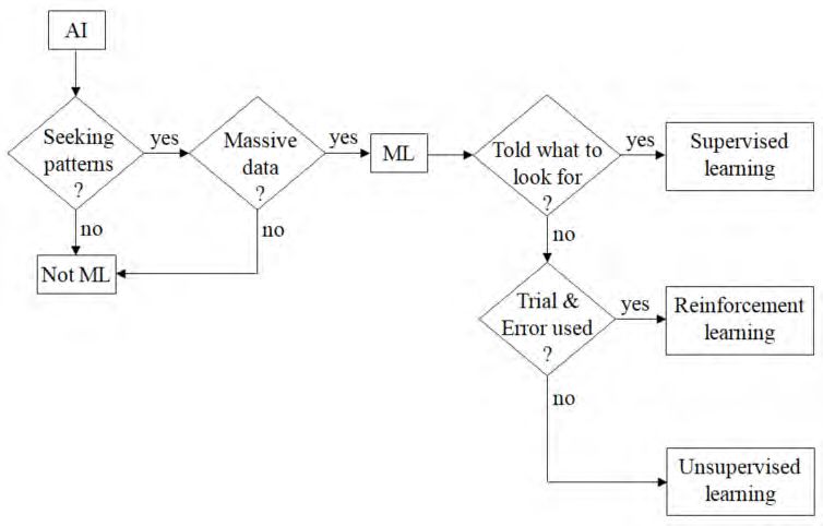
The specific steps can be described as follows:
(1) Use the method of bootstrap to re-sample, and randomly produce T training sets.
(2) Create the corresponding classification criterion for each training set.
(3) For the sample of testing sets, using each classification criterion to test, obtain the T
    predictions.
(4) Based on the method of voting, the prediction with the highest number of votes becomes the
    final prediction.

At its inception, Breiman (1996) gave only heuristic arguments as to why bagging worked.
Subsequently, Bühlmann and Yu (2002) verified that bagging is a smoothing operation that
improves the predictive performance of regression or classification trees, and confirmed
Breiman’s intuition that bagging is a variance reduction technique.

5.2.1.1 Bagging applications in insurance

Li et al (2018) provides an example of a bagging application in insurance.

5.2.2 Random Forests18

       "Random Forests Algorithm [is] identical to bagging in every way, except: each time a
       tree is fit, at each node, censor some of the predictor variables." [Breiman (2011: 12)]

The essential idea behind the random forest concept is that it adds the random selection of
features to the bagging algorithm. The idea was conceived by Ho (1995) 19, who called it
"random decision forest," and described its essence as being "to build multiple trees in randomly
selected subspaces of the feature space." Breiman (2001), who renamed the concept "random
forest" and provided an algorithm for its implementation, is often cited as the originator of the
idea.

Figure 8 20 provides a conceptual representation of the random forest technique.

18
  References for this subsection include Breiman (2011), Derrig and Francis (2005), Diana et al (2019), Ho (1995),
Li et al (2018), Winston (2010) and Yiu (2019).
19
     Apparently, Amit and Geman (1997) also independently conceived the idea.
20
     Adapted from Winston (2010).

ARCH2021.1 Shapiro_Machine Learning ... 00e6                                                                    9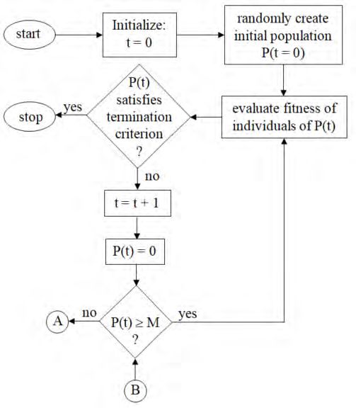
Figure 8: Random forest flowchart
As indicated, the essential modification to the bagging algorithm depicted in Figure 7, and
discussed in the subsequent text, is that only a random subset (without replacement) of the
features are used for each tree.
5.2.2.1 Insurance applications of random forest
Derrig and Francis (2006) provides an example of a random forest application in insurance.
5.2.3 Boosting 21
Boosting is an enhancement of the bagging algorithm that endeavors to improve the learning
process by focusing on areas where the system is underperforming. Under this approach, the first
decision tree is trained on a random sample of data, and the areas that were misclassified are
noted. Then, during the training of the second decision tree, extra weight is given to those
samples where the misclassification occurred. This same sequential procedure continues for the
third and subsequent decision trees, until a stopping criterion is met.
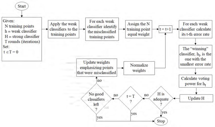
Figure 9 depicts a boosting flowchart.
21
References for this subsection include Bühlmann (2012), Joshi (2020), Kim (2015) and Udacity (2016).
ARCH2021.1 Shapiro_Machine Learning ... 00e6 10Figure 9: Boosting flowchart As indicated, we start with the training points (dataset), the weak classifiers, a strong classifier function, whose initial value is zero, and the potential number of iterations. The weak classifiers, which are given equal weight to start, are applied to the training points, the points that are misclassified are documented, and the error rate of the classifier is determined. The classifiers are assigned a value of 1 or -1 accordingly as the data points that they are applied to are correctly or incorrectly labeled. The weak classifier with the smallest error rate is the winner for that iteration, and its voting power, which is a function of its error rate, is calculated. Then, the strong classifier function is updated by appending the product of the voting power and the sign of the winning weak classifier to its previous value. If the strong classifier is adequate, in the sense that it correctly classifies all the samples, or the iterations have reached their maximum number, or there are no good classifiers left, the algorithm stops. If that is not the case, the weights are updated, with more emphasizing on the points that were misclassified, the sum of the weights is normalized, and the next iteration takes place. 5.2.3.1 Comments Joshi (2020: 62) notes that because of the unavailability of parallel computation, the training of boosted trees is significantly slower than training trees using bagging and random forest. This computational disadvantage notwithstanding, he claims boosting is often preferred over other techniques due to its superior performance in most cases. Bühlmann (2012: 2), on the other hand, remarked that from the perspective of prediction, random forests is about as good as boosting, and often superior to bagging. ARCH2021.1 Shapiro_Machine Learning ... 00e6 11
5.2.3.2 Insurance Applications of Boosting
Guelman (2012) provides an example of a boosting application in insurance.

5.3 Neural Networks 22
       "The traditional approach of capturing first-order behavior has represented a very
       important step toward capturing complex behavior. Now, the use of neural networks that
       can go into the data without any kind of assumption and begin to quantify interactions
       represents the next phase of picking up the higher order terms." [Shapiro (2000: 205)]

Neural networks (NNs) are software programs that emulate the biological structure of the human
brain and its associated neural complex and are used for pattern classification, prediction and
analysis, and control and optimization.

An example of a three layer NN is depicted in Figure 10(a). 23 Here, the first layer, the input
layer, has three neurons 24, the second layer, the hidden processing layer, 25 has three neurons, and
the third layer, the output layer, has one neuron. If the flow of information through the network is
from the input to the output, it is known as a feed forward network. Moreover, if the process
involves supervised learning, in the sense that inadequacies in the output are fed back through
the network so that the algorithm can be improved, the NN is said to involve backpropagation.

                                                Figure 10: A 3-layer NN

22
     References for this subsection include Brockett et. al. (1994) and Shapiro (1998, 1999, 2000 and 2002).
23
     Adapted from Shapiro (2002).
24
     A neuron is a mathematical function that is meant to model the functioning of a biological neuron.
25
  In essence, as observed by Brockett et. al. (1994), p. 408, the "hidden" layers in the model are conceptually similar
to nonorthogonal latent factors in a factor analysis, providing a mutually depend summarization of the pertinent
commonalities in the input data.

ARCH2021.1 Shapiro_Machine Learning ... 00e6                                                                       12
The core of a NN is the neural processing unit, an example of which is shown in Figure 10(b).
As indicated, the inputs to the neuron, nj, are multiplied by their respective weights, wj, and
aggregated. The weight w0 serves the same function as the intercept in a regression formula. 26
The weighted sum is then passed through an activation function, F, to produce the output of the
unit. In the past, the activation function often took the form of a logistic function, F(z)=(1+e-z)-1,
where, as indicated in the figure, z = ∑ j w j x j . Recently, especially where complex hidden
layers are involved, as is the case in deep learning, the Rectified Linear Unit (ReLU), F(z) =
max(0,z), is being used.
The neurons are connected by the weights wijk, where the subscripts i, j, and k refer to the i-th
layer, the j-th node of the i-th layer, and the k-th node of the (i+l)st layer, respectively. Thus, for
example, w021 is the weight connecting node 2 of the input layer (layer 0) to node 1 of the hidden
layer (layer 1). It follows that the aggregation in the neural processing associated with the hidden
neuron n11 results in z = n00 w001 + n01 w011 + n02 w021, which is the input to the activation
function.
A measure of the prediction error in this simple example could be (T-O)2, where T is the targeted
value and O is the output of a given iteration through the network. 27 Now, the weights of the
network serve as its memory and the network "learns" when its weights are updated. To this
end, the prediction error, adjusted by a learning rule, is propagated back through the network so
that the weights can be improved.
5.3.1.1 Insurance Applications of NNs
Brockett et al (1994) provides an early example of a neural network application in insurance.
6 Supervised Learning based on Classification28
This section addresses the problem of supervised learning when the range of the unknown
function is a discrete, unordered set of labels.
Classification is a classic example of supervised learning in insurance. Suppose we have
measured 5 different properties (blood pressure, smoking status, cholesterol ratios, build, and
family history of cancer) 29 of 3 different types of insurance applicants (standard, substandard,
and superstandard). We have measurements for say 1000 different examples of each type of
26
Anders (1996) investigates neural networks as a generalization of nonlinear regression models.
27
The prediction error can be measured in a number of ways. See, for example, Anders (1996, p. 973) and Shepherd
(1997, p 5)
28
References for this section include Abellera and Bulusu (2018) and Knox (2018).
29
See Justman (2007) for a discussion of these factors.
ARCH2021.1 Shapiro_Machine Learning ... 00e6 13applicant. This data would then serve as training data where we have the inputs (the 5 measured
properties) and corresponding outputs (the type of applicant) available for training the model.
Then a suitable ML model can be trained in a supervised manner. Once the model is trained, we
can then classify any applicant (between the three known types) based on the property
measurements. 30
6.1 K-nearest-neighbor (KNN) 31
The essential feature of the k-nearest neighbor algorithm is that it classifies objects on the basis
of their proximity to training examples in the feature space. The underlying logic being that
objects in the immediate vicinity are likely to have similar predictive qualities. As one would
anticipate, and as noted by Akerkar (2019: 24), the method is highly effective when confronted
with noisy or missing training data.
As far as its history, Cover and Hart (1967) are often cited as the early source of the k-NN
algorithm, largely because of their description of how they discovered it. However, the rule was
mentioned by Sebestyen (1962), who labeled it the “proximity algorithm” and by Nilsson (1965)
who labeled it the “minimum distance classifier.” Moreover, as discussed in Pelillo (2014), the
nearest neighbor concept can be traced at least as far back as Alhazen's (1030) Book of Optics.
Figure 11 provides a simple example of a 3-nearest neighbor technique.
Figure 11: 3-nearest neighbor example
In this case, given the 7 data points, comprising two classes, A and B, and a new point x, the 3-
nearest-neighbor (3NN) algorithm classifies x as belonging to the most frequent class of the 3
nearest training data, class B.
Thus, in general, given the training data (x1, y1),…, (xn, yn) and a new point (x, y), the k-nearest-
neighbor (KNN) algorithm classifies (x, y) as belonging to the most frequent class of the k
nearest training data.
30
Adapted from Joshi (2020: 10).
31
References for this subsection include Akerkar (2019), Cover and Hart (1967), Knox (2018), Nilsson (1965),
Pelillo (2014), Sebestyen (1962).
ARCH2021.1 Shapiro_Machine Learning ... 00e6 146.1.1 Insurance applications of k-nearest-neighbor
Dittmer (2006) provides an example of a k-nearest-neighbor application in insurance.
6.2 Naïve Bayes 32
Naïve Bayes, an offshoot of Bayes’ theorem, finds application in high dimensional training data
sets. Its purpose, given the features and classes of a classification problem, is to compute the
conditional probability that an object belongs to a particular class. The algorithm is designated
as naive because it is based on the assumption that the features are independent.
Explicitly, given the classes Ci , i = 1, 2, …, K, and the features xj , j = 1, …, n, the goal is to
calculate the conditional probability that an object with a feature vector (x1, x2, …, xn) is a
member of Ci, that is, P(Ci | x1 , x 2 , , x n ).
Figure 12 33 depicts a simple example involving the Naïve Bayes approach.
Figure 12: Classify 2 new sample using Naïve Bayes
In this case, there are two classes, C1, represented by circles, and C2, represented by squares, and
two new samples, x1 and x2.
The questions at hand are:
What is the probability that the new samples came from each of the classes?
Which class are the samples most likely from?
32
References for this section include Balaji and Srivatsa (2012), Global Software Support, Salma et al (2019) and
Zakrzewska (2008).
33
Adapted from the Global Software Support (2018) example at:
https://www.globalsoftwaresupport.com/naive-bayes-classifier-explained-step-step/
ARCH2021.1 Shapiro_Machine Learning ... 00e6 15Before the new samples, the probability of a circle, P(C1), and a square, P(C2), were 10/15= 2/3,
and 5/15=1/3, respectively.
Now, considering just the neighborhood of the new samples, the area enclosed by the dashed
circle in Figure 12, the probability that the new sample will be a circle or a square will be
P(xi |C1) = 3/10 and P(xi |C2) = 2/5, respectively.
Generalizing, and implementing the Naïve Bayes assumption that
P(x1 , x 2 | Ci ) = P(x1 | Ci ) P(x 2 | Ci )
gives
P(Ci )
=P(Ci | x1 , x2 ) P( x1 | Ci ) P( x2 | Ci ) , 1 ≤ i ≤ K
P( x1 , x2 )
which is the Naïve Bayes version of P(Ci | x1 , x2 ).
6.2.1.1 Insurance applications of Naïve Bayes
Balaji and Srivatsa (2012) provides an example of a Naïve Bayes application in insurance.
6.3 Discriminant Analysis 34
Discriminant analysis, which is based on the means and variances of sets of samples, was
developed to address classification problems where two or more groups or populations are
known a priori and new observations are to be classified into one of the known groups or
populations. In this context, the term "discriminant" refers to a function of a set of variables that
is used as an aid in discriminating between them. There are two types of discriminant analysis:
linear discriminant analysis (LDA) and quadratic discriminant analysis (QDA). These are
discussed in the two subsections that follow.
6.3.1 Linear Discriminant Analysis 35
Linear discriminant analysis (LDA), which can be traced to the early work of Fisher (1936), is
used for classification involving multidimensional normal distributions with homogeneous
variance-covariances. Essentially, given the mean vectors of each class, LDA finds the
projection direction that maximizes separation of means, while taking into account the within-
class variance.
34
References for this portion include Ben-Ari and Mondada (2018) and Timm (2002).
35
References for this subsection include Ben-Ari and Mondada (2018), Knox (2018), Matlab (2018) and Timm
(2002).
ARCH2021.1 Shapiro_Machine Learning ... 00e6 16Figure 13 36 is a representation of a linear discriminant analysis example.
Figure 13: Linear discriminant analysis
As indicated, there are three groups of a priori data. The location of the linear boundaries are
determined by treating the observations of each group as samples from a multidimensional
normal distribution with homogeneous variance-covariance matrices (i.e., Σ1 = Σ2 = Σ3). Given
the fitted distributions, the boundary between the groups are the set of points where the
probabilities are equal, and new observations are classified based on where they occurred relative
to the boundaries.
Discriminants that are linear functions of the variables, as in Figure 13, are called linear
discriminant functions.
6.3.2 Quadratic Discriminant Analysis
Quadratic discriminant analysis is used with heterogeneous variance-covariance matrices, which
allows the variance-covariance matrices to depend on the population.
Figure 14 37 provides a representation of quadratic discriminant analysis.
36
Adapted from Matlab (2018)
37
Adapted from Matlab (2018)
ARCH2021.1 Shapiro_Machine Learning ... 00e6 17Figure 14: Quadratic discriminant analysis
Here, as in the linear discriminant analysis case, the coefficients of the boundary lines are
determined by the mean vectors and covariance matrices of the observed classes. However,
since the covariance matrices are not the same for all classes (i.e., Σ1 ≠ Σ2 ≠ Σ3), the boundaries
are quadratic.
6.3.3 Comment
Bartlett’s test 38 is used to determine if the variance-covariance matrices are homogeneous for all
populations involved and, hence, whether to use Linear or Quadratic Discriminant Analysis.
6.3.4 Insurance applications of discriminant analysis
Riashchenko et al (2017) provides an example of a discriminant analysis application in
insurance.
6.4 Support Vector Machines (SVM) 39
Given a dataset with two target classes that are linearly separable, the objective of a support
vector machine (SVM) is to find the line that best separates the two classes.
A representation of a SVM is shown in Figure 15, in the case where the dichotomy is between
solvent insurance firms and insolvent firms. 40
38
See Keating and Leung (2010).
39
References for this portion include Bisong (2019) and Diepen et al (2017).
40
Adapted from Diepen et al (2017).
ARCH2021.1 Shapiro_Machine Learning ... 00e6 18Figure 15: Support vector machine example In this example, the black and red circles represent solvent firms and insolvent firms, respectively. Any line that keeps the red circles on the left and the black circles on the right is considered a valid boundary line for this classification problem. The two dashed lines are the parallel separation lines with the largest space between them, while the actual classification boundary, which serves as the solution to this SVM problem, since it maximizes the separation between the two classes, is the solid line exactly in the middle of the two dotted lines. The term Support Vector Machine derives from the support vectors that are the basis for the dashed lines in the figure. Here, there are four supporting vectors. 6.4.1 LDA and SVM Although both LDA and SVM are linear discriminant functions, there generally is a clear distinction between them: LDA is concerned with maximizing the distance between the means of the two groups while SVM is concerned with maximizing the margin between the two groups. LDA works best when each of the labeled class data are normally distributed while SVM does not depend on how the data is distributed. On the other hand, SVM and LDA would produce the same result if the data is normally distributed. ARCH2021.1 Shapiro_Machine Learning ... 00e6 19
6.4.2 Insurance applications of SVM

Salcedo-Sanz et al (2003) provides an example of a SVM application in insurance.

7 Unsupervised learning based on clustering
The purpose of unsupervised learning based on clustering is to partition a set of observations into
separate groups or clusters in such a way that all observations within a group are similar, while
observations in different groups are dissimilar. Given this clustering, a new observation can be
compared to the clusters and assigned to the one to which they are most closely aligned.

In the rest of this section we discuss three types of clustering: k-means algorithm, fuzzy c-means
algorithm and self-organizing feature map.

7.1        k-means 41
Given a dataset, the purpose of the k-means clustering algorithm is to arrange the data in k
clusters such that the total within-cluster variation is minimized.

Figure 16 42 shows a simple example of 3-means clustering.

                                             Figure 16 3-means clustering

Starting with the training data in Figure 16(a) and the goal of 3 clusters, 3 points are randomly
chosen, the tentative centroids or centers of mass, one for each cluster. Then, as shown in Figure

41
     References for this portion include Dinov (2018), Jeffares (2019) and medium.com.
42
     Adapted from Jeffares (2019)

ARCH2021.1 Shapiro_Machine Learning ... 00e6                                                    20
16(b), each data point is assigned to the cluster that it is closest to. Next, a new centroid is
located for each cluster based on the current cluster members. Given the new centroids, the
foregoing steps are repeated until convergence occurs, in the sense that the centroids do not
change from one iteration to the next.
7.1.1 Insurance applications of k-means
Hainaut (2019) provides an example of a k-means application in insurance.
7.2 Fuzzy c-means 43
The essence of the c-means algorithm is that it produces reasonable centers for clusters of data,
in the sense that the centers capture the essential feature of the cluster, and then groups data
vectors around cluster centers that are reasonably close to them.
Figure 17 44 shows a flowchart of the c-means clustering algorithm.
Figure 17: c-means clustering algorithm
As indicated, the database consists of the n×p matrix, Xnp, where n indicates the number of
patterns and p denotes the number of features. The algorithm seeks to segregate these n patterns
into c, 2 ≤ c ≤ n - 1, clusters, where the within clusters variances are minimized and the between
clusters variances are maximized. To this end, the algorithm is initialized by resetting the
counter, t, to zero, and choosing: c, the number of clusters; m, the exponential weight, which acts
to reduce the influence of noise in the data because it limits the influence of small values of
membership functions; G, a symmetric, positive-definite (all its principal minors have strictly
positive determinants), p × p shaping matrix, which represents the relative importance of the
elements of the data set and the correlation between them, examples of which are the identity and
43
References for this subsection include Bezdek (1981) and Shapiro (2004)
44
This figure and related discussion follows Shapiro (2004).
ARCH2021.1 Shapiro_Machine Learning ... 00e6 21covariance matrixes; ε, the tolerance, which controls the stopping rule; and α, the membership
tolerance, which defines the relevant portion of the membership functions.
Given the database and the initialized values, the counter, t, is set to zero. The next step is to
choose the initial partition (membership matrix), U (0) , which may be based on a best guess or
experience. Next, the fuzzy cluster centers are computed, which, in effect, are elements that
capture the essential feature of the cluster. Using these fuzzy cluster centers, a new (up-dated)
(t +1) , is calculated. The partitions are compared using the matrix norm U
partition, U (t +1) − U
(t )
G
and if the difference exceeds ε, the counter, t, is increased and the process continues. If the
difference does not exceed ε, the process stops. As part of this final step, α-cuts are applied to
clarify the results and make interpretation easier, that is, all membership function values less than
α are set to zero and the function is renormalized.
7.2.1 Insurance applications of c-means algorithm
Subudhi and Panigrahi (2020) provides an example of a c-means algorithm application in
insurance.
7.3 Kohonen network (SOFM) 45
This section discusses a common unsupervised NN, the Kohonen network (Kohonen,1988),
which otherwise is referred to as a self-organizing feature map (SOFM). The purpose of the
network is to emulate our understanding of how the brain uses spatial mappings to model
complex data structures. Specifically, the learning algorithm develops a mapping from the input
patterns to the output units that embodies the features of the input patterns.
In contrast to the supervised network, where the neurons are arranged in layers, in the Kohonen
network they are arranged in a planar configuration and the inputs are connected to each unit in
the network. This configuration is depicted in Figure 18. 46
45
References for this subsection include Kohonen (1988) and Shapiro (2000b).
46
This figure and related discussion follows Shapiro (2000b).
ARCH2021.1 Shapiro_Machine Learning ... 00e6 22Figure 18: 2-D Kohonen network
As indicated, the Kohonen SOFM is a two-layered network consisting of a set of input units in
the input layer and a set of output units arranged in a grid called a Kohonen layer. The input and
output layers are totally interconnected and there is a weight associated with each link, which is a
measure of the intensity of the link.
The sketch of the operation of a Kohonen network is shown in Figure 19.
Figure 19: Operation of a Kohonen network
ARCH2021.1 Shapiro_Machine Learning ... 00e6 23The first step in the process is to initialize the parameters and organize the data. This entails
setting the iteration index, t, to 0, the interconnecting weights to small positive random values,
and the learning rate to a value smaller than but close to 1. Each unit has a neighborhood of units
associated with it and empirical evidence suggests that the best approach is to have the
neighborhoods fairly broad initially and then to have them decrease over time. Similarly, the
learning rate is a decreasing function of time.
Each iteration begins by randomizing the training sample, which is composed of P patterns, each
of which is represented by a numerical vector. For example, the patterns may be composed of
solvent and insolvent insurance companies and the input variables may be financial ratios. Until
the number of patterns used (p) exceeds the number available (p > P), the patterns are presented
to the units on the grid, each of which is assigned the Euclidean distance between its connecting
weight to the input unit and the value of the input.
The unit which is the best match to the pattern, the winning unit, is used to adjust the weights of
the units in its neighborhood. The process continues until the number of iterations exceeds some
predetermined value (T).
In the foregoing training process, the winning units in the Kohonen layer develop clusters of
neighbors which represent the class types found in the training patterns. As a result, patterns
associated with each other in the input space will be mapped on to output units which also are
associated with each other. Since the class of each cluster is know, the network can be used to
classify the inputs.
7.3.1 Insurance applications of SOFM
Brockett et al (1998) provides an example of a SOFM application in insurance.
8 Unsupervised learning based on Dimensionality
Reduction47
The purpose of dimensionality reduction is to reduce the dimensions of a dataset while
maintaining most of its relevant information. A separate preprocessing step, it reduces the
demand on storage space, improves computational efficiency, and, by reducing exposure to the
curse of dimensionality48, it can improve the predictive performance.
In the rest of this section we discuss two types of dimensionality reduction: principal component
analysis and singular vector decomposition.
47
References for this subsection include Alpaydin (2014), Hoang (2016) and Lorraine (2019).
48
The curse of dimensionality refers to various phenomena that arise when analyzing and organizing data in high-
dimensional spaces that do not occur in low-dimensional settings such as the three-dimensional physical space of
everyday experience. Wikipedia
ARCH2021.1 Shapiro_Machine Learning ... 00e6 248.1 Principal component analysis (PCA) 49
Principal Component Analysis (PCA) is a feature (dimension) extraction method that seeks to
reduce a set of correlated features of a data set to a smaller set of uncorrelated hypothetical
features called principal components (PCs). It does this by focusing on directions of maximum
variance of the data. The rational for a PCA is that if fewer features can be used to represent a
dataset, without significant loss of information, analysis is facilitated.
Figure 20 50 provides a simple example of a PCA application, where x1 and x2 represent the
features.
Figure 20: PC example
It is clear from Figure 20(a) that the x1 and x2 features are highly correlated, which implies
redundancy. This suggests that the two dimensions of data can be reduced to one, with a limited
amount of information loss.
49
References for this subsection include Alpaydin (2014), Ham and Kostanic (2001), Lorraine (2019) and Timm
(2002).
50
Adapted from Abdullatif (2018).
ARCH2021.1 Shapiro_Machine Learning ... 00e6 25To accommodate this, the axes is realigned so that the first principal axis, z1, is in the direction
that produces of the largest possible variance for the dataset and the second principal axis, z2, is
orthogonal to the first. As shown in Figure 20(b), for this example, this results from a 45 degrees
rotation of the axes. Thus, z1 = x1 - x2 (i.e., x1 = x2) and z2 = x1 + x2 (i.e., x1 = - x2).
Now, since the variance of the data along the z1 axis is much larger than the variance of the data
along the z2 axis, PCA suggests that only the principal axis, z1, be maintained. To accommodate
this, the data points are projected onto the z1 axis, as shown by the dashed lines in Figure 20(c).
This results in a 1D dataset in place of the original 2D dataset.
8.1.1 Insurance applications of PCA
Chen et al (2008) provides an example of a PCA application in insurance.
8.2 Singular value decomposition (SVD) 51
Singular value decomposition (SVD) can be thought of as the decomposition of vectors onto
orthogonal axes.
Every matrix A can be factored as A = UΣVT, which is known as the singular value
decomposition of A. In this formulation, Σ is a diagonal matrix, whose entries, the number of
which are equal to the rank 52 of A, are nonnegative numbers called singular values. Similarly,
the columns of U and V, the number of which are also equal to the rank of A, are called left and
right singular vectors, respectively.
Figure 21 53 depicts a representation of SVD in the 2-D case,
51
References for this subsection include Abdullatif (2019) and Math3ma (2020).
52
The rank of a matrix is the maximum number of linearly independent column or row vectors in the matrix.
53
This figure and related discussion is adapted from Abdullatif (2019).
ARCH2021.1 Shapiro_Machine Learning ... 00e6 26Figure 21: a representation of SVD in the 2-D case
where:
a, b ≡ vectors
Sai, Sbi, i = 1, 2 ≡ line segments
vi, i = 1, 2 ≡ unit vectors
In what follows we validate that Figure 21 is a representation of SVD.
From the figure, the length of the projection of sa1 is the dot product of the transpose of a, aT, and
the unit vector v1, that is,
v1x
=a T v1 (a=
x ay) s a1 .
v1y
Thus, more generally, if
ax ay v1x v 2x s a1 s a 2
A= , V = , and S =
bx by v1y v 2y s b1 s b2
then
A⋅V = S or A = S V-1 = S VT . 54
Normalizing the columns of S by dividing them by their magnitudes,
=
σi (s ai ) 2 + (s bi ) 2 , i = 1, 2,
54
If a square matrix is orthogonal, its transpose is equal to its inverse. [Ayres (1962: 103)]
ARCH2021.1 Shapiro_Machine Learning ... 00e6 27gives
sσa1 sσa 2 σ 0 u a1 u a 2 σ1 0
=S = 1 2
1 = U Σ.
sσb1 sσb 2 0 σ 2 u b1 u b2 0 σ 2
1 2
That is, normalizing the columns of S results in the conventional SVD formula
A = U Σ VT.
8.2.1 Insurance applications of SVD
Kossi et al (2006) provides an example of a SVD application in insurance.
9 Reinforcement learning55
Sutton and Barto (2018), in the introduction to their popular book, observed that "Reinforcement
learning ... is a computational approach to learning whereby an agent tries to maximize the total
amount of reward it receives while interacting with a complex, uncertain environment." One
vivid example of this was AlphaGo, the first computer program to defeat a world-class champion
at the game of Go. 56
Operationally, reinforcement learning may be thought of as involving a two-tier process:
exploration and exploitation. At the beginning of the learning process, prior to any knowledge
having been acquired, the system is in its exploration mode, and actions taken by it are random
in nature. In this mode, the results of trying potential actions are documented as to whether they
produce positive, negative, or neutral rewards. Once sufficient feedback is acquired, the system
enters its exploitation mode, where it uses its learned knowledge to produce deterministic, rather
than random, actions.
In this section, two reinforcement learning algorithms are presented that exemplify these
characteristics: Markov decision processes and genetic algorithms.
55
References for this section include Broekens (2007), Joshi (2020), Mnih et al (2016), and Sutton and Barto
(2018).
56
Silver et al (2017) gives an interesting overview of the recent status of reinforcement learning as applied to board
games.
ARCH2021.1 Shapiro_Machine Learning ... 00e6 289.1 Markov decision process 57
A Markov decision process (MDP) is a discrete-time stochastic control process that models
decision making in situations where outcomes are partly random and partly under the control of a
decision maker. It involves a standard reinforcement learning setting, where an agent interacts
with the environment over a number of discrete-time steps. During this progression, the agent
encounters various states and chooses various actions, subject to given policy. As with Markov
chains, the only information available for this decision making is associated with the current
state of the agent. At each new state, the agent receives a reward. The process continues until the
agent reaches a terminal state.
Key parameters of the model, for t = 0,1,2, ..., T, are
S = {st} ≡ a finite set of all the possible decision states,
A = {at} ≡ a finite set of all the valid actions,
P = {pt} ≡ a matrix of state transition probabilities,
R = {rt} ≡ set of all the possible rewards,
Π = {π(at | st)} ≡ set of policy functions that specify the action, at , given st
= {πt}, for short
Figure 22 shows a representation of the role of these parameters in a MDP flowchart over the
time interval t-1 to t+2.
Figure 22: MDP flowchart
57
References for this subsection include Chhabra (2018), Clayton (2011), Marbach (1998), Mnih et al (2016) and
Sloan (2014).
ARCH2021.1 Shapiro_Machine Learning ... 00e6 29Focusing on time t, the system is in state st , the agent takes the action at in response to the policy
function πt, the environment transitions to a new state st+1 with a probability pt, and the agent
acquires reward rt .
9.1.1 Insurance applications of MDP
Dellaert et al (1993) provides an example of a MDP application in insurance.
9.2 Genetic algorithms 58
GAs are automated heuristics that perform optimization by emulating biological evolution. They
are particularly well suited for solving problems that involve loose constraints, such as
discontinuity, noise, high dimensionality, and multimodal objective functions.
GAs can be thought of as an automated, intelligent approach to trial and error, based on
principles of natural selection. In this sense, they are modern successors to Monte Carlo search
methods. The flow chart in Figure 23 59 gives a representation of the process.
Figure 23: Flowchart of a GA
58
References for this subsection include Shapiro (2000a).
59
Figure 23 and Figure 24 were adapted from Shapiro (2000a), Figures 8 and 9.
ARCH2021.1 Shapiro_Machine Learning ... 00e6 30As indicated, GAs are iterative procedures, where each iteration (t) represents a generation. The
process starts with an initial population of solutions, P(0), which are randomly generated. From
this initial population, the best solutions are “bred” with each other and the worse are discarded.
The process ends when the termination criterion is satisfied.
There are three ways to develop a new generation of solutions: reproduction, crossover and
mutation. Reproduction adds a copy of a fit individual to the next generation. Crossover emulates
the process of creating children, and involves the creation of new individuals (children) from the
two fit parents by a recombination of their genes (parameters). Under mutation, there is a small
probability that some of the gene values in the population will be replaced with randomly
generated values. This has the potential effect of introducing good gene values that may not have
occurred in the initial population or which were eliminated during the iterations. The process is
repeated until the new generation has the same number of individuals (M) as the current one.
A flowchart of the process for generating new populations of solutions is depicted in Figure 24.
Figure 24: Reproduction, crossover, and mutation
9.2.1 Insurance applications involving GAs
Yan et al (2020) provides an example of a GA application in insurance.
ARCH2021.1 Shapiro_Machine Learning ... 00e6 3110 Commentary
In this article, we explored the characteristics of some ML algorithms of each type of ML:
supervised learning based on regression and classification, unsupervised learning based on
clustering and dimensionality reduction, and reinforcement learning. In each instance, the focus
was on conceptualization.
As mentioned previously, this version of this article should be viewed as preliminary, in the
sense that subsequent versions will extend the discussion to include:
(1) more details with respect to the underlying mathematics of ML, to complement the
current text,
(2) a broader discussion of the types of ML algorithms, and
(3) an overview of insurance applications related to ML algorithms.
This being a preliminary version notwithstanding, it is hoped that this article stimulates
discussion and provides direction and insight for further research in this area. To the extent it
does so, it will have served its purpose.
References
Abdullatif, H. (2019) "You Don’t Know SVD." https://towardsdatascience.com/svd-8c2f72e264f
Abellera, R., Bulusu, L. (2018) Oracle Business Intelligence with Machine Learning, Springer
Science
Akerkar, R. (2019) Artificial Intelligence for Business, Springer.
Bajaj, C. (2018) "Fisher’s (1936) Linear Discriminant Analysis," Lecture Notes: Geometry of
Spectral Methods for Learning: Linear and Kernel Discriminant Analysis, University of
Texas at Austin.
Bartlett, M. S. (1937) "Properties of sufficiency and statistical tests," Proceedings of the Royal
Statistical Society, Series A 160, 268-282
Bhatis, R (2017) "Top 6 regression algorithms used in data mining and their applications in
industry." https://analyticsindiamag.com/top-6-regression-algorithms-used-data-mining-
applications-industry/
Bisong, E. (2019) Building Machine Learning and Deep Learning Models on Google Cloud
Platform, Springer Science.
Breiman, L. (1996) "Bagging predictors," Machine Learning, 24, 123-140.
ARCH2021.1 Shapiro_Machine Learning ... 00e6 32Breiman, L. (2011) CART, Bagging Trees, Random Forest.
http://civil.colorado.edu/~balajir/CVEN6833/lectures/cluster_lecture-2.pdf
Breiman, L., Friedman, J., Olshen. R., Stone, C. (1984) Classification and Regression Trees,
Chapman and Hall, Wadsworth, New York.
https://www.taylorfrancis.com/books/9781315139470
Brockett, P. L., Cooper, W. W., Golden, L. L., Pitaktong, U. (1994) "A Neural Network Method
for Obtaining an Early Warning of Insurer Insolvency," The Journal of Risk and Insurance,
402-424.
Brockett, P. L., Xiaohua, X., Derrig, R. A. (1998) "Using Kohonen's self-organizing feature map
to uncover automobile bodily injury claims fraud," Journal of Risk and Insurance 65(2), 245-
274.
Bühlmann, P. (2012) "Bagging, Boosting and Ensemble Methods," ETH Zürich.
Bühlmann, P., Yu, B. (2002) "Analyzing bagging," Annals of Statistics 30, 927-961.
Buja, A., Stuetzle, W. (2006) "Observations on bagging," Statistica Sinica 16, 323-351.
Chen, J.-S., Chang, C.-L., Hou, J.-L., Lin, Y.-T. (2008) "Dynamic proportion portfolio insurance
using genetic programming with principal component analysis," Expert Systems with
Applications 35, 273-278.
Chhabra, J. P. S. (2018) Design as a Markov decision process, A Dissertation in Civil and
Environmental Engineering, The Pennsylvania State University.
Dellaert N. P., Frenk, J. B. G., Rijsoort, L. P. (1993) "Optimal claim behaviour for vehicle
damage insurances," Insurance: Mathematics and Economics 12, 225-244.
Derrig, R., Francis, L. (2006) "Distinguishing the Forest from the TREES: A Comparison of
Tree Based Data Mining Methods," Casualty Actuarial Society Forum, Winter, 1-49.
Diana, A., Griffin, J. E., Oberoi, J., Yao, J. (2019) Machine-Learning Methods for Insurance
Applications - A Survey, Society of Actuaries.
Dieudonné, Jean Alexandre. 1969. Foundations of modern analysis, Academic Press
Dittmer, J. M. (2006) "Nearest-neighbour methods for reserving with respect to individual
losses," Blätter 27(4), 647-664.
Fisher, R. A. (1936) "The use of multiple measurements in taxonomic problems," Annals of
Eugenics, 179-188.
ARCH2021.1 Shapiro_Machine Learning ... 00e6 33Francis, L. (2014) "Unsupervised Learning," in E. W. Frees, R. A. Derrig, and G. Meyers (2014)
Predictive modeling applications in actuarial science I, Cambridge University Press, 285-
311.
Gareth, J., Witten, D., Hastie, T., Tibshirani, R. (2013) An introduction to statistical learning,
Springer Science + Business Media, New York.
HackerEarth (2017-04-19) "Introduction to Naïve Bayes Theorem."
https://www.youtube.com/watch?v=sjUDlJfdnKM
Hainaut, D. (2019) "A self‑organizing predictive map for non‑life insurance," European
Actuarial Journal 9, 173-207.
Bor Harej, B., Gächter, R., Jamal, S. (2017) "Individual Claim Development with Machine
Learning," ASTIN, 1-36.
Ho, T. K. (1995) "Random Decision Forests," Proceedings of the 3rd International Conference
on Document Analysis and Recognition, Montreal, QC, 14–16 August, 278-282.
Keating, J. P., Leung, M. T. (2010) "Bartlett's Test," Encyclopedia of Research Design, Sage
Publications, 61-64.
Koissi, M.-C., Shapiro, A. F., Högnäs, G. (2006) "Evaluating and extending the Lee-Carter
model for mortality forecasting: Bootstrap confidence interval," Insurance: Mathematics and
Economics 38(1), 659-675.
Kohonen, T. (1988) Self-Organization and Associative Memory, 2nd Edition. Springer, New
York.
Kurama, V. (2020) A Guide To Understanding AdaBoost.
https://blog.paperspace.com/adaboost-optimizer/
Lan, H. (2017) Decision Trees and Random Forests for Classification and Regression pt.1
https://towardsdatascience.com/decision-trees-and-random-forests-for-classification-and-
regression-pt-1-dbb65a458df
Lee, W.-M. (2019) Python Machine Learning, John Wiley & Sons, Inc.
Lia, Y., Yana, C., Liub, W., Lica, M. (2018) "A principle component analysis-based random
forest with the potential nearest neighbor method for automobile insurance fraud
identification," Applied Soft Computing 70, 1000-1009.
Loh, W.-Y. (2014) "Fifty years of Classification and Regression Trees," International Statistical
Review 82(3), 329-348.
Math3ma (2020) Understanding entanglement with SVD,
ARCH2021.1 Shapiro_Machine Learning ... 00e6 34https://www.math3ma.com/blog/understanding-entanglement-with-svd
Moisen, G. G. (2008) "Classification and Regression Trees," Elsevier B.V., 582-588.
Monahan, G. E. (1982) "State of the Art - A Survey of Partially Observable Markov Decision
Processes: Theory, Models, and Algorithms," Management Science 28(1):1-16.
https://doi.org/10.1287/mnsc.28.1.1
Noss, J. (2016) 6.034 Recitation 10 - Boosting (Adaboost).
https://www.youtube.com/watch?v=gmok1h8wG-Q&feature=youtu.be
Pelillo, M. (2014) "Alhazen and the nearest neighbor rule," Pattern Recognition Letters 38, 34–
37
Riashchenko, V., Kremen, V., Bochkarova, T. (2017) "A Discriminant Analysis of Insurance
Companies in Ukraine," Financial Markets, Institutions and Risks 1(4), 65-73.
Sharma, N. (2018) Introduction to Artificial Intelligence - MDP
https://inst.eecs.berkeley.edu/~cs188/fa18/assets/notes/n4.pdf
Shapiro, A. F. (2000a) "A Hitchhiker’s Guide to the Techniques of Adaptive Nonlinear Models,"
Insurance: Mathematics and Economics 26, nos. 2-3: 119-132.
Shapiro, A. F. (2000b) "Implementing adaptive nonlinear models," Insurance: Mathematics and
Economics 26, 289-307
Shapiro, A. F. (2002) "The merging of neural networks, fuzzy logic, and genetic algorithms,"
Insurance: Mathematics and Economics 31, 115-131.
Shapiro, A. F. (2004) "Fuzzy logic in insurance," Insurance: Mathematics and Economics 35,
399-424.
Shapiro, A. F., DeFilippo, T. A., Phinney, K. J., Zhang, J. (1998) "Technologies used in
modeling," Actuarial Research Clearing House, 1998.1, 47-61.
Shapiro, A. F., Pflumm, J. S., DeFilippo, T. A. (1999) "The Inner Workings of Neural Networks
and Genetic Algorithms," Actuarial Research Clearing House, 1999.1, 415-426.
Shehadeh, M., Kokes, R., Hu, G. (2016) "Variable Selection Using Parallel Random Forest for
Mortality Prediction in Highly Imbalanced Data," Society of Actuaries Predictive Analytics
2016 Call for Essays, pp. 13–16.
URL: https://www.soa.org/essays-monographs/research-2016-predictive-analytics-call-
essays.pdf
Silver, D. et al (2017) Mastering Chess and Shogi by Self-Play with a General Reinforcement
Learning Algorithm, arXiv:1712.01815v1 [cs.AI] 5 Dec 2017, 1-19.
ARCH2021.1 Shapiro_Machine Learning ... 00e6 35You can also read