Targeted Pandemic Containment Through Identifying Local
←
→
Page content transcription
If your browser does not render page correctly, please read the page content below
Targeted Pandemic Containment Through Identifying Local
                                                           Contact Network Bottlenecks
                                                                   ∗                                 †                 ‡                            §
                                                 Shenghao Yang            Priyabrata Senapati              Di Wang            Chris T. Bauch
                                                                                                              ¶
                                                                                    Kimon Fountoulakis

                                                                                         June 15, 2020
arXiv:2006.06939v1 [cs.SI] 12 Jun 2020

                                                                                            Abstract
                                                     Decision-making about pandemic mitigation often relies upon mathematical modelling.
                                                 Models of contact networks are increasingly used for these purposes, and are often appropriate
                                                 for infections that spread from person to person. Real-world human contact networks are
                                                 rich in structural features that influence infection transmission, such as tightly-knit local
                                                 communities that are weakly connected to one another. In this paper, we propose a new
                                                 flow-based edge-betweenness centrality method for detecting bottleneck edges that connect
                                                 communities in contact networks. In particular, we utilize convex optimization formulations
                                                 based on the idea of diffusion with p-norm network flow. Using mathematical models of
                                                 COVID-19 transmission through real network data at both individual and county levels, we
                                                 demonstrate that targeting bottleneck edges identified by the proposed method reduces the
                                                 number of infected cases by up to 10% more than state-of-the-art edge-betweenness methods.
                                                 Furthermore, we demonstrate empirically that the proposed method is orders of magnitude
                                                 faster than existing methods.

                                         1       Introduction
                                         Mathematical and computer simulation models of COVID-19 transmission are being widely
                                         used during the COVID-19 pandemic for their ability to project future cases of infection under
                                         various possible scenarios for mitigation strategies [AEY+ 20, TFG20, KHG+ 20, VTD+ 20]. A
                                         significant subset of these models are network simulation models [BHR+ 20, RSK20, CDA+ 20].
                                         In network models, the nodes of the network represent individuals or population centres, and
                                         the edges represent contacts through which SARS-CoV-2 (the virus that causes COVID-19) can
                                         spread. These models are often parameterized with data on demographic features, COVID-19
                                         epidemiology, and population movement patterns [KYG+ 20, CST+ 20]. Network models are
                                         particularly relevant to COVID-19 control through physical distancing measures. These measures
                                         are effective but socially and economically costly. Therefore, physical distancing that targets the
                                         smallest number of nodes or edges of a contact network required to achieve public health goals is
                                         desirable.
                                             The dynamics of infection transmission on networks are known to be very different from
                                         infection dynamics in homogeneously-mixing populations such as represented by compartmental
                                         epidemiological models [Het00, PBB+ 15, CPS10, PB09, KE05]. For instance, invasion thresholds
                                         can change in networks [CPS10] and spatial structure more generally can slow down the spread
                                         of the epidemic [RKW95, Bau05]. Moreover, the contact structure of networks suggests control
                                         strategies that can exploit its features. Previous models of infection control on networks have often
                                             ∗
                                               Department of Computer Science,   University of Waterloo. Email: shenghao.yang@uwaterloo.ca.
                                             †
                                               Department of Computer Science,   University of Waterloo. Email: priyabrata.senapati@uwaterloo.ca.
                                             ‡
                                               Google Research, Mountain View,   CA, USA. E-mail: wadi@google.com.
                                             §
                                               Department of Computer Science,   University of Waterloo. Email: cbauch@uwaterloo.ca.
                                             ¶
                                               Department of Computer Science,   University of Waterloo. Email: kimon.fountoulakis@uwaterloo.ca.

                                                                                                 1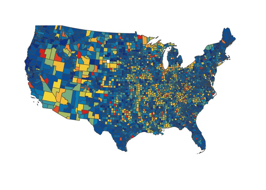
concentrated on node-level characteristics such as node degree [Hol04, MH07, MvdDW13, WKB13].
For instance, models can be used to explore the impact of vaccination strategies that target highly
connected nodes, or various different approaches to contact tracing [Hol04, MH07, MvdDW13,
WKB13].
    Earlier network modelling efforts focused on strategies for node-level characteristics because
data on the structure of entire contact networks was once rare. However, such data is becoming
increasingly available, making it possible to address strategies that target the larger-scale features
of network structure such as how connected communities are to one another. It has been shown
in simulated networks that vaccination targeted at individuals that bridge different communities
in the network are more effective than targeting individuals with high node degree [SJ10]. These
approaches detect important nodes and edges based on edge-betweenness measures. In particular,
edge-betweenness is a measure of the influence an edge has over a diffusion process through
the network (e.g., spread of infectious diseases). A classical example is that of shortest-path
betweenness, which quantifies edge importance based on the assumption that information spreads
only along shortest paths. However, it has been noted [SJ10] that this approach can overlook
important connections in a network. For example, in Figure 1a we see that shortest-path
betweenness only recognizes the shorter “bridge” in the middle, while completely neglecting
the two longer, but still highly influential, side bridges. Random walk betweenness [New05]

    (a) Shortest-path        (b) Current-flow              (c) λ = 1               (d) λ = 2/5

Figure 1: Edge-betweenness: color intensities and edge widths are chosen to reflect relative
magnitude of betweenness measures.

fixes this problem of shortest-path betweenness by assuming that information spreads along
random paths in the network while giving more weight to shorter paths. It is also named
current-flow betweenness [BF05] due to the relation to network electrical current flows. Figure 1b
shows that edge-betweenness that takes into account all possible walks captures the relative
importance of all bridges. However, we note that human movement in large networks tends to
be local [LLDM09, JBP+ 15]. Thus, containing the spread of infectious diseases usually requires
identification and control of contact bottlenecks at a local scale rather than global. For example,
cutting off all three bridges in Figure 1b would be terribly ineffective at slowing down the disease
spread, if there was at least one infectious node in each of the two “square” clusters.
    In this paper we develop a new edge-betweenness measure that we call λ-local flow betweenness,
which is based purely on local diffusion in the network and offers a very flexible and localized
quantification of edge importance. More precisely, when λ is small, λ-local flow betweenness
tends to detect locally important edges as opposed to global bottlenecks that have little influence
on local structure or processes. For example, Figure 1c shows that when λ = 1, it detects the
same global bottlenecks as found by current-flow betweenness, but when we shrink λ = 2/5, it
detects locally important bottlenecks within each block as shown in Figure 1d. Removing these
bottlenecks would reduce disease transmission even if the infection is initially present in both sides.
The proposed definition of edge-betweenness is based on p-norm flow diffusion [YWF20]. This
diffusion is defined as a convex optimization problem that models the phenomenon of diffusing
mass from a given node to nearby nodes that have non-zero capacities. More details are given
in Section 2. The origin of p-norm flow diffusion is in local graph clustering methods. Because
of this, the proposed edge-betweenness method induces locality and clustering biases, which we
discuss in Sub-section 2.1. These inductive biases are crucial to the good performance of the
proposed methods. Details are provided in Section 3.
    We demonstrate that λ-local flow betweenness gives rise to better intervention strategies
on all real datasets that we tested, and we discuss in detail why it is a more suitable measure
for identifying disease transmission bottlenecks. We conduct exhaustive simulations and the
                                                  2
conclusions we draw from all experiments are consistent.

2       Network centrality based on local diffusion
In this section we define λ-local flow betweenness and determine its computational complexity.
λ-local flow betweenness relies on p-norm flow diffusion [YWF20], which is used to solve the local
graph clustering problem [FGM17]. There exist spectral [ST13, ACL06, ZLM13, AP09, FRKS+ 17]
and combinatorial [AL08, OZ14, FLGM20, FGM17, WFH+ 17] local graph clustering methods.
However, p-norm flow diffusion is as simple and as fast as spectral methods, but it has better
conductance guarantees in theory and in practice. Moreover, p-norm diffusion requires less
parameter tuning than combinatorial methods. For these reasons, we use it to define our
edge-betweenness.
    Given an undirected graph G = (V, E) and signed incidence matrix B 1 using arbitrary
orientation, we follow [YWF20] and define a diffusion process on G as the following convex
optimization problem:

                              minimize kf kp      subject to B > f + ∆ ≤ T,                                   (1)

where ∆, T ∈ R|V | specify the amount of initial mass and sink capacity at each node, respectively,
and f ∈ R|E| are edge flow variables. The vector B > f + ∆ gives the amount of final mass at each
node if we start with initial mass ∆ on nodes and send the mass around according to flow routing
f , and we call a flow feasible if the final mass at each node is at most its capacity. The objective
of (1) is to find a feasible flow fp∗ having the minimum p-norm2 . Naturally, in a diffusion we start
with ∆ having high density, i.e., there is a large amount of initial mass concentrated on a small
set of nodes, and the sink capacities enforce we spread the mass to get lower density.
     To take into account all relevant diffusion processes that start from arbitrary nodes and
arbitrary sink capacities, we consider ∆ and T in (1) as random variables following a probability
distribution P, under which its expected optimal objective value is finite. For p ∈ (1, ∞), we
define, in the most general sense, the p-norm flow edge-betweenness for an edge e as

                                       Bp (e; P) := E(∆,T )∼P [|fp∗ (e)|].                                    (2)

Of course, the specific inductive biases of p-norm flow edge-betweenness depend on the distribution
P. For example, let UV denote the discrete uniform distribution on the set of one-hot vectors
{1v : v ∈ V }, then one obtains the current-flow betweenness as a special case:

Theorem 1. For an edge e ∈ E, the current-flow betweenness [BF05] cCB (e) normalized by
1/|V |2 satisfies cCB (e) = B2 (e; UV × UV ) = E∆∼UV ,T ∼UV [|f2∗ (e)|].

2.1      Inductive Biases of λ-local flow betweenness
                                                                                                            d
In order to introduce locality and clustering bias in (2), we let ∆ ∼ UV and fix T =                     λ·vol(G)
where d is the degree vector, vol(G) equals the sum of degrees of all nodes in G, and λ ∈ (0, 1).
We call the resulting specialized p-norm flow edge-betweenness as λ-local flow betweenness, as
the locality of edge flows is controlled by λ, which we state formally in the following.
                                                                  d
Theorem 2 (adapted to our problem from [YWF20]). For T = λ·vol(G)      and any fixed realization
∆ = 1v , the number of edges with nonzero flow crossing them is bounded by kfp∗ k0 < 2λ|E|.

   When p = 2, for any fixed ∆ and T , one can compute f2∗ up to -accuracy in time
O(λ|E|d¯2 log 1 ) where d¯ < maxi∈V di [YWF20]. Therefore, λ-local flow betweenness for all
edges can be computed in time O(λ|V ||E|d¯2 log 1 ). For sparse networks when d¯ is constant, if
    1
    |E| × |V | matrix where the row of edge (u, v) has two non-zero entries, -1 at column u and 1 at column v.
    2                                                ∗
    In general, we use subscripts p, ∆, T and write fp,∆,T to indicate the dependence of optimal solution to input
parameters. We drop ∆, T from the subscript when they are clear from context and simply write fp∗ .

                                                        3
we set λ = O(1/|V |) = O(1/|E|), then the computation time reduces to O(|V | log 1 ). Note that
small λ is what we rely on to detect local contact bottlenecks. In Section 3 we demonstrate that
computing λ-local flow betweenness can be several orders of magnitude faster than computing
shortest-path or current-flow betweenness, while the intervention strategies based on it achieve
better disease containment.
Besides locality, one can show that fp∗ induces a strong local graph clustering bias in sparse
networks for appropriately chosen λ. This local graph clustering bias will play a crucial role in
our experiment. Formally, we quantify how “well-knit” a cluster is by measuring its conductance3 .
Theorem 3 (adapted to our problem from [YWF20]). Fix p ∈ (1, ∞), T = d
λ·vol(G) , and ∆ = 1v
for some node v. The optimal solution to the dual of problem (1) gives a cluster C̃ such that
the conductance φ(C̃) ≤ O(α · φ(C)1−1/p ) holds simultaneously for any subset C containing v,
where α = O( λvol(G)
dv ) and dv is the degree of v. In particular, in sparse graphs when we set
1
λ = O( vol(G) ), the guarantee becomes φ(C̃) ≤ O(φ(C)1−1/p ).
3 Experiments
We compare the effectiveness of interventions for the control of COVID-19 transmission that target
edges4 meeting certain criteria, based on λ-local flow (LF(λ)) betweenness against other network
centrality measures. We compare the following techniques: 1) Uniform Intervention (UI): reduce
all contacts (i.e., edge weights) by a fixed amount, 2) High Degree (HD) intervention: reduce
only the contacts of high degree nodes; and two state-of-the-art betweenness measures, 3) and 4)
Shortest-Path (SP) and Current-Flow (CF) interventions: reduce important contacts recognized
by SP and CF betweenness, respectively. In the past, SP and CF betweenness have been applied
to wide range of problems including cancer diagnosis [Ram17], immunization modelling [SJ10],
power grid contingency analysis [JHC+ 10], terrorist networks analysis [CKS02]. Hence, they are
ideal candidates for comparison purposes. We use two SEIR network models to predict how
COVID-19 infections will spread: 1) an ordinary differential equation (ODE) model where each
node corresponds to a population in which an SEIR epidemic is occurring that can spread between
nodes according to the network’s adjacency matrix, 2) an agent-based model where each node
corresponds to a person, and the infection is transmitted from one node to the next with a certain
probability per timestep. Details about the models and their parameter tuning are given in the
supplementary material. We present the most informative figures in this section. Additional
figures appear in the supplementary.
3.1 Datasets
FB-county network [BCK+ 18, BB18]. This Facebook social network consists of 3142 counties
(nodes). Two counties are connected with an edge if there exists strong social interaction between
them as measured by Facebook interactions.
Wi-Fi hotspots Montreal network [HHE+ 15]. This network consists of 103425 nodes
and 630893 edges. Public WIFI hotspot networks are commonly used as proxies of human contact
networks for studying transmsision of infection across a network of individuals [HHE+ 15, HSB+ 16].
Each individual user is a node and concurrent usage of the same hotspot is an edge.
Portland, Oregon network [EGK+ 04]. This network was generated from time use and
census data for the city of Portland, Oregon. It has been widely used in infectious disease
modelling [EGK+ 04, BaLBB+ 06, WKB13]. The network consists of 1.6 million nodes and 31
million edges. We also make use of a sub-sampled version of this dataset that has 10, 000 nodes
and 199, 168 edges [WKB13].
3 |∂(S)|
The conductance of a subset of nodes S ⊆ V is defined as φ(S) := min{d(S),d(V \S)}
, where ∂(S) = {(u, v) ∈ E :
u ∈ S, v 6∈ S} and d(S) is the sum of degrees of all nodes in S.
4
We reduce targeted contact edge weights by 90%, e.g., physical contact reduction is naturally modelled as
edge weight reduction or deletion. For more experiments under other weight reduction settings, see appendix.
4In Figure 2 we demonstrate the Network Community Profile (NCP), the degree distribution
and epidemic curves without intervention. The NCP captures clustering pattern of a network,
i.e., the lower the NCP is the better. Details about the NCP are given in the supplementary
material. In Figure 2a we demonstrate that the datasets correspond to the three distinct NCP
classifications from [LLDM09, JBP+ 15]. In particular, FB-county has a downward sloping
NCP, i.e., conductance decreases as size increases, Wi-Fi Montreal has roughly flat NCP, i.e.,
conductance does not change much as a function of size, and Portland, Oregon has upward
slopping NCP, i,e, conductance are small at small sizes and increases as the size increases. We
will exploit the NCP structure to define the initially infected nodes in our experiments. In
Figure 2b we illustrate the degree distribution for the datasets. Note that the degree distribution
for Montreal WiFi is heavily concentrated around nodes with degree ≤ 2, which is more than half
of the nodes in the network. This will play crucial role in the analysis of our experiments later on
in this section. In Figure 2c we show the percentage of total active COVID-19 cases (prevelance
of infection) against time (in days). 5
100 0.4
FB-county 0.5 FB-county
Wi-Fi Montreal Wi-Fi Montreal
Total Active Cases
0.3 0.4
Port. Sub.
Percentage of
Port. Sub.
Conductance
Percentage
10 1
0.3 Portland
0.2 Portland
0.2
0.1 0.1
10 2 FB-county Wi-Fi Montreal
Port. Sub. Portland 0.0
0.0 0 25 50 75 100 125 150 0 50 100 150 200
101 102 103 104 105
Size Degree Day
(a) NCPs (b) Degree Distribution (c) Epidemic Curves
Figure 2: NCPs, degree distribution and epidemic curves (without intervention). The NCPs have
been computed using [FLGM19, FGM18] based on the original paper [LLDM09]. The markers in
the NCPs in Figure 2a correspond to clusters that we used to initialize the epidemic models for
Figure 2c.
3.2 Computation time for λ-local flow betweenness
The time required for computing LF(λ) betweenness depends linearly on λ. If the network
is sparse and λ is proportional to 1/|V |, then computing LF(λ) to accuracy can be done in
O(|V | log 1 ) time. For comparison, the computation time is at least O(|V |2 ) for SP betweenness
and O(|V |2 log |V |) for CF betweenness on sparse unweighted graphs6 . In Figure 3 we compare
the empirical computation times for SP, CF, and LF(λ) betweenness on FB-county, Port. Sub.,
and Wi-Fi Montreal networks. All computations are carried out on a personal laptop with 32GB
RAM and 2.9 GHz 6-Core Intel Core i9. We used NetworkX [HSS08] for computing SP and
CF and implemented LF(λ) computation in Julia. Observe that as λ becomes larger and LF(λ)
becomes more global, the time for computing LF(λ) is similar to that of SP or CF. On the other
hand, as λ becomes smaller, computing LF(λ) gets several orders of magnitudes faster. This is
crucial for scaling up our method to huge networks. For example, LF(λ) is the only betweenness
measure we are able to compute for the full Portland network.
5
The curve for FB-county is very different from the other datasets because the data represent a nationwide
geographic region and it takes a longer amount of time for the infection to spread from the Northeastern states to
the rest of the country. This is also the reason that for FB-county the curves have multiple peaks, since there
are multiple outbreaks in multiple cities as the disease progresses. In contrast, the other datasets correspond to
outbreaks in a single urban centre that tend to unfold over weeks instead of months.
6
For arbitrary unweighted graphs, the time is O(|V ||E|) for SP betweenness [Bra01] and
O (I(|V |) + |V ||E| log |V |) for CF betweenness [BF05], where I(n) is the time to invert an n × n matrix.
5(a) FB-county (b) Port. Sub-sampled (c) Wi-Fi Montreal
Figure 3: Comp. time for LF(λ) betweenness. CF is omitted in (c) because it takes too long to
finish.
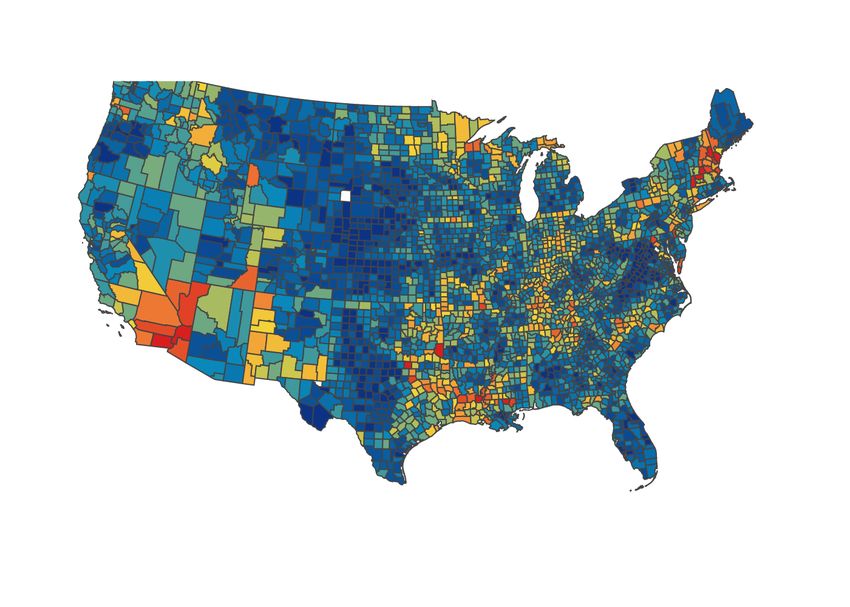
3.3 Experiments for Facebook County network
We apply the ODE model to simulate the spread of COVID-19 on the FB-county network, since
each node represents an entire county population. We assume that all county populations are
initially susceptible and we pick infected counties for which we initialize 0.1% of the county
population as infectious. We use three different ways to select initially infected counties to account
for variations in where outbreaks could have started: (i) populated cosmopolitan cities (e.g.,
New York, Los Angeles), (ii) a tightly-knit cluster of 67 densely connected counties, highlighted
in Figure 4a and also captured by the green star on the NCP in Figure 2a, and (iii) a random
selection of 1% of all counties.
Figure 4b and 4c demonstrate the predicted epidemic curves and the final outbreak sizes during
the epidemic under different levels of intervention for each method, for scenario (iii). (Results
are similar for scenario (i) and (ii), see supplementary material.) Note that the epidemic curve
using LF(λ) intervention starts late, ends earlier, and has the lowest epidemic peak compared to
the interventions based on SP or CF betweenness. Our results also show that for all three initial
conditions and at all levels of intervention, LF(λ) leads to the highest reduction in the epidemic
size.
NI CF NI SP CF LF(1/10)
SP LF(1/50) UI HD LF(1/4) LF(1/50)
0.9
0.07
Total Number of Cases
0.06 0.8
Active Cases
0.05
0.04 0.7
0.03
0.02 0.6
0.01
0.00 0.5
0 50 100 150 200 250 300 10% 20% 30% 40% 50%
Day Percentage of Targeted Edges
(a) Initial cluster of infection (b) Predicted epidemic curves (c) Predicted epidemic final sizes
Figure 4: Simulation results for FB-county. Only four representative epidemic curves at 25%
intervention level are drawn for cleaner visualization: e.g., we removed epidemic curves for HD due
to its poor performance. See supplementary material for all curves and under different scenarios.
To study what makes LF(λ) betweenness a much better indicator for local contact bottlenecks,
we fix the intervention level at 25% of all edges and analyze the resulting networks. In Figure 5
we color each county according to how many edges incident to it have been targeted for contact
reduction. We observe a significant difference in the patterns demonstrated by the three methods.
Intervention based on SP results in scattered targets distributed over the country, whereas CF
emphasizes the central east region, which consists of a large number of concentrated small counties.
Both methods demonstrate a global pattern as being either globally dispersed or globally clustered.
On the other hand, the targets of LF(λ) betweenness form groups of small local clusters that
spread across the country and loosely partition both east and west coasts into several smaller
connected components. This observation is further supported in Figure 6a in which the NCP of
the modified graph based on LF(λ) has much lower conductance when cluster sizes are small.
In Figure 6b we investigate this range by plotting the distribution of clusters of size less than
6100 against conductance. Not surprisingly, the intervened network based on LF(λ) betweenness
contains more well-defined small clusters than the networks obtained from targeting high SP or
CF betweenness, which has a more global focus. Finally, in Figure 6c we measure the percentage
of out-link edges from the initial infected cluster (Figure 4a) that are targeted by different
intervention strategies. Observe that the top 5% edges based on LF(λ) betweenness already
include all edges in the cut of the initial cluster. This explains why the epidemic curve under
LF(λ) starts rising later than others: because all out-link contacts have already been reduced.
Note that LF(λ) is un-supervised, i.e., it is not aware of the initially infected nodes, which
demonstrates that local flow betweenness induces clustering bias, as promised by Theorem 3.
(a) Shortest-path (b) Current-flow (c) 1/50-Local flow
Figure 5: Distribution of target edges reflected by county-level colors: red means most incident
edges are reduced (in edge weights), dark blue means few incident edges are reduced (in edge
weights).
Percentage of Cuts Targeted
NI CF 100%
SP LF(1/50) 80%
Conductance
10 1
60%
40%
SP
10 2 20% CF
0%
LF(1/50)
101 102 103 10% 20% 30% 40% 50%
Size Percentage of Targeted Edges
(a) NCPs, 25% intervention (b) Small clusters, 25% intervention (c) Out-link edges
Figure 6: Network Community Profile (NCP), distribution of small-size clusters (having less than
100 nodes) by conductance, and percentage of targeted out-link edges from the initial cluster of
infection, in the FB-county due to intervention based on different edge-betweenness measures.
3.4 Experiments for Wi-Fi Montreal network
We apply the agent-based SEIR network model to Wi-Fi Montreal, since each node now represents
an individual person. We assign the initial state Susceptible to each person and then pick Infectious
persons in two ways that cover very distinct scenarios: (i) as a group of 120 densely connected
persons captured by the black circle on the NCP in Figure 2a, and (ii) as 0.1% of total population
selected uniformly at random. We simulate the model until all state transitions reach equilibrium.
The results for scenario (i) are shown in Figure 7 (see supplementary material for similar results
for scenario (ii)), where in Figure 7b we also plot the peak of the epidemic curves at different
intervention levels. Observe that in most cases, and in particular when targeting more than 20%
of contact edges, LF(λ) offers both significantly smaller epidemic size and a lower epidemic peak.
CF is omitted for this network due to prohibitive computation time7 . We explain qualitatively
what makes LF(λ) work better than SP. As discussed earlier, more than half of the nodes in
Wi-Fi Montreal have degree one or two (cf. Figure 2b), perhaps because these nodes represent
7
Computing SP betweenness for Wi-Fi Montreal takes more than four days, while computing CF betweenness
would take O(log |V |) more time. As a comparison, computing LF(λ) for λ = 1/50 was done under 10 minutes.
7NI HD NI HD LF(1/4) LF(1/25) NI HD LF(1/4) LF(1/25)
SP LF(1/50) UI SP LF(1/10) LF(1/50) UI SP LF(1/10) LF(1/50)
Maximum Daily Total Active Cases
0.9
0.5
Total Number of Cases
0.5
0.8
0.4
Active Cases
0.4 0.7
0.3
0.2 0.3 0.6
0.1 0.5
0.2
0.0 0.4
0 10 20 30 40 50 10% 20% 30% 40% 50% 10% 20% 30% 40% 50%
Day Percentage of Targeted Edges Percentage of Targeted Edges
(a) Predicted epidemic curves (b) Predicted epidemic peaks (c) Predicted epidemic sizes
Figure 7: Simulation results for Wi-Fi Montreal. Only four representative epidemic curves (at
25% intervention level) are drawn for cleaner visualization. See supplementary for all curves and
under different scenarios. The fluctuations in NI in (b) are due to probabilistic state transitions.
visitors. Hence, this network presents an extreme case where disconnecting all those small degree
nodes could be a trivial yet effective solution. On the other hand, partitioning the entire graph
into groups of clusters may not be as effective as it is for FB-county. In Figure 8 we demonstrate
that LF(λ) captures the degree irregularity in Wi-Fi Montreal and exploits this local information
(i.e., many nodes have low degree). In particular, Figure 8a shows that intervention based on
LF(λ) does not necessarily generate more small clusters when the underlying graph has too many
degree-one nodes. This is supported by Figure 8b where we see that the distribution of clusters
of all sizes in the modified networks are similar. On the other hand, as shown in Figure 8c, where
we measure how many singleton nodes are there if we were to remove all targeted edges, we notice
that LF(λ) separates far more singletons than SP does, thanks to its locality bias. The flexibility
of incorporating local information (or going global if necessary, by controlling the value of λ) is
what makes LF(λ) versatile and effective.
80%
Percentage of Singletons
60%
Conductance
10 1
40%
20%
10 2 SP
NI SP LF(1/50) LF(1/50)
0%
101 102 103 104 10% 20% 30% 40% 50%
Size Percentage of Targeted Edges
(a) NCPs, 25% intervention (b) Cluster dist., 25% intervention (c) Singletons after intervention
Figure 8: Locality bias of LF(λ) for Wi-Fi Montreal is illustrated by the dramatic difference in
(c).
3.5 Experiments for Portland, Oregon
We apply the agent-based model on both sub-sampled and full Portland contact networks. The
sub-sampled network (Port. Sub.) is used first because the computation of both SP and CF
betweenness measures do not scale to the full Portland dataset. We use Port. Sub. for comparison
among different intervention methods and full Portland to demonstrate the effectiveness of LF(λ)
after scaling it up for large networks. We consider two initialization techniques for the model.
First, we use well-connected clusters illustrated by the purple square and the blue diamond on the
NCP in Figure 2a. Second, we select randomly 0.1% nodes from the entire population. For both
datasets, the simulation results for both cluster and random initialization are shown in Figure 9.
Observe that the results from different initialization schemes are very similar. In both scenarios,
the smaller the λ, the smaller the total epidemic size. On the other hand, there is a trade-off
between epidemic peak and epidemic size: on Port. Sub., λ = 1/50 gives the most reduction in
epidemic size, whereas a slightly larger λ = 1/10 offers less reduction in total cases but gives a
flatter epidemic curve (lower peak).
8NI HD CF LF(1/10) NI HD CF LF(1/10) NI HD CF LF(1/10)
UI SP LF(1/4) LF(1/50) UI SP LF(1/4) LF(1/50) UI SP LF(1/4) LF(1/50)
Maximum Daily Total Active Cases
Maximum Daily Total Active Cases
NI HD CF LF(1/10)
UI SP LF(1/4) LF(1/50) 0.90
0.40 0.40 0.90
Total Number of Cases
0.85
Total Number of Cases
0.35 0.35 0.85
0.30 0.80
0.30 0.80
0.25 0.75
0.25
0.75
0.20 0.20 0.70
0.70
0.15 0.15 0.65
10% 20% 30% 40% 50% 10% 20% 30% 40% 50% 0.65 10% 20% 30% 40% 50%
Percentage of Targeted Edges Percentage of Targeted Edges 10% 20% 30% 40% 50% Percentage of Targeted Edges
Percentage of Targeted Edges
(a) Epi. peaks, cluster (b) Epi. peaks, random (d) Epi. sizes, random
(c) Epi. sizes, cluster init.
init. init. init.
NI HD NI HD NI HD
UI LF(1/1000) UI LF(1/1000) UI LF(1/1000)
Maximum Daily Total Active Cases
Maximum Daily Total Active Cases
NI HD
0.50 0.50 UI LF(1/1000) 0.90
0.90
Total Number of Cases
0.85
0.45
Total Number of Cases
0.45 0.85
0.80
0.40 0.40 0.80
0.75
0.35 0.75
0.35 0.70
0.70
0.30 0.65
0.30
0.65
0.60
10% 20% 30% 40% 50% 10% 20% 30% 40% 50% 0.60 10% 20% 30% 40% 50%
Percentage of Targeted Edges Percentage of Targeted Edges 10% 20% 30% 40% 50% Percentage of Targeted Edges
Percentage of Targeted Edges
(e) Epi. peaks, cluster (f) Epi. peaks, random (h) Epi. sizes, random
(g) Epi. sizes, cluster init.
init. init. init.
Figure 9: Simulation results for Port. Sub. (9a through 9d) and full Portland (9e through 9f). For
Portland we used λ = 1/1000 for scalability. We average over 50 trials for random initialization.
0.30 NI NI
0.25 SP 0.3 LF(1/1000)
CF
Conductance
Conductance
10 1
Percentage
Percentage
0.20
0.15
LF(1/50) 10 1 0.2
NI
10 2 SP 0.10 0.1
CF 0.05 NI
LF(1/50) LF(1/1000)
101 102 103 0.00 0 25 50 75 100 125 150 10 2
101 102 103 104 105 0.0 0 25 50 75 100 125 150
Size Degree Size Degree
(a) NCPs, Port. Sub. (b) Deg. dist., Port. Sub. (c) NCPs, Portland (d) Deg. dist., Portland
Figure 10: NCP and degree distribution for modified Port. Sub. and full Portland networks.
For Port. Sub., all three methods produce similar NCPs when cluster sizes are more than
30 as shown in Figure 9a. So NCP does not explain why LF(λ) leads to the most reduction in
epidemic size. We further investigate the degree distributions in Figure 9b. Notice that more than
30% of all nodes in the LF(λ) intervention have degrees close to 0, which is more than double
the amount created from SP or CF. This large amount of almost-isolated nodes (as they have
degrees close to 0) makes it very difficult for an epidemic to spread across the entire population,
and explains why intervention strategies based on LF(λ) leads to the mildest outbreak in terms
of total infection. It also reveals that LF(λ) offers a better utilization of “budget” in the sense
that most efforts in contact reduction are spent to create and isolate low degree nodes. Finally,
for the full Portland network, while Figure 10c shows that there is a small difference in NCP,
such difference is not as significant as it is demonstrated on the Facebook County network, and
the major benefit of using LF(λ) on the full network still lies in the large amount of low degree
nodes it created, as we show in Figure 10d.
4 Conclusion
Infection control methods that target features of network structure instead of features of individual
nodes are increasingly feasible as empirical data on full contact networks becomes more abundant.
At the same time, our network algorithms continue to improve. As we show here, λ local flow
betweenness is orders of magnitude faster than competing methods, and physical distancing
interventions based on λ local flow betweenness mitigate a simulated COVID-19 epidemic on
realistic contact networks more effectively than other state-of-the-art approaches.
9Potential Broader Impact
Large-scale pandemic interventions like school and workplace closure and other forms of physical
(social) distancing can have enormous social and economic impacts. Highly optimized interventions
that target key features of contact network architecture show promise to significantly reduce
epidemic spread with minimal impact on the population, relative to “blunt instruments” like
lockdown that impact the entire network. Our paper introduces a very fast method that can
identify key network features and reduces COVID-19 spread more than competing state-of-the-art
methods. However, implementing these methods in real time during a real-world epidemic would
likely require large-scale digital monitoring of the population, which has negative implications for
invasion of privacy and data protection.
Acknowledgements
The authors are grateful to Thomas Hladish for providing the Montreal WiFi network and to
David F. Gleich for pointing to the Facebook County network. Kimon Fountoulakis would like to
acknowledge NSERC for providing partial support for this work.
References
[ACL06] R. Andersen, F. Chung, and K. Lang. Local graph partitioning using pagerank
vectors. FOCS ’06 Proceedings of the 47th Annual IEEE Symposium on Foundations
of Computer Science, pages 475–486, 2006.
[AEY+ 20] S. C Anderson, A. M Edwards, M. Yerlanov, N. Mulberry, J. Stockdale, S. A
Iyaniwura, R. C Falcao, M. C Otterstatter, M. A Irvine, N. Z Janjua, et al.
Estimating the impact of covid-19 control measures using a bayesian model of
physical distancing. medRxiv, 2020.
[AL08] R. Andersen and K. J. Lang. An algorithm for improving graph partitions. Pro-
ceedings of the nineteenth annual ACM-SIAM symposium on Discrete algorithms,
pages 651–660, 2008.
[AM92] R. M. Anderson and R. M. May. Infectious diseases of humans: dynamics and
control. Oxford university press, 1992.
[AMCyP+ 20] A. Aleta, D. Martin-Corral, A. P. y Piontti, M. Ajelli, M. Litvinova, M. Chinazzi,
N. E Dean, E. M Halloran, I. M Longini, S. Merler, et al. Modeling the impact of
social distancing, testing, contact tracing and household quarantine on second-wave
scenarios of the covid-19 epidemic. medRxiv, 2020.
[AP09] R. Andersen and T. Peres. Finding sparse cuts locally using evolving sets. In
STOC 2009, pages 235–244, 2009.
[BaLBB+ 06] K Bisset, K. Atkins andC. L Barrett, R Beckman, S. Eubank, A. Marathe,
M. Marathe, HS Mortveit, P. Stretz, and VA Kumar. Synthetic data products
for societal infrastructures and proto-populations: Data set 1.0. Technical report,
TR-06-006, Network Dynamics and Simulation, 2006.
[Bau05] C. T Bauch. The spread of infectious diseases in spatially structured populations:
an invasory pair approximation. Mathematical Biosciences, 198(2):217–237, 2005.
[BB18] E. Badger and Q. Bui. How connected is your community to everywhere else in
america? The New York Times, 2018.
10[BC12] F. Brauer and C. C. Chavez. Mathematical models in population biology and
epidemiology, volume 2. Springer, 2012.
[BCK+ 18] M. Bailey, R. Cao, T. Kuchler, J. Stroebel, and A. Wong. Social connected-
ness: Measurement, determinants, and effects. Journal of Economic Perspectives,
32(3):259–280, 2018.
[BF05] U. Brandes and D. Fleischer. Centrality measures based on current flow. In
Volker Diekert and Bruno Durand, editors, STACS 2005, pages 533–544, Berlin,
Heidelberg, 2005. Springer Berlin Heidelberg.
[BHR+ 20] P. Block, M. Hoffman, I. J Raabe, J. B. Dowd, C. Rahal, R. Kashyap, and M. C
Mills. Social network-based distancing strategies to flatten the covid 19 curve in a
post-lockdown world. arXiv preprint arXiv:2004.07052, 2020.
[Bra01] U. Brandes. A faster algorithm for betweenness centrality. The Journal of Mathe-
matical Sociology, 25(2):163–177, 2001.
[CDA+ 20] M. Chinazzi, J. T Davis, M. Ajelli, C. Gioannini, M. Litvinova, S. Merler, A. P.
y Piontti, K. Mu, L. Rossi, K. Sun, et al. The effect of travel restrictions on the
spread of the 2019 novel coronavirus (covid-19) outbreak. Science, 368(6489):395–
400, 2020.
[CDS09] R. Connell, P. Dawson, and A. Skvortsov. Comparison of an agent-based model
of disease propagation with the generalised sir epidemic model. Technical report,
Defense Science and Technology Organization Victoria (Australia), 2009.
[CKS02] T. Carpenter, G. Karakostas, and D. Shallcross. Practical issues and algorithms
for analyzing terrorist networks 1. In Proceedings of the Western Simulation
MultiConference, 2002.
[CPS10] C. Castellano and R. Pastor-Satorras. Thresholds for epidemic spreading in
networks. Physical review letters, 105(21):218701, 2010.
[CST+ 20] H. F. Chan, A. Skali, B. Torgler, et al. A global dataset of human mobility.
Technical report, Center for Research in Economics, Management and the Arts
(CREMA), 2020.
[EGK+ 04] S. Eubank, H. Guclu, VS A. Kumar, M. V Marathe, A. Srinivasan, Z. Toroczkai,
and N. Wang. Modelling disease outbreaks in realistic urban social networks.
Nature, 429(6988):180–184, 2004.
[ERBG00] D. JD Earn, P. Rohani, B. M Bolker, and B. T Grenfell. A simple model for
complex dynamical transitions in epidemics. Science, 287(5453):667–670, 2000.
[FGM17] K. Fountoulakis, D. F. Gleich, and M. W. Mahoney. An optimization approach to
locally-biased graph algorithms. Proceedings of the IEEE, 105(2):256–272, 2017.
[FGM18] K. Fountoulakis, D. F. Gleich, and M. W. Mahoney. A short introduction to
local graph clustering methods and software. Technical report, 2018. Preprint:
arXiv:1810.07324.
[Fin03] P. EM Fine. The interval between successive cases of an infectious disease. American
journal of epidemiology, 158(11):1039–1047, 2003.
[FLGM19] K. Fountoulakis, M. Liu, D. Gleich, and M. W. Mahoney. Localgraphclustering
API. https://github.com/kfoynt/LocalGraphClustering, January 2019.
11[FLGM20] K. Fountoulakis, M. Liu, D. F. Gleich, and M. W. Mahoney. Flow-based algorithms
for improving clusters: A unifying framework, software, and performance. Technical
report, 2020. Preprint: arXiv:2004.09608.
[FRKS+ 17] K. Fountoulakis, F. Roosta-Khorasani, J. Shun, X. Cheng, and M. W. Mahoney.
Variational perspective on local graph clustering. Mathematical Programming B,
pages 1–21, 2017.
[GBB+ 06] V. Grimm, U. Berger, F. Bastiansen, S. Eliassen, V. Ginot, J. Giske, J. Goss-
Custard, T. Grand, S. K Heinz, G. Huse, et al. A standard protocol for describing
individual-based and agent-based models. Ecological modelling, 198(1-2):115–126,
2006.
[GBD+ 10] V. Grimm, U. Berger, D. L DeAngelis, J G. Polhill, J. Giske, and S. F Railsback.
The odd protocol: a review and first update. Ecological modelling, 221(23):2760–
2768, 2010.
[HBB+ 20] N. Hoertel, M. Blachier, C. Blanco, M. Olfson, M. Massetti, F. Limosin, and
H. Leleu. Facing the covid-19 epidemic in nyc: a stochastic agent-based model of
various intervention strategies. medRxiv, 2020.
[HD19] J. Hackl and T. Dubernet. Epidemic spreading in urban areas using agent-based
transportation models. Future Internet, 11(4):92, 2019.
[Het00] H. W. Hethcote. The mathematics of infectious diseases. SIAM Review, 42(4):599–
653, 2000.
[HHE+ 15] A. G. Hoen, T. J. Hladish, R. M. Eggo, M Lenczner, J. S. Brownstein, and L. A.
Meyers. Epidemic wave dynamics attributable to urban community structure: A
theoretical characterization of disease transmission in a large network. Journal of
Medical Internet Research, 17(7), 2015.
[HK20] J. Hilton and M. J Keeling. Estimation of country-level basic reproductive ratios
for novel coronavirus (covid-19) using synthetic contact matrices. medRxiv, 2020.
[Hol04] P. Holme. Efficient local strategies for vaccination and network attack. EPL
(Europhysics Letters), 68(6):908, 2004.
[HSB+ 16] J. L Herrera, R. Srinivasan, J. S Brownstein, A. P Galvani, and L. A. Meyers.
Disease surveillance on complex social networks. PLoS computational biology, 12(7),
2016.
[HSS08] A. A. Hagberg, D. A. Schult, and P. J. Swart. Exploring network structure,
dynamics, and function using networkx. In Gaël Varoquaux, Travis Vaught, and
Jarrod Millman, editors, Proceedings of the 7th Python in Science Conference,
pages 11 – 15, Pasadena, CA USA, 2008.
[JBP+ 15] L. G. S. Jeub, P. Balachandran, M. A. Porter, P. J. Mucha, and M. W. Mahoney.
Think locally, act locally: Detection of small, medium-sized, and large communities
in large networks. Physical Review E, 91:012821, 2015.
[JHC+ 10] S. Jin, Z. Huang, Y. Chen, D. Chavarría-Miranda, J. Feo, and P. C. Wong. A novel
application of parallel betweenness centrality to power grid contingency analysis. In
2010 IEEE International Symposium on Parallel Distributed Processing (IPDPS),
pages 1–7, 2010.
[KAB20] V. Karatayev, M. Anand, and C. T Bauch. The far side of the covid-19 epidemic
curve: local re-openings based on globally coordinated triggers may work best.
medRxiv, 2020.
12[KE05] M. J Keeling and K. TD Eames. Networks and epidemic models. Journal of the
Royal Society Interface, 2(4):295–307, 2005.
[KHG+ 20] M. J. Keeling, E. Hill, E. Gorsich, B. Penman, G. Guyver-Fletcher, A. Holmes,
T. Leng, H. McKimm, M. Tamborrino, L. Dyson, et al. Predictions of covid-19
dynamics in the uk: short-term forecasting and analysis of potential exit strategies.
medRxiv, 2020.
[KYG+ 20] M. UG Kraemer, C. Yang, B. Gutierrez, C. Wu, B. Klein, D. M Pigott, P. L. du,
N. R Faria, R. Li, W. P Hanage, et al. The effect of human mobility and control
measures on the covid-19 epidemic in china. Science, 368(6490):493–497, 2020.
[LGWSR20] Y. Liu, A. A Gayle, A. Wilder-Smith, and J. Rocklöv. The reproductive number of
covid-19 is higher compared to sars coronavirus. Journal of travel medicine, 2020.
[LLDM09] J. Leskovec, K.J. Lang, A. Dasgupta, and M.W. Mahoney. Community structure in
large networks: Natural cluster sizes and the absence of large well-defined clusters.
Internet Mathematics, 6(1):29–123, 2009.
[ME06] J. Ma and D. JD Earn. Generality of the final size formula for an epidemic of a
newly invading infectious disease. Bulletin of mathematical biology, 68(3):679–702,
2006.
[MH07] J. C Miller and J. M Hyman. Effective vaccination strategies for realistic social
networks. Physica A: Statistical Mechanics and its Applications, 386(2):780–785,
2007.
[MvdDW13] J. Ma, P v. d. Driessche, and F. H Willeboordse. The importance of contact
network topology for the success of vaccination strategies. Journal of theoretical
biology, 325:12–21, 2013.
[New05] M.E. J. Newman. A measure of betweenness centrality based on random walks.
Social Networks, 27(1):39 – 54, 2005.
[NKY+ 20] M Linton N, T. Kobayashi, Y. Yang, K. Hayashi, A. R Akhmetzhanov, S. Jung,
B. Yuan, R. Kinoshita, and H. Nishiura. Incubation period and other epidemio-
logical characteristics of 2019 novel coronavirus infections with right truncation:
a statistical analysis of publicly available case data. Journal of clinical medicine,
9(2):538, 2020.
[NLA20] H. Nishiura, N. M Linton, and A. R Akhmetzhanov. Serial interval of novel
coronavirus (covid-19) infections. International Journal of Infectious Diseases,
2020.
[OZ14] L. Orecchia and Z. A. Zhu. Flow-based algorithms for local graph clustering. In
Proceedings of the 25th Annual ACM-SIAM Symposium on Discrete Algorithms,
pages 1267–1286, 2014.
[PB09] A. Perisic and C. T Bauch. Social contact networks and disease eradicability under
voluntary vaccination. PLoS Comput Biol, 5(2):e1000280, 2009.
[PBB+ 15] L. Pellis, F. Ball, S. Bansal, K. Eames, T. House, V. Isham, and P. Trapman. Eight
challenges for network epidemic models. Epidemics, 10:58–62, 2015.
[PD09] L. Perez and S. Dragicevic. An agent-based approach for modeling dynamics of
contagious disease spread. International Journal of Health Geographics, 8(1):50,
2009.
13[Ram17] J. Ramasamy. A Betweenness Centrality Guided Clustering Algorithm and Its
Applications to Cancer Diagnosis, pages 35–42. Springer, 01 2017.
[RKW95] D. Rand, M. Keeling, and H. Wilson. Invasion, stability and evolution to criticality
in spatially extended, artificial host—pathogen ecologies. Proceedings of the Royal
Society of London. Series B: Biological Sciences, 259(1354):55–63, 1995.
[RSK20] O. Reich, G. Shalev, and T. Kalvari. Modeling covid-19 on a network: super-
spreaders, testing and containment. medRxiv, 2020.
[SJ10] M. Salathé and J. H. Jones. Dynamics and control of diseases in networks with
community structure. PLOS Computational Biology, 6(4):1–11, 04 2010.
[SRKFM16] J. Shun, F. Roosta-Khorasani, K. Fountoulakis, and M. W. Mahoney. Parallel local
graph clustering. Proceedings of the VLDB Endowment, 9(12):1041–1052, 2016.
[ST13] D. A. Spielman and S. H. Teng. A local clustering algorithm for massive graphs
and its application to nearly linear time graph partitioning. SIAM Journal on
Scientific Computing, 42(1):1–26, 2013.
[TFG20] A. Tuite, D. N Fisman, and A. L Greer. Mathematical modeling of covid-19 trans-
mission and mitigation strategies in the population of ontario, canada. medRxiv,
2020.
[VTD+ 20] A. Vespignani, H. Tian, C. Dye, J. O. Lloyd-Smith, R. M. Eggo, M. Shrestha, S. V.
Scarpino, B. Gutierrez, M. UG. Kraemer, J. Wu, et al. Modelling covid-19. Nature
Reviews Physics, pages 1–3, 2020.
[WFH+ 17] D. Wang, K. Fountoulakis, M. Henzinger, M. W. Mahoney, and S. Rao. Capacity
releasing diffusion for speed and locality. In Proceedings of the 34th International
Conference on Machine Learning, volume 70, pages 3607–2017, 2017.
[WKB13] C. R Wells, E. Y Klein, and C. T Bauch. Policy resistance undermines superspreader
vaccination strategies for influenza. PLoS computational biology, 9(3), 2013.
[YD20] D. Yao and R. Durrett. Epidemics on evolving graphs. arXiv preprint
arXiv:2003.08534, 2020.
[YWF20] S. Yang, D. Wang, and K. Fountoulakis. p-norm flow diffusion for local graph
clustering. In Proceedings of the 37th International Conference on Machine Learning,
2020.
[ZLM13] Z. A. Zhu, S. Lattanzi, and V. S. Mirrokni. A local algorithm for finding well-
connected clusters. In Proceedings of the 30th International Conference on Machine
Learning, pages 396–404, 2013.
14Supplementary material
A SEIR models
Models of infectious disease transmission typically divide the population into compartments based
on their infection status, such as susceptible (S), infectious (I) and removed/recovered (R) [BC12,
AM92]. Individuals move between compartments at certain rates according to assumptions about
transmission and disease progression, and the compartments depend on disease or intervention
being studied. For instance, an SLIR model with a latent (L) compartment accounts for the stage
between being infected and starting to infect others [AMCyP+ 20]. Ordinary differential equations
are often used to model the transmission processes in a large, homogeneously mixing population and
can approximate dynamics adequately for many situations [Het00, TFG20, ERBG00]. For other
applications it may be desirable to account for stochastic effects or contact heterogeneities, in which
case probabilistic models and/or network models are preferable [YD20, KAB20, CDS09, PD09].
Agent-based models are an important subclass where simulated agents evolve according to certain
rules and transitions between states are typically described as a probabilistic process [GBB+ 06],
and are being widely used in the COVID-19 pandemic [HBB+ 20]. These models can simulate
fine-scale individual movement behaviour or epidemiological characteristics [PD09, HD19].
In this paper we use two different types of COVID-19 transmission models. Both assume
an SEIR disease progression in the host where individuals are in one of four mutually exclusive
compartments: susceptible to infection (S), infected but not yet infectious (E), infectious (I), and
removed (R). The first model described below is based on a system of ordinary differential equations
(ODEs) [Het00] while the second is an agent-based model [GBB+ 06, GBD+ 10, WKB13].
A.1 Ordinary Differential Equation SEIR Network Model
Our ODE network SEIR model assumes that the proportion of susceptible, exposed, infectious
and removed individuals in each population evolves according to an SEIR ODE model, and
that transmission between populations occur through a network that connects these populations
at rates determined by the network structure (connectivity and edge weights) of the Facebook
County network. We define the following compartments:
• Si (t): number of susceptible persons at time t in population i,
• Ei (t): number of exposed persons (infected but not yet infectious) at time t in population i,
• Ii (t): number of infectious persons at time t in population i,
• Ri (t): number of removed persons at time t in population i,
• Ni : number of persons in population i (constant),
and the following parameters:
• Aji : number of contacts through which individuals in population j can infect individuals in
population i. Aji captures edge weights in the network of populations,
• β: average transmission rate per unit time per contact,
• σi : average rate per unit time at which an individual transitions from the exposed stage to
the infectious stage, in population i,
• γi : average rate per unit time at which an individual transitions from the infectious stage
to the removed stage, in population i,
15The corresponding ODE SEIR network model is
dSi X Ij
= −β Aji Si
dt Nj
j
dEi X Ij
=β Aji Si − σi Ei
dt Nj
j
dIi
= σi Ei − γi Ii
dt
dRi
= γi Ii .
dt
For our simulations we assume σi = σ and γi = γ for all i.
A.2 Agent Based Model SEIR Network Model
To model infection spread in a network of individuals, we introduce an agent-based network
SEIR simulation model [GBB+ 06, GBD+ 10, WKB13]. An individual can be placed into one of
following four states: (1) Susceptible (can contract the infection given contact with an infected
individual), (2) Exposed (contracted the infection, but not yet infectious), (3) Infectious (with or
without symptoms), and (4) Removed (either dead or obtained immunity and hence cannot infect
others). The number of Susceptible, Exposed, Infectious, Removed, and total individuals can be
denoted as S, E, I, R, N, respectively. When an infectious individual passes the infection to a
susceptible individual, the susceptible agent is activated. The algorithm allows us to keep track
of the Exposed and Infectious agents over time. As the number of activated agents increases so
does the computational expense. We assumed that all edges have the same weight.
The total number of individuals within each of these disease states is given as:
• S(t): number of susceptible persons at time t,
• E(t): number of exposed persons (infected but not yet infectious) at time t,
• I(t): number of infectious persons at time t,
• R(t): number of removed persons at time t,
• N : number of persons in the population (constant),
and the parameters are:
• β: transmission probability along a network edge, per unit time,
• σ: probability that a person transitions from exposed to infectious, per unit time,
• γ: probability that a person transitions from infectious to removed, per unit time,
Each timestep in the discrete-time simulation corresponds to one day. The corresponding algorithm
is as follows
1. Loop over all nodes (each node is a person) for each time step. For each node, the following
may happen
• If a person is in state S, then each infected neighbouring person has a probability β of
infecting him/her, in which case the susceptible person moves from state S → E.
• If a person is in state E, s/he becomes infectious with probability σ and the status
changes from E → I.
• If a person is in state I, s/he recovers with probability γ and the status changes from
I → R.
2. Update status of each person according to the events the person went through.
3. Repeat the steps for desired number of time steps.
16A.3 COVID-19 model parameterization
We set the average duration of the latent period 1/σ = 2.5 days and the average duration of
the infectious period 1/γ = 5 days based on epidemiological data on COVID-19 serial interval
and incubation period [NLA20, NKY+ 20]. (We note that the latent and infectious periods do
not correspond to the incubation period and duration of illness [Fin03].) We assumed a basic
reproduction number R0 = 2.5 for COVID-19 [LGWSR20, HK20]. We use the same values
of σ, γ, and R0 for both models. Calibration of the differential equation SEIR model for the
Facebook County network and the agent-based SEIR model for the Wi-Fi Montreal and Portland
networks required calibrating the value of β. In the agent-based network model, β is simply
the transmission probability per edge per timestep. In the differential equation model, β is the
coefficient of transmission in front of the adjacency matrix Aji . In order to ensure comparability
between these two model outputs, we calibrated their respective β values to obtain the outcome
that 89% of the populationPeventually becomes infected in the absence of any interventions, in
both models (i.e., limt→∞ i Ri /Ni = 0.89). This percentage was based on the SEIR epidemic
final size formula Z = 1 − exp(−ZR0 ) where Z is the final size [ME06], and our assumption that
R0 = 2.5. We modelled edge weight reduction due to interventions by reducing β values on the
targeted edges accordingly.
B Missing proofs
B.1 Proof of Theorem 1
Fix p = 2, ∆ = 1s and T = 1t for some s, t ∈ V . Then the p-norm flow diffusion optimization
problem
minimize kf kp subject to B > f + ∆ ≤ T,
becomes
minimize kf k2 subject to B > f + 1s ≤ 1t ,
or equivalently,
minimize 12 kf k22 subject to B > f + 1s = 1t . (B.1)
where the equality constraint in the above is due to the fact k1s k1 = k1t k1 . Let fst denote
the optimal solution of (B.1). Then by the optimality condition of (B.1), fst satisfies, for some
y ∈ R|V | ,
fst + By = 0, (B.2)
−B fst = 1s − 1t .
>
(B.3)
Pre-multiply both sides of (B.2) by B > , and substitute (B.3), we have
Ly = B > By = −B > fst = 1s − 1t , (B.4)
where L is the Laplacian matrix of G. Notice that (B.4) is exactly the Laplacian linear system
that defines the absolute potentials y of a unique st-current τst (e.g., see Lemma 3 in [BF05]),
where τ (e) = y(u) − y(v) for e = (u, v) ∈ E. Now, the relations between fst and y are given
by (B.3), i.e.,
fst (e) = y(v) − y(u), for e = (u, v) ∈ E.
Therefore fst (e) = −τst (e) for all e. Moreover, if s = t, then simply fst (e) = 0 for all e. It follows
that
1 X 1 X
E∆∼UV ,T ∼UV [|f2∗ (e)|] = |fst (e)| = |τst (e)|,
|V |2 |V |2
s,t∈V s,t∈V,s6=t
which is exactly the current-flow betweenness [BF05] normalized by 1/|V |2 .
17B.2 Proofs of Theorem 2 and Theorem 3
Theorem 2 comes directly from Lemma 1 in [YWF20]. Theorem 3 is a straightforward application
of Theorem 2 in [YWF20] to our setting.
C Network Community Profile
In the seminal papers [LLDM09, JBP+ 15] the authors studied how clustering structure of social
networks changes as the size of the clusters increases. In particular, the NCP [LLDM09, JBP+ 15]
function is defined as:
Φ(k) := min φ(S) subject to: |S| = k.
S⊂V
The NCP function takes as input the size k and asks for the minimum conductance that can
be found in the graph such that the set S has size k. The NCP can be used to calculate the
clustering resolution profile of the network as the size of the set increases. Based on the NCP,
many real-world networks can be classified into three distinct cases according to their “size-resolved
community structure”, (i) the best small communities have lower conductance than the best
large communities (upward slopping NCP), (ii) the best small communities have comparable
conductance to the best medium-sized and large communities (flat NCP), and (iii) the best
small communities have higher conductance than the best large groups (downward slopping
NCP). Computing the NCP function is NP-hard and it cannot be computed exatly, however,
in [LLDM09, JBP+ 15] the authors have shown that it can be approximated (empirically) using
local graph clustering algorithms [FGM17, WFH+ 17, FRKS+ 17, SRKFM16].
D More details about the datasets
FB-county network [BCK+ 18, BB18]. This Facebook social network consists of 3100 counties
(nodes) and 22138 edges. Two counties are connected with an edge if there exists strong social
interaction between them as measured by Facebook interactions. In this report, out of all the
edges we keep only those that correspond to counties less than 500 miles apart. The resulting
graph is still a connected graph. The post-processed graph maintains the structural properties
that are discussed in the original article and paper [BCK+ 18, BB18], that is, social interaction
tends to happen mostly among nearby counties.
Wi-Fi hotspots Montreal network [HHE+ 15]. This is a public WIFI hotspot network
which we interpret as a contact network. WIFI networks are commonly used as proxies of human
contact networks for studying transmsision of infection across a network of individuals [HHE+ 15,
HSB+ 16] This particular network is by Île Sans Fil (ÎSF), a not-for-profit organization established
in 2004 in Montreal, Canada, that operates a system of public internet hotspots. Each individual
user is a node and concurrent usage of the same hotspot is an edge. We use the post-processed
network by [HHE+ 15], which consists of 103425 nodes and 630893 edges.
Portland, Oregon network [EGK+ 04]. This synthetic network was generated from time
use and census data for the city of Portland, Oregon. It has also been widely used in infectious
disease modelling [EGK+ 04, BaLBB+ 06, WKB13]. The full dataset consists of 1.6 million nodes
and 31 million edges. We also make use of a sub-sampled version of this dataset that has 10, 000
nodes and 199, 168 edges [WKB13]. The reason that we sub-sample the original network is
because the SP and CF betweenness methods do not scale to the initial network.
E Complete simulation results for intervention strategies with
90% weight reduction on targeted edges
In this section we show complete simulation results for all four networks: Facebook County, Wi-Fi
Montreal, Portland Sub-sampled, and Portland, including the plots that are omitted in the main
18You can also read