Model-based projections for COVID-19 outbreak size and student-days lost to closure in Ontario childcare centres and primary schools
←
→
Page content transcription
If your browser does not render page correctly, please read the page content below
Model-based projections for COVID-19 outbreak size
and student-days lost to closure in Ontario childcare
centres and primary schools
Brendon Phillips1,2 , Dillon T. Browne2 , Madhur Anand3 , and Chris T. Bauch1,*
1 Department  of Applied Mathematics, University of Waterloo, Waterloo, Ontario, Canada
2 Department  of Psychology, University of Waterloo, Waterloo, Ontario, Canada
3 School of Environmental Sciences, University of Guelph, Guelph, Ontario, Canada
* cbauch@uwaterloo.ca

ABSTRACT

The disruption of professional childcare has emerged as a substantial collateral consequence of the public health precautions
related to COVID-19. Increasingly, it is becoming clear that childcare centers must be (at least partially) operational in order to
further mitigate the socially debilitating challenges related to pandemic induced closures. However, proposals to safely reopen
childcare while limiting COVID-19 outbreaks remain understudied, and there is a pressing need for evidence-based scrutiny of
the plans that are being proposed. Thus, in order to support safe childcare reopening procedures, the present study employed
an agent-based modeling approach to generate predictions surrounding risk of COVID-19 infection and student-days lost
within a hypothetical childcare center hosting 50 children and educators. Based on existing proposals for childcare and school
reopening in Ontario, Canada, six distinct room configurations were evaluated that varied in terms of child-to-educator ratio
(15:2, 8:2, 7:3), and family clustering (siblings together vs. random assignment). The results for the 15:2 random assignment
configuration are relevant to early childhood education in Ontario primary schools, which require two educators per classroom.
High versus low transmission rates were also contrasted, keeping with the putative benefit of infection control measures within
centers, yielding a total of 12 distinct scenarios. Simulations revealed that the 7:3 siblings together configuration demonstrated
the lowest risk, whereas centres hosting classrooms with more children (15:2) experienced 3 to 5 times as many COVID-19
cases. Across scenarios, having less students per class and grouping siblings together almost always results in significantly
lower peaks for number of active infected and infectious cases in the institution. Importantly, the total student-days lost to
classroom closure were between 5 and 8 times higher in the 15:2 ratios than for 8:2 or 7:3. These results suggest that current
proposals for childcare reopening could be enhanced for safety by considering lower ratios and sibling groupings.

1 Introduction
As nations around the world grapple with the psychosocial, civic, and economic ramifications of social distancing guidelines, the
critical need for widely-available Early Childhood Education (or colloquially, “childcare”) services have, once again, reached
the top of policy agendas1, 2 . Whether arguments are centered on human capital (i.e., “children benefit from high-quality,
licensed educational environments, and have the right to access such care”) or the economy (i.e., “parents need childcare in
order to work, and the economy needs workers to thrive”), the conclusion is largely the same: childcare centers are re-opening,
at least in some capacity, and this is taking place before a vaccine or herd immunity can mitigate potential COVID-19 spread.
Outbreaks of COVID-19 in emergency childcare centers and schools have already been observed3 , causing great concern as
governments struggle to balance “flattening the curve” and preventing second waves with other pandemic-related sequelae,
such as the mental well-being of children and families, access to education and economic disruption.
     Governments and childcare providers are tirelessly planning the operations of centers, with great efforts to follow public
health guidelines for reducing COVID-19 contagion4 . However, these guidelines, which will result in significantly altered
operational configurations of childcare centers and substantial cost increases, have yet to be rigorously examined. Moreover,
discussions of childcare are presently eclipsed by general discussion of “school” reopening5 . That being said, for many parents,
the viability of the school-day emerges from before and after school programming that ensures adequate coverage throughout
parents’ work schedules. Yet, reopening plans often fail to mention the critical interplay between school and childcare, even
though many childcare centers operate within local schools6 . Consequently, a model that comprehensively examines the
multifaceted considerations surrounding childcare operations may help inform policy and planning. As such, the purpose of the
present investigation is to develop an agent-based model that explores and elucidates the multiple interacting factors that could
impact potential COVID-19 spread in school-based childcare centers.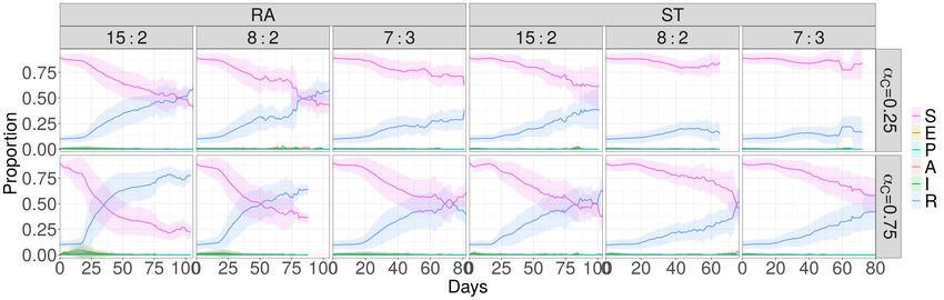
In Ontario, Canada (the authors’ jurisdiction), childcare centers were permitted to reopen on June 12, 2020, provided centers
limit groupings (e.g., classrooms) to a maximum of 10 individuals (educators and children, inclusive)7 . Additionally, all centers
had to come up with a plan for daily screening of incoming persons, thorough cleaning of rooms before and during operations,
removal of toys that pose risk of spreading germs, allowing only essential visitors, physical distancing at pick-up and drop-off,
and a contingency plan for responding should anyone be exposed to the virus (e.g., closing a classroom or center for a period of
time). Further school-specific recommendations have been recently outlined by The Toronto Hospital for Sick Children6 , which
include specific guidelines for screening, hand hygiene, physical distancing, cleaning, ventilation, and masking. While this
influential report has become the guiding framework for school reopening in Ontario, there remains no discussion of childcare
operations in relation to COVID-19 spread.
    Simulation models of infectious disease spread have been widely applied during the COVID-19 pandemic, as in previous
pandemics8, 9 . Modelling is used to determine how quickly the pathogen can spread10 , how easily it may be contained11 , and the
relative effectiveness of different containment strategies12, 13 . Sensitivity analysis is crucial to assess whether model predictions
are robust to uncertainties in data14 , which is particularly important during a pandemic caused by a novel emerging pathogen
like SARS-CoV-2 (the virus that causes COVID-19). Agent-based models are particularly well-suited to situations where a
highly granular description of the population is desirable and where random effects (stochasticity) is important. Such models
have been previously applied in both pandemic and non-pandemic situations15–17 , and is our choice of modelling methodology
in the present work focusing on COVID-19 transmission in schools and homes.
    Below, the methodological approach, results, and interpretation of the present modelling exercise will be illustrated. In the
Methods section, the rationale and parameterization of the model is specified in detail. In the Results section, the performance
of the model under different assumptions is showcased. Lastly, the discussion will provide a review and interpretation of this
study, including any limitations and future suggestions for research.

2 Model Overview
A detailed description of the model structure, assumptions and parameterization appears in the Methods section. We developed
an agent-based model of SARS-CoV-2 transmission (hereafter, COVID-19) in a population structured into households and
classrooms, as might represent a childcare setting or a small school (Figure 1). Individuals were categorized into either
child or adult, and contacts between these groups were parameterized based on contact matrices estimated for the Canadian
setting. Household sizes were determined from Canadian demographic data. Classroom sizes and teacher-student ratios were
determined according to the scenario being studied. Six distinct room occupancy scenarios were tested. In the case of modelling
a childcare centre, the two child-care provider ratios tested were 8:2 and 7:3, with a maximum class size of 10 representative
of the smaller enrollment at childcare centres. For the school scenario, we used a student-teacher ratio 15:2, giving a total
class size of 17. This could represent smaller classes at the primary level, including kindergarten classes which often have two
teachers in Ontario. This could also represent some childcare settings.
    Along with class size, we also consider class composition. Individuals may spread the infection to their household members
each day, so effective contacts and interaction in the classroom may result in qualitatively different spreading patterns. As such,
children in this model can be assigned to classrooms either randomly (RA) or by grouping siblings (or otherwise cohabiting
students) together (ST) in an attempt to reduce COVID-19 transmission.
    COVID-19 could be transmitted in households, classrooms or in common areas of the school, all of which were treated as
homogeneously mixing on account of evidence for aerosolized routes of infection. Individuals were also subject to a constant
risk of infection from other sources, such as shopping centres. Figure 2 shows the progression of the illness experienced by each
individual in the model. In each day, susceptible (S) individuals exposed to the disease via community spread or interaction with
infectious individuals (those with disease statuses P, A and I) become exposed (E), while previously exposed agents become
presymptomatic (P) with probability δ . Presymptomatic agents develop an infection in each day with probability δ , where they
can either become symptomatically infected (I) with probability η or asymptomatically infected (A) with probability 1 − η. If a
symptomatic individuals appears in a classroom, that classroom is closed for 14 days, although other classrooms in the same
school may remain open.
    Finally, we considered both a high transmission rate scenario, using epidemiological data from the early days of the
COVID-19 pandemic, and a low transmission rate scenario, representing a setting with highly effective infection control through
consistent use of high-effectiveness masks, social distancing, and disinfection protocols (see Methods section for details). In
total the permutations on student-teacher ratios, transmission rate assumptions, and siblings versus non-sibling groupings
yielded twelve scenarios (Table 1).

                                                                                                                                2/26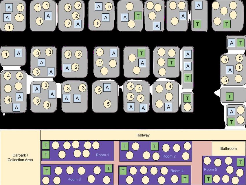
Figure 1. Schematic representation of model population. ‘A’ represents adult, ‘T’ represents teacher, and circles represent
children. Grey rectangles represent houses and the school is represented at the bottom of the figure. Numbers exemplify
possible assignments of children in households to classrooms.

                                                                                   I
                                                                    σ ·η                       γI

                              λ∗                    δ
                   S                     E                    P                                          R

                                                               σ · (1 − η)                          γA

                                                                                  A
Figure 2. Diagram showing the SEPAIR infection progression for each agent in the simulation (see Methods for definitions of
parameters).

3 Results
3.1 Features of the initial stages of the outbreak
The basic reproduction number R0 is the average number of secondary infections produced by a single infected person in
an otherwise susceptible population18 . When there is pre-existing immunity, as we suppose here, we study the effective
reproduction number Re –the average number of secondary infections produced by a single infected person in a population with
some pre-existing immunity. Figure 3 shows the estimated Re and mean population size (childcare centre plus all associated
households) over the course of each simulation, computed by tracking the number of secondary infections produced by a single
primary case. The Re values in the simulation range from 1.5 to 3 on average, depending on the scenario. As expected, these Re
values–which track COVID-19 transmission only in classrooms and households–are generally lower than the typical range
of values between 2 to 3 reported in the literature, which are measured for COVID-19 transmission in all settings, including
workplaces and other sources of community spread19–21 .
    There is little correlation between mean population size (Fig. 3, line), number of households (not shown) and the corre-
sponding R estimate (Fig. 3, bars), leaving only the number of children per classroom responsible for the gross decreasing

                                                                                                                         3/26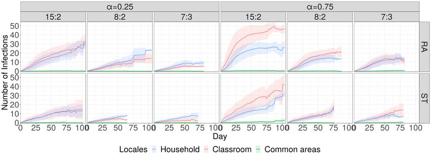
siblings togethern (ST)
15:2 student to teacher ratio
random allocation (RA)
siblings together
High transmission 8:2 student to teacher ratio
random allocation
siblings together
7:3 student to teacher ratio
random allocation
siblings togethern
15:2 student to teacher ratio
random allocation
siblings together
Low transmission 8:2 student to teacher ratio
random allocation
siblings together
7:3 student to teacher ratio
random allocation
Table 1. Twelve Scenarios Evaluated
Figure 3. Bar chart showing the effective reproduction number Re in the entire population (with error bars denoting one
standard deviation), with a line plot showing the mean population size. Both low and high transmission scenarios are shown.
trend in R in both high (α = 0.75) and low (α = 0.25) transmission scenarios. Equation 3 shows that child-child contact within
the classroom occurs at least 2 times more often than any other type of contact; given that the majority of the attendees of the
childcare centre are children, we can expect R to depend on the number of children enrolled in the school.
This is further demonstrated by the bar charts of Fig. 4, which show the distribution of times between the primary infection
case and the first secondary infection. The scenarios with the highest ratio of children to educators (15:2) show the quickest
start of the outbreak in both high and low transmission cases, with ST having the highest proportion of trials where the first
secondary infection occurred within a single day in the high transmission case. In comparison, scenario 7:3 ST showed the
slowest average initial spread in the high transmission case, while the low transmission case sees low rates for both 8:2 and 7:3.
Configuration ST (except for ratio 7:3) results in faster secondary spread over the first two days (even in the first 2 weeks).
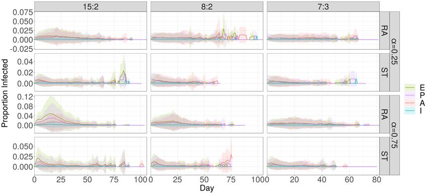
The pace of the outbreak is illustrated in Fig. 5, which shows the proportion of actively infected childcare centre attendees
(both children and educators) per day in each of the twelve scenarios. This figure shows that the 15:2 configuration tends to
produce a well-defined epidemic curve close to the start of the simulation, even with classroom closure protocols in place,
whereas 8:2 and 7:3 produce a more sporadic series of infection events throughout the simulation time horizon. In the case
of high transmission, the maximum mean level of exposure (E) is 2.54% in the 15:2 RA configuration 19 days into the
the simulation, on average, with peak 1.72% presymptomatic (P) and 1.2% asymptomatic (A) attendees at days 20 and 26
respectively. Meanwhile, peak mean exposure in scenario 7:3 ST comes on day 6, with 0.38% attendees exposed to the disease,
with presymptomatic cases never exceeding that of the start of the simulation.
4/26Figure 4. Diagram showing the proportion of trials without secondary spread (blue line, right x-axis), and the time taken to
produce the first secondary infection (bar chart), both sorted by scenario.
Figure 5. Time series of the proportions of exposed (E), presymptomatic (P), asymptomatic (A) and infected (I) individuals in
the simulation for each scenario. The ensemble means are represented by solid lines, while the respected shaded ribbons show
one standard deviation of the results.
Alternately, Table 2 summarizes the information from the figures, showing the days until the 30-day peak of each proportion
of active infections in the centre. Here we can see that active infections both peak far earlier with the ST allocation than
with the RA allocation for both high (α = 0.75) and low (α = 0.25) transmission rates, and have either equal or smaller
peaks than all maximum proportions corresponding to the RA allocation independent of student-educator ratio. There is no
obvious relationship between peak days for infected (I) and asymptomatic (A) individuals. In all cases (save status A in the
low transmission scenario and statuses P, E and I in the high transmission scenario, all with ST allocation), peak proportions
decreased consistently with the number of students per classroom. In sum, having fewer students per classroom and grouping
siblings together almost always results significantly lower peaks number of active infected and infectious cases in the school.
Peaks may also occur sooner in the ST allocation. This may reflect household members spending more time together than
under the RA allocation, resulting in a more rapid start to the outbreak even if the number of peak cases is more restricted under
the ST allocation.
5/26Peak Time Maximum
αC Status Allocation 15:2 8:2 7:3 15:2 8:2 7:3
RA 18 19 21 309 153 90
P
ST 4 0 0 128 98 82
RA 15 21 20 504 184 112
E
ST 3 3 3 211 139 96
0.75
RA 19 23 19 50 32 15
I
ST 4 3 8 17 20 15
RA 22 20 22 153 127 100
A
ST 5 6 8 55 63 50
αC Status Allocation 15:2 8:2 7:3 15:2 8:2 7:3
RA 18 0 0 93 83 72
P
ST 0 0 0 63 83 66
RA 21 3 9 110 70 46
E
ST 4 2 5 75 69 48
0.25
RA 21 28 2 20 15 14
I
ST 3 4 2 11 12 11
RA 21 11 29 87 60 60
A
ST 5 8 8 41 60 41
Table 2. Times at which the mean proportions of presymptomatic (P), exposed (E), symptomatically infected (I) and
asymptomatically infected (A) school attendees peak during the first 30 days of simulation with secondary spread with respect
to each of the scenarios tested, and the corresponding peak number of cases.
3.2 Outbreak size and duration
Each individual simulation ended when all classes were at full capacity and there were no active infections in the population;
aside from community infection, this marked the momentary stop of disease spread. From this, we get a description of the
duration of the first outbreak (there could well be a second outbreak sparked by some community infection among individuals
who remain susceptible at the end of the first outbreak). Box plots in Fig. 6 show that the 15:2 ratio in both RA and ST
allocations gives a much higher median outbreak duration than all other scenarios (for both low and high transmission cases).
Another general observation is that classroom allocation (RA vs. ST) doesn’t change the distribution of outbreak duration for
student-educator ratios 8:2 and 7:3 as drastically as it does for 15:2, whereas ST allocation results in a slightly higher median
duration but significantly lower maximum duration (54 vs. 85 for RA without outliers) in the high transmission case. This
is mirrored in the low transmission case as well. A possible explanation lies in the number of students per classroom. The
child-child contact rate (shown in Eqn. 3) is far higher than any other contact rate, implying that the classroom is the site
of greatest infection spread (demonstrated in Fig. 9). ST allocation differs from RA allocation in its containment of disease
transfer from the classroom to a comparatively limited number of households. This effect (the difference between ST and RA)
is amplified with the addition of each new student to the classroom, so that while the difference between 7:3 and 8:2 may be
small (only 1 student added), the effect becomes far exaggerated when the student number is effectively doubled (15 students
vs. 7 or 8).
The evolution of the numbers of susceptible (S) and recovered/removed (R) school attendees provides additional information
on the course of the outbreak, since they represent the terminal states of the disease progression experienced by every individual.
We recall that a classroom is closed as soon as one symptomatically infected case is identified, upon which every student and
teacher allocated to that room is sent home to begin the standard 14-day isolation period; asymptomatic students and teachers
return at the end of this period while symptomatic students remain at home and symptomatic teachers are replaced by substitutes.
As such, Fig. 7 shows the proportion of susceptible and recovered current school attendees. As with all results so far, the 15:2
RA scenario most efficiently facilitates disease spread through the childcare centre in both high and low transmission cases,
with the proportion of recovered (that is, previously ill) attendees (R) overtaking the number of never-infected attendees (status
S) on day 35 in the case of high transmission (α = 0.75). This intersection for all RA scenarios in the high transmission case,
and for all ratios but 7:3 in the low transmission case. Also, the point of intersection occurs further away from the outbreak
with less children in the classroom, again signifying faster disease spread facilitated by child-child interactions in the classroom
should the rate of transmission ever increase. Except for 15:2 in the high transmission case, there are no intersections of this
nature for ST scenarios (though the mean S and R proportions move toward intersection near the end of the simulation in all
high transmission scenarios). Performance between 8:2 and 7:3 with ST allocation is similar for both transmission rates, though
all scenarios show smaller variation over trials featuring lower infection transmission. As shown in Fig. 6, scenario 15:2 RA
6/26Figure 6. Box plots depicting the quartiles and outliers of simulation duration for each scenario. Taken together with the
stopping criteria of the simulations and measures of aggregate, these describe the duration of the outbreak. Red dots represent
the arithmetic mean of the data.
Figure 7. Time series detailing the trends in the mean proportions of current school attendees in each stage of disease
progression. Shaded ribbons around each curve show one standard deviation of the averaged time series. Only trials showing
secondary spread were included in the ensemble means shown.
gave the longest average simulation time in the high transmission scenario; this is also reflected in Fig. 5, where disease spread
halted (that is, the simulation satisfied the stopping criteria) only after > 105 days.
The relative importance of classroom interaction can be demonstrated by measuring the cumulative number of infections
occurring in specific locations over time. As can be seen in Fig. 8, these patterns vary depending on the transmissibility of the
infection. When the transmission rate is high (α = 0.75), infections in the classroom almost always exceed the total number
of infections in any other location. Especially for the 15:2 student-teacher ratio, the number of infections taking place in the
classroom is far higher with RA allocation than it is with ST allocation. Additionally, not only is the total number of infections
lower for the 8:2 and 7:3 student-teacher ratios with both classroom allocations, but so is the gap between classroom infections
and infections in the household. Transmission in common areas is low among all scenarios (as can be expected). For the
case of a low transmission rate (α = 0.25), infection is generally lower across all scenarios, and household infections outstrip
classroom infections for all scenarios except 15:2 RA.
Figure 9 shows the number of infections through the entire duration of the simulation in each location in all scenarios,
as well as the total number of infections in each scenario (the ‘outbreak size’). As expected, many more infections occur in
the high transmission scenario (α = 0.75), and the error bars of the plot show greater standard deviation of the results than
in the low transmission (α = 0.25) scenario. For each location in the model, the number of infections produces decreases
with the number of children interacting in the classroom; 15:2 is universally the worst allocation across all possible scenarios.
However, the difference between the numbers of produces infections in different scenarios decreases as the transmissibility of
the disease drops (so to speak, the gap been between the 15:2, RA and 15:2, ST scenarios decreases as α decreases, and so with
7/26Figure 8. Time series showing the cumulative number of infections occurring in each area of the school with respect to the
number of days open. Solid lines represent the ensemble mean, and shaded ribbons represent one standard deviation.
Figure 9. Bar chart showing the mean number of infections occurring among all school attendees in each location over time
for each scenario. The height of each bar gives the ensemble mean and its standard deviation is represented by error bars.
8/26Figure 10. Bar chart showing the number of days for which some number of rooms in the school were closed due to disease
outbreak. Scenarios are represented by different colours; the height of each bar gives the relevant ensemble mean with its
standard deviation represented by error bars.
other student-teacher ratios). When the transmission rate is high, the relatively larger variety (by household) and prevalence of
child-child interactions has a multiplicative effect on the number of effective transmissions in the class. Lower transmissibility
thereby decreases the efficiency of classroom infection relative to the potential for spread within households, which is seen by
the dominance of the household infection curve in Fig. 9.
3.3 Classroom closures and lost time
As noted before, when a symptomatic case (I) appears in the classroom, the classroom is shut down and all children and
teachers assigned to that room are sent home while the room remains closed. After 14 days, a closed classroom is reopened,
upon which recovered and remaining asymptomatic children and teachers will be allowed back. Since it’s possible for a student
or teacher to be infected during the closure period, not all attendees necessarily return to class upon reopening; sick teachers are
replaced with substitutes. As such, these class closures results in otherwise healthy students missing potentially many school
days. The numbers of student-days forfeited due to classroom closure are given in Fig. 11, according to scenario. (The number
of student-days forfeited is the number of days of closure times the number of students who would otherwise have been able to
continue attending.) In all scenarios, the 15:2 student-teacher ratio is quantitatively the worst strategy examined (by almost an
order of magnitude), resulting in the highest possible number of student days forfeited. Allocation scheme RA shows worse
performance than allocation ST in all scenarios, giving higher upper quartiles, maxima and outlying values. Both the low
(α = 0.25) and high (α = 0.75) transmissibility scenarios favour the 7:3 student-teacher ratio and ST allocation, with a lower
number of student days forfeited. The poor performance of 15:2 ratio occurs because it suffers from a multiplicative effect:
larger class sizes are more likely to be the origin of outbreak, and when the outbreak starts, more children are affected when the
classroom is shut down.
Naturally, a high rate of infection will result in multiple room closures; one way to see this is to look at the number and
duration of room closures, both shown in Fig. 10. In all scenarios, schools spent (on average) more days with one closed
classroom than any other number (0, 3-5). The only scenario for which all classrooms were closed for any significant stretch of
time was 15:2, RA in the case of low transmission rate. We can also observe a difference in RA and ST allocations for the 7:3
ratio; with both high and low transmission rate (α = 0.25 and α = 0.75 respectively), RA allocation results in a higher number
of class closures. The highest number of class closures seen for the 7:3, ST scenario was 2, whereas random assignment can
results in 4 or even closure of the entire school (due to the overlap of classroom closures, it’s not a significantly long period).
3.4 Sensitivity Analysis
We conducted a sensitivity analysis on β H , β C , λ and Rinit (see Methods for details). We found that rates of household and
classroom interaction and infection (β H and β C ) and the number of individuals initially recovered (Rinit ) greatly impact disease
spread in the model. However, variation in these parameters did not change the relative performances of the twelve scenarios
evaluated. The greatest influence on outcomes remain the scheme of allocation of students to classrooms (RA or ST), the
number of students per class (15, 8 or 7), and whether the transmission rate in the classrooms is low or high (αC ). Other
factors important to the spread of disease are classroom closure upon identification of a symptomatic case and the interaction
patterns of asymptomatic infected individuals in the household upon classroom closure (i.e. whether they continue to interact in
close contact, as would be necessary for younger children, or whether children are old enough to effectively self-isolate). Our
9/26Figure 11. Box plots showing the number of student days forfeited over the course of the simulation due to class closure upon
the detection of an outbreak. Red text boxes show the mean and standard deviation of closure.
baseline assumption was to assume asymptomatic infected individuals who are sent home due to closure of a classroom are
able to self-isolate. This assumption is conservative, since inability to self-isolate under these circumstances would result in
higher projected outbreak sizes.
4 Discussion
The present study developed and evaluated an agent-based model of COVID-19 transmission in a childcare setting for the
purposes of informing reopening policies. While the model was initialized for childcare, our findings are relevant for discussions
of school reopening, as well. Indeed, the model was configured to mimic COVID-19 transmission in a local school setting,
as many childcare centers operate across several classrooms within schools. These services are an essential bridge for many
parents who are unable to drop-off or pick-up children around school hours due to work. Our findings suggest that variability
in class size (i.e., number of children in a class) and class composition (i.e., sibling groupings versus random assignment)
influence the nature of COVID-19 transmission within the childcare context. Specifically, a 7:3 child-to-educator ratio that
utilized sibling groupings yielded the lowest rates of transmission, while a 15:2 ratio consistently performed far worse. Findings
from our simulations are sobering, as educators in the province are presently lobbying for a 15 student cap on classrooms. The
present study suggests that classes of this size pose a tangible risk for COVID-19 outbreaks, and that lower ratios would better
offset infection and school closures. While school reopening guidelines6 , public health agencies22 , and public petitions23 have
called for smaller class sizes, governments appear to be following some recommendations in reopening plans while ignoring
others.
Policies related to childcare and traditional school reopening have not been well integrated24 . In Ontario, childcare
classrooms were capped at a maximum of 10 occupants, overall (hence the 8:2 and 7:3 ratios in the present study)7 . Conversely,
procedures for traditional “school” classrooms have been given the go-ahead for 15 children (hence the 15:2 ratio). While
allowable class sizes will differ somewhat as a function of child age and jurisdiction, it seems likely that early childhood
and elementary school classes may actually surpass these numbers in Ontario. Our findings demonstrate that the 15:2 ratio
represents a significantly higher risk, not only for COVID-19 spread, but for school closures. In one scenario (15:2 random
assignment), the modeled outbreak lasted for 105 days. Given that childcare and schools are often operating within the same
physical location, this policy discrepancy is questionable. Based on our simulations, a lower ratio (7:3) is indicated. Moreover,
it appears that this configuration could be enhanced through the utilization of sibling groupings.
Our modelling approach was informative in terms of identifying the location of COVID-19 transmission. There has been
conflicting evidence on classroom based transmission of COVID-1925, 26 . The present study suggests that classrooms and
households yield much higher rates of infection than common areas. Thus, initiatives to reduce inter-classroom contact in
common areas (such as staggering start times, utilizing multiple entrances, and sanitizing surfaces in building foyers) may only
produce a modest benefit for reducing spread. Conversely, our simulations demonstrated a marked benefit associated with a
lower child-to-teacher ratios in classrooms. Notably, these benefits were observed in both high transmission settings (e.g., at
the start of the pandemic, before social distancing), and low transmission settings (e.g., where masking, hygiene, and social
distancing has been put in place, as will be the case in reopened childcare and school). Other investigators have proposed
intermittent occupancy and enhanced ventilation as potential measures for reducing classroom (indoor) transmission amongst
children27 .
10/26An examination of student days missed due to outbreaks (or school/classroom closure) further elucidates the favorability
of smaller class size and sibling grouping as a preventative measure. In this analysis, the worst configuration was the 15:2
random assignment ratio. Again, this was observed in both high transmission and low transmission environments. In the most
unfavorable scenario (15:2, random assignment), there were cumulatively 214 and 145 student days forfeited in high versus low
transmission settings, respectively. Conversely, in the best scenario (7:3, siblings together), there were only 13 and 16 student
days forfeited. Thus, our simulations suggest that the lower ratios and sibling groupings offer a safeguard against potential
breakdowns in infection control. Indeed, studies have suggested that school closures provide a modest benefit for preventing
COVID-19 spread, and may actually have unintended consequences by disrupting the labor force of healthcare workers28, 29 .
As such, a proactive and preventative approach would be better than a reactive strategy.
Several policy and procedural recommendations have emerged from this modeling exercise. First, it is recommended that
childcare and school settings, alike, consider lowering child-to-teacher ratios. Commensurate with the present findings, a 7:3
ratio (10 individuals per class including both children and adults) outperforms a 15:2 ratio on key metrics. Second, there also
appears to be benefit associated with sibling groupings. Thus, a siblings together configuration should be considered. Third, the
majority of transmission occurred in the classroom. As such, it is important for reopening plans to consider social distancing
and hygiene procedures within classrooms - a recommendation that may only be feasible with fewer children in the classroom.
It is unlikely that classrooms with 15 or more children will afford youngsters with the necessary space to socially distance.
Finally, the present study has a number of limitations that should be considered. While it is becoming increasingly clear that
COVID-19 risk varies as a function of social determinants of health (e.g., socioeconomic status, race, ethnicity, immigration
status, neighborhood risk), along with opportunities for social distancing30 , the present study did not take these considerations
into account. Future simulation studies might consider how these social determinants intersect with childcare and school
configurations. Additionally, this study was primarily concerned with COVID-19 infection and student days lost. That being
said, there are many important outcomes to consider in relation to children’s developmental health in the pandemic. Additional
longitudinal studies considering children’s learning and mental health outcomes in relation to new childcare and school
configurations are strongly indicated31 .
References
1. Cluver, L. et al. Parenting in a time of covid-19. The Lancet (2020).
2. Prime, H., Wade, M. & Browne, D. T. Risk and resilience in family well-being during the covid-19 pandemic. Am. Psychol.
(2020).
3. Stein-Zamir, C. et al. A large covid-19 outbreak in a high school 10 days after schools’ reopening, israel, may 2020.
Eurosurveillance 25, 2001352 (2020).
4. Melnick, H. et al. Reopening schools in the context of covid-19: Health and safety guidelines from other countries. Learn.
Policy Inst. (2020).
5. Christakis, D. A. School reopening—the pandemic issue that is not getting its due. JAMA pediatrics (2020).
6. SickKids. Covid-19: Guidance for school reopening. http://www.sickkids.ca/pdfs/about-sickkids/81407-covid19-
recommendations-for-school-reopening-sickkids.pdf (2020; accessed August 7, 2020).
7. of Ontario, G. Covid-19: reopening child care centres. http://www.edu.gov.on.ca/childcare/child-care-re-opening-
operational-guidance.pdf (2020; accessed August 7, 2020).
8. (Pan-InfORM, P. I. O. R. M. T. et al. Modelling an influenza pandemic: A guide for the perplexed. Cmaj 181, 171–173
(2009).
9. Bauch, C. T., Lloyd-Smith, J. O., Coffee, M. P. & Galvani, A. P. Dynamically modeling sars and other newly emerging
respiratory illnesses: past, present, and future. Epidemiology 791–801 (2005).
10. Park, S. W. et al. Reconciling early-outbreak estimates of the basic reproductive number and its uncertainty: framework
and applications to the novel coronavirus (sars-cov-2) outbreak. MedRxiv (2020).
11. Fraser, C., Riley, S., Anderson, R. M. & Ferguson, N. M. Factors that make an infectious disease outbreak controllable.
Proc. Natl. Acad. Sci. 101, 6146–6151 (2004).
12. Lee, B. Y. et al. Simulating school closure strategies to mitigate an influenza epidemic. J. public health management
practice: JPHMP 16, 252 (2010).
13. Ferguson, N. M. et al. Strategies for mitigating an influenza pandemic. Nature 442, 448–452 (2006).
14. Chitnis, N., Hyman, J. M. & Cushing, J. M. Determining important parameters in the spread of malaria through the
sensitivity analysis of a mathematical model. Bull. mathematical biology 70, 1272 (2008).
11/2615. Kumar, S., Grefenstette, J. J., Galloway, D., Albert, S. M. & Burke, D. S. Policies to reduce influenza in the workplace:
impact assessments using an agent-based model. Am. journal public health 103, 1406–1411 (2013).
16. Kretzschmar, M., van Duynhoven, Y. T. & Severijnen, A. J. Modeling prevention strategies for gonorrhea and chlamydia
using stochastic network simulations. Am. J. Epidemiol. 144, 306–317 (1996).
17. Wells, C. R., Klein, E. Y. & Bauch, C. T. Policy resistance undermines superspreader vaccination strategies for influenza.
PLoS Comput. Biol 9, e1002945 (2013).
18. Anderson, R. M., Anderson, B. & May, R. M. Infectious diseases of humans: dynamics and control (Oxford university
press, 1992).
19. Kucharski, A. J. et al. Effectiveness of isolation, testing, contact tracing and physical distancing on reducing transmission
of sars-cov-2 in different settings. medRxiv (2020).
20. Park, S. W., Cornforth, D. M., Dushoff, J. & Weitz, J. S. The time scale of asymptomatic transmission affects estimates of
epidemic potential in the covid-19 outbreak. medRxiv (2020).
21. Hellewell, J. et al. Feasibility of controlling covid-19 outbreaks by isolation of cases and contacts. The Lancet Glob. Heal.
(2020).
22. News, C. Toronto public health urges city’s largest school board to keep class sizes down.
https://www.cbc.ca/news/canada/toronto/toronto-public-health-school-guidance-1.5677739 (2020; accessed August 7,
2020).
23. Star, T. Thousands sign petition asking ontario to reduce class sizes for elementary school students
this fall. https://www.thestar.com/news/gta/2020/08/03/thousands-sign-petition-asking-ontario-to-reduce-class-sizes-for-
elementary-school-students-this-fall.html.
24. Dibner, K. A., Schweingruber, H. A. & Christakis, D. A. Reopening k-12 schools during the covid-19 pandemic: A report
from the national academies of sciences, engineering, and medicine. JAMA .
25. Heavey, L., Casey, G., Kelly, C., Kelly, D. & McDarby, G. No evidence of secondary transmission of covid-19 from
children attending school in ireland, 2020. Eurosurveillance 25, 2000903 (2020).
26. Shao, S. et al. Assessment of airborne transmission potential of covid-19 by asymptomatic individuals under different
practical settings. arXiv preprint arXiv:2007.03645 (2020).
27. Melikov, A., Ai, Z. & Markov, D. Intermittent occupancy combined with ventilation: An efficient strategy for the reduction
of airborne transmission indoors. Sci. The Total. Environ. 140908 (2020).
28. Bayham, J. & Fenichel, E. P. Impact of school closures for covid-19 on the us health-care workforce and net mortality: a
modelling study. The Lancet Public Heal. (2020).
29. Viner, R. M. et al. School closure and management practices during coronavirus outbreaks including covid-19: a rapid
systematic review. The Lancet Child & Adolesc. Heal. (2020).
30. Smith, J. A., de Dieu Basabose, J., Browne, D. T., Psych, C. & Stephenson, M. Family medicine with refugee newcomers
during the covid-19 crisis. .
31. Wade, M., Prime, H. & Browne, D. T. Why we need longitudinal mental health research with children and youth during
(and after) the covid-19 pandemic. Psychiatry Res. (2020).
32. Canada, S. Statistics canada 2016 census. https://www12.statcan.gc.ca/census-recensement/2016/dp-
pd/prof/details/page.cfm (accessed June 9, 2020).
33. Prem, K., Cook, A. R. & Jit, M. Projecting social contact matrices in 152 countries using contact surveys and demographic
data. PLoS computational biology 13, e1005697 (2017).
34. Koh, W. C. et al. What do we know about sars-cov-2 transmission? a systematic review and meta-analysis of the secondary
attack rate, serial interval, and asymptomatic infection. medRxiv (2020).
35. Public Health Ontario. Ontario covid-19 data tool. https://www.publichealthontario.ca/en/data-and-analysis/infectious-
disease/covid-19-data-surveillance/covid-19-data-tool (accessed June 10, 2020).
36. Lachmann, A. Correcting under-reported covid-19 case numbers. medRxiv (2020).
37. Nishiura, H., Linton, N. M. & Akhmetzhanov, A. R. Serial interval of novel coronavirus (2019-ncov) infections. medRxiv
(2020).
38. Tindale, L. et al. Transmission interval estimates suggest pre-symptomatic spread of COVID-19. medRxiv (2020).
12/265 Methods
5.1 Population Structure
There are N households in the population, and a single educational institution (either a childcare centre or a school, dependent
on scenarios to be introduced later) with M rooms and a maximum capacity dependent on the scenario being tested. Effective
contacts between individuals occur within each household, as well as rooms and common areas (entrances, bathrooms, hallways,
etc.) of the institution. All groups of individuals (households and rooms) in the model are assumed to be well-mixed.
Each individual (agent) in the model is assigned an age, household, room in the childcare facility and an epidemiological
status. Age is categorical, so that every individual is either considered a child (C) or an adult (A). Epidemiological status
is divided into stages in the progression of the disease; agents can either be susceptible (S), exposed to the disease (E),
presymptomatic (an initial asymptomatic infections period P), symptomatically infected (I), asymptomatically infected (A) or
removed/recovered (R), as show in Fig. 2.
In the model, some children in the population are enrolled as students in the institution and assigned a classroom based on
assumed scenarios of classroom occupancy while some adults are assigned teacher/caretaker roles in these classroom (again
dependent on the occupancy scenario being tested). Allocations are made such that there is only one teacher per household and
that children do not attend the same institution as a teacher in the household (if there is one), and vice versa.
5.2 Interaction and Disease Progression
The basic unit of time of the model is a single day, over which each attendee (of the institution) spends time at both home and at
the institution. The first interactions of each day are established within each household Hn , where all members of the household
interact with each other. An asymptomatically infectious individual of age i will transmit the disease to a susceptible housemate
with the age j with probability βi,Hj , while symptomatically infectious members will self-isolate (not interact with housemates)
for a period of 14 days.
The second set of interpersonal interactions occur within the institution. Individuals (both students and teachers) in each
room Rn interact with each other, where an infectious individual of age i transmits the disease to some susceptible individual of
age j with probability βi,Cj . To signify common areas within the building (such as hallways, bathrooms and entrances), each
individual will then interact with every other individual in the institution. There, an infectious individual of age j will infect a
susceptible individual of age i with probability βi,Oj .
To simulate community transmission (for example, public transport, coffee shops and other sources of infection not explicitly
modelled here), each susceptible attendee is infected with probability λS . Susceptible individuals not attending the institution in
some capacity are infected at rate λN , where λN > λS to compensate for those consistent effective interactions outside of the
institution that are neglected by the model (such as workplace interactions among essential workers and members of the public).
Figure 2 shows the progression of the illness experienced by each individual in the model. In each day, susceptible (S)
individuals exposed to the disease via community spread or interaction with infectious individuals (those with disease statuses P,
A and I) become exposed (E), while previously exposed agents become presymptomatic (P) with probability δ . Presymptomatic
agents develop an infection in each day with probability δ , where they can either become symptomatically infected (I) with
probability η or asymptomatically infected (A) with probability 1 − η.
The capacity of sole educational institution in the model is divided evenly between 5 rooms, with class size and teacher-
student ratio governed by one of three scenarios: seven students and three teachers per room (7 : 3), eight students and two
teachers per room (8 : 2), and fifteen students and two teachers per room (15 : 2). Classroom allocations for children can be
either randomised or grouped by household (siblings are put in the same class).
Symptomatically infected agents (I) are removed from the simulation after 1 day (status R) with probability γI , upon which
they self-isolate for 14 days, and therefore no longer pose a risk to susceptible individuals. Asymptomatically infected agents
(A) remain infectious but are presumed able to maintain regular effective contact with other individuals in the population due to
their lack of noticeable symptoms; they recover during this period (status R) with probability γA . Disease statuses are updated
at the end of each day, after which the cycles of interaction and infection reoccur the next day.
The actions of symptomatic (status I) agents depend on age and role. Individuals that become symptomatic maintain a
regular schedule for 1 day following initial infection (including effective interaction within the institution, if attending), after
which they serve a mandatory 14-day isolation period at home during which they interaction with no one (including other
members of their household). On the second day after the individual’s development of symptoms, their infection is considered a
disease outbreak centred in their assigned room, triggering the closure of that room for 14 days. All individuals assigned to that
room are sent home, where they self-isolate for 14 days due to presumed exposure to the disease. Symptomatically infected
children are not replaced, and simply return to their assigned classroom upon recovery. At the time of classroom reopening, any
symptomatic teacher is replaced by a substitute for the duration of their recovery, upon which they reprise their previous role in
the institution; the selection of a substitute is made under previous constraints on teacher selection (one teacher per household.
with no one chosen from households hosting any children currently enrolled in the institution).
13/265.3 Parameterization
The parameter values given in Tab. 4. The sizes of households in the simulation was determined from 2016 Statistics Canada
census data on the distribution of family sizes32 as seen in Tab. 3.
Probability # Adults # Children Probability # Adults # Children
0.169 1 1 0.284 2 1
0.079 1 2 0.307 2 2
0.019 1 3 0.086 2 3
0.007 1 4 0.033 2 4
0.003 1 5 0.012 2 5
(a) Households not hosting teachers.
Probability # Adults
0.282 1
0.345 2
0.152 3
0.138 4
0.055 5
0.021 6
0.009 7
(b) Households hosting teachers.
Table 3. Tables showing distributions of the sizes and adult-child ratios of the two types of households used in this study.
The proportion of single and two parent homes not hosting teachers is shown in Tab. 3a. We note that Statistics Canada data
only report family sizes of 1, 2 or 3 children: the relative proportions for 3+ children were obtained by assuming that 65% of
families of 3+ children had 3 children, 25% had 4 children, 10% had 5 children, and none had more than 5 children. Each
teacher was assumed to be a member of a household that did not have children attending the school. Again using census data,
we assumed that 36% of teachers live in homes with no children, the sizes of which follow the distribution given in Tab. 3b.
Others live with ≥ 1 children in households following the size and composition distribution shown in Tab. 3a.
The age-specific transmission rates in households are given by the matrix:
H H H H
β1,1 β1,2 H c1,1 c1,2
H H ≡β cH H , (1)
β2,1 β2,2 2,1 c2,2
where cH 33
i, j gives the number of contacts per day reported between individuals of ages i and j estimated from data and the
baseline transmission rate β H is calibrated. To estimate cH 33
i, j from the data in Ref. , we used the non-physical contacts of age
class 0-9 years and 25-44 years of age, with themselves and one another, in Canadian households. Based on a meta-analysis,
the secondary attack rate of COVID-19 appears to be approximately 15% on average in both Asian and Western households34 .
Hence, we calibrated β H such that a given susceptible person had a 15% chance of being infected by a single infected person in
their own household over the duration of their infection averaged across all scenarios tested (App. 5.5). As such, age specific
transmission is given by the matrix
H 0.5378 0.3916
β · . (2)
0.3632 0.3335
To determine λS we used case notification data from Ontario during lockdown, when schools, workplaces, and schools
were closed35 . During this period, Ontario reported approximately 200 cases per day. The Ontario population size is 14.6
million, so this corresponds to a daily infection probability of 1.37 × 10⁻⁵ per person. However, cases are under-ascertained by
a significant factor in many countries36 –we assumed an under-ascertainment factor of 8.45, meaning there are actually 8.45
times more cases than reported in Ontario, giving rise to λS = 1.16 × 10⁻⁴ per day; λN was set to 2 · λS .
The age-specific transmission rates in the school rooms is given by the matrix
C C C C
β1,1 β1,2 C c1,1 c1,2 C 1.2356 0.0588
C C ≡ β ≡ β , (3)
β2,1 β2,2 cC2,1 cC2,2 0.1176 0.0451
where cCi, j is the number of contacts per day reported between age i and j estimated from data33 . To estimate cCi, j from the data
in Ref.33 , we used the non-physical contacts of age class 0-9 years and 20-54 years of age, with themselves and one another, in
14/26Canadian schools. Epidemiological data on secondary attack rates in childcare settings are rare, since schools and schools were
closed early in the outbreak in most areas. We note that contacts in families are qualitatively similar in nature and duration
to contacts in schools with small group sizes, although we contacts are generally more dispersed among the larger groups in
rooms, than among the smaller groups in households. On the other hand, rooms may represent equally favourable conditions
for aerosol transmission, as opposed to close contact. Hence, we assumed that β C = αC β H , with a baseline value of αC = 0.75
based on more dispersed contacts expected in the larger room group, although we varied this assumption in sensitivity analysis.
To determine β O we assumed that β O = αO β C where αO
1 to account for the fact that students spend less time in
common areas than in their rooms. To estimate αO , we note that β O is the probability that a given infected person transmits
the infection to a given susceptible person. If students and staff have a probability p per hour of visiting a common area, then
their chance of meeting a given other student/staff in the same area in that area is p2 . We assumed that p = 0.05 and thus
αO = 0.0025. The age-specific contact matrix for βO was the same as that used for β C (Eqn. 3).
5.4 Model Initialisation
Upon population generation, each agent is initially susceptible (S). Individuals are assigned to households as described in the
Parameterisation section, and children are assigned to rooms either randomly or by household. We assume that parents in
households with more than one child will decide to enroll their children in the same institution for convenience with probability
ξ = 80%, so that each additional child in multi-child households will have probability 1 − ξ of not being assigned to the
institution being modelled.
Households hosting teachers are generated separately. As in the Parameterisation section, we assume that 36% of teachers
live in adult-only houses, while the other teachers live in houses with children, both household sizes following the distributions
outlined in Tab. 3. The number of teacher households is twice that required to fully supply the school due to the replacement
process for symptomatic teachers outlined in the Disease Progression section.
Initially, a proportion of all susceptible agents Rinit is marked as removed/recovered (R) to account for immunity caused by
previous infection moving through the population. A single randomly chosen primary case is made presymptomatic (P) to
introduce a source of infection to the model. All simulations are run until there are no more potentially infectious (E, P, I, A)
individuals left in the population and the institution is at full capacity.
All results were averaged over 2000 trials.
Parameter Meaning Baseline Value Source
η probability of symptomatic infection 0.6 (adults) TBD
0.4 (children) TBD
δ transition probability, E → P 0.5/day 37, 38
σ transition probability, P → I, A 0.5/day 37, 38
γI transition probability, I → R 1.0/day 37, 38
γA transition probability, A → R 0.25/day 37, 38
cH household contact matrix ... 33
ij
βH transmission probability in households 0.109 34 , calibrated
cCij room contact matrix ... 33
βC transmission probability in classrooms β C = αC β H , 34 , assumption
αC = 0.75
βiOj transmission probability in common areas β O = αO β C , 33, 34 , assumption
αO = 0.0025
λi infection rate due to other sources 1.16 × 10⁻⁴ /day 35 ,estimated
Rinit initial proportion with immunity 0.1 assumption
ξ probability of sibling attending same centre 0.8 assumption
o proportion of childless teachers 0.36 32 , assumption
household size distributions 32
Table 4. Parameter definitions, baseline values and literature sources.
5.5 Estimating β H
Agents in the simulation were divided into two classes: “children” (ages 0 − 9) and “adults” (ages 25 − 44). Available data
on contact rates33 was stratified into age categories of width 5 years starting at age 0 (0 − 5. 5 − 9, 10 − 14, etc.). The mean
15/26number of contacts per day cH i, j for each class we considered (shown in Eq. 2) was estimated by taking the mean of the contact
rates of all age classes fitting within our presumed age ranges for children and adults.
For β H calibration, we created populations by generating a sufficient number of households to fill the institution in each of
the three tested scenarios; 15 : 2, 8 : 2 and 7 : 3. In each household, a single randomly chosen individual was infected (each
member with equal probability) by assigning them a presymptomatic disease status P; all other members were marked as
susceptible (disease status S). In each day of the simulation, each member of each household was allowed to interact with the
infected member, becoming exposed to the disease with probability given in Eqn. 2. Upon exposure, they were assigned disease
status E. At the beginning of each subsequent day, presymptomatic individuals proceeded to infected statuses I and A, and
infected agents were allowed to recover as dictated by Fig. 2 and Tab. 4. This cycle of interaction and recovery within each
household was allowed to continue until all infected individuals were recovered from illness.
We did not allow exposed agents (status E) to progress to an infectious stage (I or A) since we were interested in finding
out how many infections within the household would result from a single infected household member, as opposed to added
secondary infections in later days. At the end of each trial, the specific probability of infection (πn ) in each household Hn was
calculated by dividing the number of exposed agents in the household (En ) by the size of the household |Hn | less 1 (accounting
for the member initially infected). Single occupant households (|Hn | = 1) were excluded from the calculation. The total
probability of infection π was then taken as the mean of all πn , so that
1 1 En
π= πn = ∑ |Hn | − 1 , (4)
D∑n D |H |≥2
n
where D represents the total number of multiple occupancy households in the simulation. This modified disease simulation
was run for 2000 trials each of different prospective values of β H ranging from 0 to 0.21. The means of all corresponding
final estimates of the infection rate were taken per value of β H , and the value corresponding to a infection rate of 15% was
interpolated, as shown in Fig. 12.
Figure 12. Plot showing the probability of infection stemming from single infection in the household with respect to the value
of the contact rate coefficient β H . The shaded region represents one standard deviation of ensemble values obtained for each
value of β H .
5.6 Sensitivity Analysis: varying α0 and BH
In Fig. 13, the mean number of student days missed decreases with the number of students per classroom for all values of
parameter combinations shown, reinforcing the idea that student-student classroom interaction is one of the main drivers of
model behaviour. Specifically, decreases are much more pronounced for RA allocation and ST allocation. Further, for each
value of α0 , increases in β H from low to high values brought the number of missed student from their respectively different
initial values to roughly the same maximum values for all values of α0 . For instance, in scenario α0 = 0.00125, 15:2 RA,
the number of forfeited days increases from 111.5 ± 202.1 to 261 ± 307.2, while higher α0 = 0.00375 brings an increase
from 116.4 ± 209.9 to 263.1 ± 303.9; indeed, α0 exerts much less influence over the number of forfeited days than does β H ,
suggesting that common area infection (though seeming important due to the number of students involved) is not largely
responsible for the number of student days forfeited. It should be noted that the standard deviations of these measurement
dwarf the mean itself, yet still the distribution of values can be seen as changing.
16/26You can also read