In-situ Image Analysis of Habitat Heterogeneity and Benthic Biodiversity in the Prince Gustav Channel, Eastern Antarctic Peninsula - Frontiers
←
→
Page content transcription
If your browser does not render page correctly, please read the page content below
ORIGINAL RESEARCH
                                                                                                                                           published: 28 January 2021
                                                                                                                                     doi: 10.3389/fmars.2021.614496

                                             In-situ Image Analysis of Habitat
                                             Heterogeneity and Benthic
                                             Biodiversity in the Prince Gustav
                                             Channel, Eastern Antarctic Peninsula
                                             Peter M. Almond 1*, Katrin Linse 2 , Simon Dreutter 3 , Susie M. Grant 2 , Huw J. Griffiths 2 ,
                                             Rowan J. Whittle 2 , Melanie Mackenzie 4 and William D. K. Reid 1*
                                             1
                                              School of Natural and Environmental Sciences, Newcastle University, Newcastle upon Tyne, United Kingdom, 2 British
                                             Antarctic Survey, Cambridge, United Kingdom, 3 Alfred Wegener Institute, Bremerhaven, Germany, 4 Museums Victoria,
                                             Melbourne, VIC, Australia

                          Edited by:
                      Wei-Jen Chen,          Habitat heterogeneity is important for maintaining high levels of benthic biodiversity. The
    National Taiwan University, Taiwan       Prince Gustav Channel, on the Eastern Antarctic Peninsula, is characterized by an array
                         Reviewed by:        of habitat types, ranging from flat, mud-dominated sheltered bays to steep and rocky
                             Karine Olu,
  Institut Français de Recherche pour        exposed slopes. The channel has undergone dramatic environmental changes in recent
                l’Exploitation de la Mer     decades, with the southern end of the channel permanently covered by the Prince Gustav
                    (IFREMER), France
                                             Ice Shelf until it completely collapsed in 1995. Until now the marine benthic fauna of the
                         Ann Vanreusel,
              Ghent University, Belgium      Prince Gustav Channel has remained unstudied. A shallow underwater camera system
                   *Correspondence:          and Agassiz trawl were deployed at different locations across the channel to collect
                      Peter M. Almond        information on habitat type and heterogeneity, benthic community composition and
          p.almond@newcastle.ac.uk
                     William D. K. Reid      macrofaunal biomass. The texture of the seafloor was found to have a significant influence
         william.reid@newcastle.ac.uk        on the benthos, with hard substrates supporting higher abundances and diversity.
                                             Suspension and filter feeding organisms, including porifera, crinoids, and anthozoans,
                  Specialty section:
        This article was submitted to
                                             were strongly associated with hard substrates, with the same being true for deposit
        Marine Evolutionary Biology,         feeders, such as holothurians, and soft sediments. Habitat heterogeneity was high across
 Biogeography and Species Diversity,
                                             the Prince Gustav Channel, particularly on a local scale, and this was significant in
              a section of the journal
         Frontiers in Marine Science         determining patterns of benthic composition and abundance. Other physical variables
         Received: 06 October 2020           including depth and seafloor gradient played significant, interactive roles in determining
         Accepted: 06 January 2021           composition potentially mediated through other processes. Sites that were once covered
         Published: 28 January 2021
                                             by the Prince Gustav Ice Shelf held distinct and unique communities, suggesting that the
                             Citation:
    Almond PM, Linse K, Dreutter S,
                                             legacy of the ice shelf collapse may still be reflected in the benthos. Biomass estimations
  Grant SM, Griffiths HJ, Whittle RJ,        suggest that critical thresholds of vulnerable marine ecosystem indicator taxa, as defined
 Mackenzie M and Reid WDK (2021)             by the Commission for the Conservation of Antarctic Marine Living Resources, have been
    In-situ Image Analysis of Habitat
          Heterogeneity and Benthic          met at multiple locations within the Prince Gustav Channel, which has implications for
    Biodiversity in the Prince Gustav        the future establishment of no take zones and marine protected areas within the region.
Channel, Eastern Antarctic Peninsula.
           Front. Mar. Sci. 8:614496.        Keywords: vulnerable marine ecosystem, habitat heterogeneity, benthic biodiversity, global climate change, ice
   doi: 10.3389/fmars.2021.614496            shelf, marine protect area, Antarctic

Frontiers in Marine Science | www.frontiersin.org                                  1                                         January 2021 | Volume 8 | Article 614496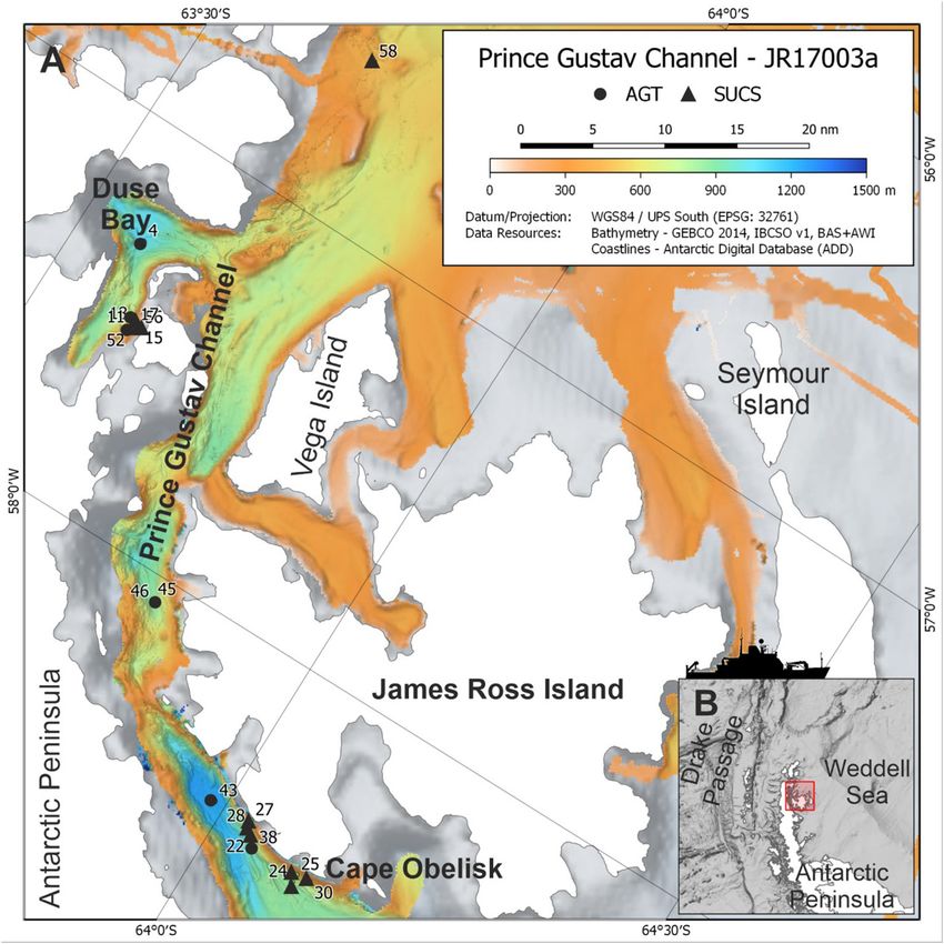
Almond et al.                                                                                  Habitat Heterogeneity and Benthic Biodiversity in the PGC

INTRODUCTION                                                               of fisheries and conservation of marine ecosystems throughout
                                                                           the Southern Ocean. Part of CCAMLR’s remit is the identification
The Antarctic continental shelf and slope is characterized by a            and protection of Vulnerable Marine Ecosystems (VMEs) to
highly diverse benthos that displays high levels of endemism               protect benthic habitats from the adverse impacts of bottom
and spatial variability (Convey et al., 2014). All main types of           fishing activities (CCAMLR, 2009a; Parker and Bowden, 2010).
macrobenthic communities, in particular suspension and mobile              To facilitate this, CCAMLR developed a classification of VME
or deposit feeders, can occur all around the Southern Ocean,               indicator organisms (CCAMLR, 2009b), taxa deemed potentially
which suggests that their distribution on a regional and local             vulnerable to the impacts of bottom fishing. Conservation
scale is likely unpredictable and assumed to be shaped by                  Measures dictate that when specific thresholds of VME taxa
complex biological and physical interactions (Gutt et al., 2013).          biomass are met, specifically 10 kg of biomass per 1200 m
Measuring species and biological diversity on the Antarctic shelf          longline, these areas will be defined as “VME Risk Area” and
is notoriously difficult as a result of high community patchiness          are then to be closed to fishing activities until management
and complex hierarchical scales of spatial variation (Thrush et al.,       decisions can be determined by the Commission (CCAMLR,
2006). Additionally, sampling gaps limit our understanding of the          2009a). Several previous studies based on the Antarctic shelf
processes at work (Griffiths, 2010). Current biodiversity estimates        and slope have provided data on VME biomass that have been
come either from regions which vary from small, well-sampled               useful for the notification of VME Risk Areas, as week as the
locations such as King George Island or the South Orkney Islands           development of protected areas within the region (Parker and
to areas like the Amundsen Sea, which spans a large area but               Bowden, 2010; Lockhart and Hocevar, 2018).
where no fauna had been collected prior to 2008 (Kaiser et al.,                The Prince Gustav Channel (PGC) is located at the north-
2009). The development of statistical and modeling methods                 eastern tip of the Antarctic Peninsula, defined by the Peninsula
using the to-date knowledge on all known or described Antarctic            itself to the west and James Ross Island to the east. The channel
species are also useful in the development of biodiversity                 extends to the Antarctic Sound and Andersson Island to the
estimates (Gutt et al., 2004). Constraining interactions between           north, including Eagle Island and the associated Duse Bay, and
physical and biological variables is vital for understanding drivers       reaches Cape Obelisk at the very south. The south region of the
of Antarctic biodiversity and enabling development of predictive           channel was covered by the Prince Gustav Ice Shelf, which was
ecological models (Convey et al., 2014). Physical datasets are             more than 15 nautical miles across and included Ross Bay and
available across larger scales than biological observations, with          part of James Ross Island (Cook and Vaughan, 2010). The ice shelf
broad-scale bathymetric, geomorphological, temperature, sea ice            began to collapse in the mid-19th century, and by 1995 the PGC
patterns, and more available from observations and satellite data          was completely open throughout its length during the austral
(Post et al., 2014). Thus, physical datasets provide an opportunity        summer (Cooper, 1997). By these same estimates, the ice shelf
to build predictive models of species distributions and diversity if       still permanently covered the sea at Cape Obelisk as recently as
significant relationships can be established. Such models can be           1989, making this a relatively newly uncovered area of seafloor.
significant for guiding Southern Ocean ecosystem management,               The southern part of the channel was included in a proposed
including the selection and monitoring of Marine Protected                 Weddell Sea MPA presented to CCAMLR in 2016 (Teschke
Areas (MPAs).                                                              et al., 2016). CCAMLR has not yet reached an agreement on
    Habitat heterogeneity and substrate characteristics have been          the proposal.
found to be important determinants of benthic community                        The goal of the present research was to investigate the benthic
composition in the South Orkney Islands, Ross Sea, and East                community of the PGC and how these relate to aspects of habitat
Antarctica (Cummings et al., 2006; Post et al., 2017; Brasier              complexity and heterogeneity. Specifically, the aims were to: (1)
et al., 2018), while in other regions the relationship between             describe the physical habitat characteristics and overall structure
the benthos and substrate is less consistent (Gutt et al., 2016).          of the benthos at sites across the PGC; (2) investigate how
These patterns vary between regions, and there is little if any            these communities vary across different regions and depths; (3)
clear evidence relationships between biodiversity and depth,               establish the physical variables that are associated with differences
latitude or environmental parameters that can be applied to                in community structure (4) investigate the abundance and
benthos across the whole Southern Ocean (Brandt et al., 2007).             distribution associated with VME taxa. This study represents the
In addition to developing broad-scale biodiversity models, it is           first assessment of the benthic community of the PGC. It provides
important to consider the significance of fine-scale variability and       an opportunity to assess the implications for conservation and
its impact on biological communities. The complex interplay of             management for this section of the Weddell Sea and establish
different biological and physical factors creates habitat patchiness       a baseline for assessing the impacts of future biological or
at a range of scales that significantly enhance biological diversity       environmental changes that occur in the region.
on the Antarctic shelf on both a local and regional scale (Gutt
and Piepenburg, 2003). The impacts of variations in physical
                                                                           MATERIALS AND METHODS
determiners are mediated by the biological characteristics and
life history traits of the local fauna, including mode of dispersal,       Data Collection
growth rate, and functional role (Gutt and Koltun, 1995).                  In 2018, the RSS James Clark Ross expedition JR17003a sampled
    The Commission for the Conservation of Antarctic Marine                four sites within the PGC and one site north of the PGC
Living Resources (CCAMLR) is responsible for the management                in the vicinity of Andersson Island between 63◦ 30′ S and

Frontiers in Marine Science | www.frontiersin.org                      2                                       January 2021 | Volume 8 | Article 614496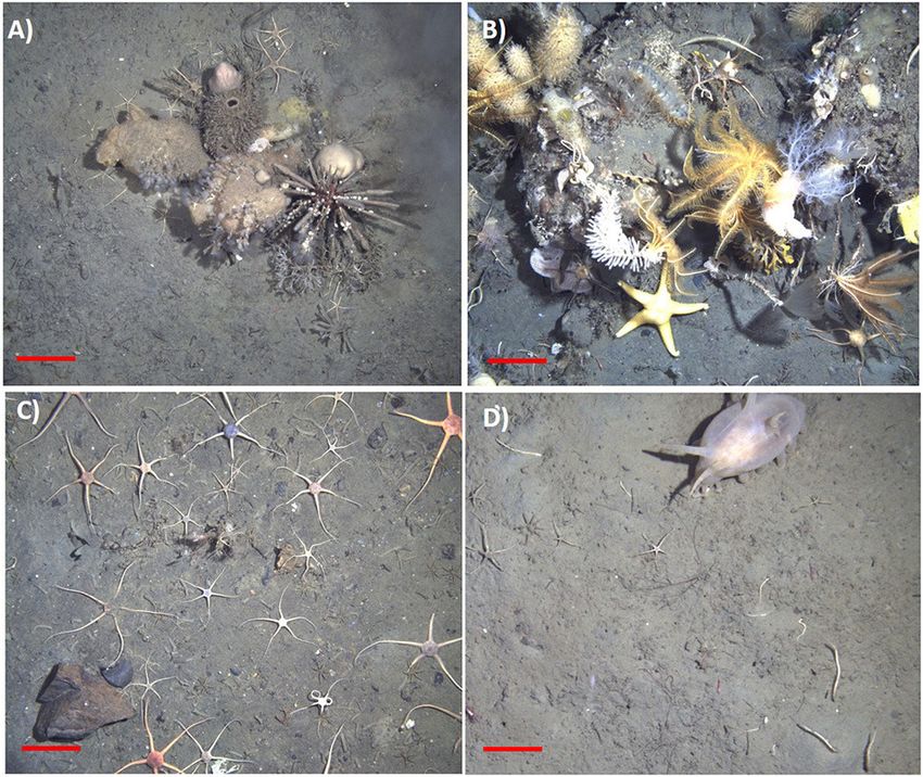
Almond et al.                                                                                           Habitat Heterogeneity and Benthic Biodiversity in the PGC

64◦ 8′ S (Figure 1; Table 1). Before deployment of the Shallow                    was deployed six times across three locations, all of which were
Underwater Camera System (SUCS) and Agassiz Trawl (AGT),                          also sampled using the SUCS (Table 1). The AGT had a mouth
multibeam bathymetry data were collected to ascertain seafloor                    width of 2 m and a mesh size of 1 cm. It was trawled at 1 knot for
topography, slope gradient, and suitability for deployment of                     2–10 min. These provided reference specimens to help identify
these sampling gears. The sampling covered depths between                         species in the SUCS images. Five trawls were identified to the
200 and 1200 m, although not all depths were sampled at                           lowest possible taxonomic level and sorted during the cruise
each location because of either ice cover or unsuitable seafloor                  while the final trawl was fixed in bulk in 99.8% absolute ethanol
topography (Table 1). The SUCS is a tethered drop-camera                          and sorted at a later date. The wet weight (biomass) of all different
system with an HD camera and live feed back to the ship. The                      taxa was assessed on board using calibrated scales. Topography
system allows the capture of high-resolution images (2448 ×                       and presence of pack-ice meant that not all locations where SUCS
2050 pixels) covering 0.51 m2 of seafloor. It was deployed 12                     sampling was undertaken had a corresponding AGT sample.
times across the five locations (Table 1). Each deployment was
at a unique depth within that location and consisted of three                     Image Analysis
transects of 10 photos. Each photo within a transect was taken                    All organisms in each SUCS image were identified to the lowest
10 m apart. At the end of each transect the SUCS was moved                        possible taxonomic level, or to morphospecies, dependent on
100 m to begin the next. The direction of the transects was                       resolution of the images and cross-checked where possible
determined by the wind direction and topography. In some cases,                   with taxa identified from the AGT trawls at the corresponding
not all the transects could be completed because of icebergs in                   location and depth. Some biological material was unidentifiable
close vicinity to the vessel or problems with the gear. The AGT                   to phyla but distinguishable as VME species, for example

 FIGURE 1 | Map of study area. (A) Station locations of SUCS and AGT deployments during JR17003a, including event deployment numbers. (B) Position of the
 Prince Gustav Channel on the Antarctic Peninsula in the Southern Ocean. Bathymetry data archived from Dreutter et al. (2020).

Frontiers in Marine Science | www.frontiersin.org                             3                                         January 2021 | Volume 8 | Article 614496
Almond et al.                                                                                                             Habitat Heterogeneity and Benthic Biodiversity in the PGC

TABLE 1 | Station details for SUCS and AGT deployments.

Region                                Station number SUCS/             Deptha      Latitudeb      Longitudeb           Transects/No. of          Trawl time in            Date
                                        AGT* Deployment                                                                 photos (SUCS)            minutes (AGT)

Duse Bay                                          11                    500 m      −63.6154        −57.4976                 3/30                        -              02/03/2018
                                                  15                    200 m      −63.6243        −57.4821                 3/30                        -              02/03/2018
                                                  17                    300 m       −63.619        −57.4848                 3/30                        -              02/03/2018
                                                  18                    400 m      −63.6154        −57.4869                 3/30                        -              02/03/2018
                                                   4*                  1000 m      −63.5755        −57.2954                   -                        10              01/03/2018
                                                  52*                   500 m      −63.6161        −57.5035                   -                         5              07/03/2018
                                                  56*                   200 m      −63.6253        −57.4863                   -                         2              07/03/2018
Prince Gustav Channel Mid
                                                  45                    850 m      −63.8044        −58.0632                 3/29                        -              06/03/2018
                                                  46*                   850 m      −63.8082        −58.0677                   -                         5              06/03/2018
Prince Gustav Channel–South
                                                  22                    800 m      −64.0412        −58.4526                 3/26                        -              03/03/2018
                                                  27                    200 m      −64.0333        −58.4185                 3/30                        -              04/03/2018
                                                  28                    500 m      −64.0363        −58.4328                 3/30                        -              04/03/2018
                                                  38*                   800 m      −64.0552        −58.4765                   -                         5              05/03/2018
                                                  43*                  1200 m      −63.9881        −58.4225                   -                         5              06/03/2018
Cape Obelisk
                                                  24                    800 m       −64.111        −58.4995                 3/30                        -              03/03/2018
                                                  25                    500 m      −64.1108        −58.4777                 3/30                        -              03/03/2018
                                                  30                    400 m       −64.128        −58.4750                 3/30                        -              04/03/2018
Andersson Island
                                                  58                    500 m      −63.6846        −56.5787                 3/30                        -              06/03/2018

*AGT; a General station depth, b Coordinates for start of first transect (SUCS) and net reaching the seafloor (AGT).

branched or budding fragments which were identifiable as                                         and converted into proportion of total catch to allow for
cnidarian or bryozoan species. These individuals were classed                                    comparison of proportional catch between gear type. As the
as “VME unidentifiable.” Length-weight relationships were                                        sample size was relatively low, no significant statistical analysis
used to estimate VME biomass present in the SUCS imagery,                                        was carried out on AGT data. The observable taxa in each image
derived from measurements of specimens collected from the                                        of the SUCS were counted and an ANOVA was used to test
South Orkney Islands (Brasier et al., 2018). SUCS images were                                    the difference among sample sites within the PGC. Diversity
used to investigate the relationships between habitat type and                                   measures (Simpson’s index and Shannon-Weiner index) were
community structure. The percentage cover of different substrate                                 calculated for each photo using the total number of individuals
types in each image was recorded. Substrate was classified as                                    and the total number of different taxa present in any given photo
either mud, sand, gravel, pebbles, cobbles, boulders (which                                      using the Vegan package for R (Oksanen et al., 2011). These
included dropstones) or bedrock, based on size classifications                                   measures were chosen as each can be used to infer different
from Sedimentary Petrology: An Introduction to the Origin of                                     information about the community, and both can be viewed
Sedimentary Rocks (Tucker, 1991). Substrate size classifications                                 as appropriate representations in marine systems (Washington,
were adjusted to align with the image size on screen using                                       1984). While Shannon-Weiner represents a combination of both
the known SUCS field of view (0.51 m2 ). Each image was                                          species richness and equitability in distribution among a sample,
assigned a texture, based on the dominating substrate type                                       Simpson’s is weighted toward more abundant species in a sample,
in each image, with mud and sand classified as “Soft” and                                        thereby giving an impression of species dominance within a
all others as “Hard.” Biogenic substrate was also determined                                     system. Estimated VME biomass over 1200 m2 (the area used
as percentage cover of each photo. Biogenic substrate refers                                     by CCAMLR to define a VME Risk Area) (CCAMLR, 2009a)
to any ecosystem engineering organisms that create a three-                                      was calculated using the known area of the SUCS field of view
dimensional structure that contributes to the given habitat. This                                (0.51 m2 ), where wet weight over 1200 m2 = (average weight ×
included organisms such as Porifera, tube forming polychaeta                                     1.961) × 1200.
and Ascidians, Cnidaria and Bryozoa.                                                                Beta-diversity and the degree to which benthic habitat
                                                                                                 characteristics were associated with the benthos were analyzed
Data Analysis                                                                                    using a combination of correspondence analysis (CA) and
Data analysis was performed in RStudio, version 1.3.1056. All                                    canonical correspondence analysis (CCA) using the Vegan
organisms observed in the SUCS images and AGT were totalled                                      package for R. The CA site scores from the ordination represent

Frontiers in Marine Science | www.frontiersin.org                                            4                                            January 2021 | Volume 8 | Article 614496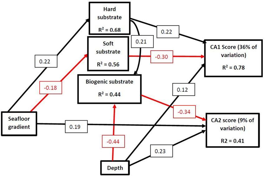
Almond et al. Habitat Heterogeneity and Benthic Biodiversity in the PGC
the similarity between sites. The result is that two sites with
similar CA scores have a very similar composition of benthic
fauna whereas those with widely different CA scores contain a
very different collection of benthic fauna. Any major trend in the
first axis represents the degree to which the benthic community
turns over along an environmental gradient. The CA scores are
used as a measure of beta-diversity. The beta-diversity estimates
will be based on the images from the SUCS so will represent the
epibenthic fauna that are visible. A structural equational model
(SEM) was used to determine the direct and indirect effects of
physical variables on beta-diversity. SEMs are a regression-based
approach to evaluating causal links between multiple variables
in a multivariate system (Lefcheck, 2016). This approach allows
variables to function as both predictors and responses within a
single model allowing the identification of indirect effects and
the testing of specific hypotheses on the interactions between
these variables. The SEM was constructed using the R-package
piecewiseSEM (Lefcheck, 2016), which allows for the inclusion of
non-normally distributed response variables and random effects
that account for non-independence in the data. CA1 and CA2
axis scores were used as proxies to represent beta-diversity. The
SEM had two indirect pathways, which flow from depth and slope
angle to substrate cover and on to CA1 and CA2 scores. Depth
and slope angle also have direct pathways to CA1 and CA2, which
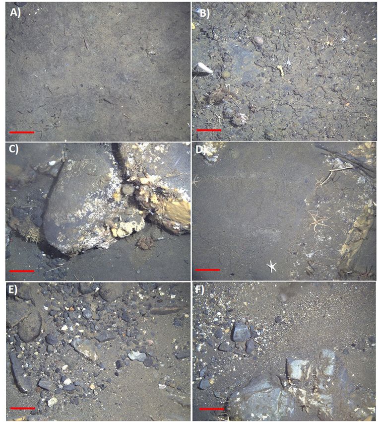
FIGURE 2 | Examples of in-situ SUCS images showing different substrate
allow evaluation of whether any depth or slope related change
classifications. (A) Mud dominated, (B) gravel and small pebbles above
are due to changes in the indirect pathways or due to a different exposed bedrock, (C) boulders/dropstones, (D) sandy bottom with some
unmeasured variable. A second SEM was used to investigate the exposed boulders, (E) gravel and small pebbles, and (F) mixture of sand,
indirect and direct effects of slope, depth, and substrate cover gravel, pebbles, and cobbles. Scale bars represent 10 cm.
on predicted VME biomass. Indirect pathways flowing from
depth and slope gradient to biomass were evaluated, as were
the corresponding direct pathways. Regression coefficients were
standardized using scaling by standard deviation, accomplished heterogenous in nature. Boulders could be found sporadically
using the formula across all depths within PGC South, PGC Mid and Cape Obelisk,
but were absent from most of Duse Bay and the Andersson Island
βstd = β ∗ (sdx/sdy), site. PGC South 200 m had the highest occurrence of boulders,
which covered an average of 19.3% of the seafloor. Boulders were
where β is the coefficient, x is the predictor variable and y is also found in small amounts (0.4%) at Duse Bay 200 m. Biogenic
the response variable. Non-significant pathways were removed, substrate could be found at all 12 deployment sites. PGC South
and the model Akaike information criterion (AIC) were checked, 200 m had the highest proportions of biogenic cover (16.7%),
with the model with the lowest AIC being selected. The model fit while Duse Bay 400 m had the lowest (0.6%). All other sites
of the SEMs were tested by the test of direct separation (Lefcheck, had biogenic cover within this range. Depth ranges within each
2016). If the p-value is >0.05, then the model adequately fits the transect were generally small (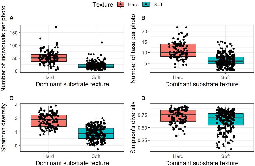
Almond et al. Habitat Heterogeneity and Benthic Biodiversity in the PGC
TABLE 2 | Mean % cover per photo of substrate size classifications by region/depth set.
Region Depth (m) Benthic substrate
Mud Sand Gravel Pebbles Cobbles Boulders Bedrock Biogenic
Duse Bay 200 86.1 4.0 2.3 1.3 0.1 0.4 0 5.8
Duse Bay 300 98.4 0 0 0.1 0.1 0.4 0 1.4
Duse Bay 400 98.9 0 0.4 0 0 0 0 0.6
Duse Bay 500 99.0 0 0 0.2 0 0 0 0.9
PGC-S 200 0 6.7 48.1 5.5 1.3 2.1 19.3 16.7
PGC-S 500 22.1 0.6 38.4 15.1 1.9 3.6 8.0 9.2
PGC-S 800 0.8 0.8 68.4 5.1 0.8 0.6 18.9 4.5
PGC-M 850 29.2 0 0 61.3 1.4 2.0 0.1 5.9
Cape Obelisk 400 90.3 0 0.5 0.7 0.3 1.3 0 7.3
Cape Obelisk 500 91.8 0 1.3 1.4 0.9 0.3 0 4.5
Cape Obelisk 800 92.1 0 0.4 1.0 0.3 0.4 3.2 2.5
Andersson Island 500 96.2 0 0 0 0 0 0 3.7
Biogenic cover accounts for bioconstructors which act as habitat-forming substrate, including Porifera, tube forming Polychaeta, Bryozoa, and Anthozoa. PGC, Prince Gustav Channel;
S, South; M, Mid.
hydrozoans, and poriferans were underrepresented in the AGT on hard substrata, while there was no significance in Simpson’s
catch, while bivalves, holothurians, echinoids, and hemichordates diversity between textures (Figure 4). This suggests that diversity
were underrepresented in the SUCS. In total 11 VME taxonomic in the sense of species richness and evenness of those species was
categories were observed from SUCS imagery and 13 from the greater on hard habitats, there was little change in the dominance
AGT. Several VME taxa were absent from the SUCS imagery, of relative taxa between the two.
including brachiopods, chemosynthetic species (e.g., decapods, Region and substrate texture appeared to have a greater role
bivalves, and tubeworms), acorn barnacles, stalked crinoids, in determining benthic community composition along CA1 than
basket stars, and the scallop Adamussium colbecki. Brachiopods depth while CA2 appeared to be more related to depth (Figure 5).
and acorn barnacles were present, but rare, in the AGT sample. The first two axes of the CA explained 45% of the observed
VME abundance varied significantly between sites (Table 4). The variation (CA1 = 36% and CA2 = 9%). The Andersson Island
highest abundances of VME taxa were found at PGC South and Duse Bay communities show greater variation along CA1
and Mid, with its peak at PGC South 200 m (33.17 ± 12.18), compared to the other regions. The majority of the CA1 scores
while the lowest abundances were at Duse Bay 400 and 500 m for Andersson Island and Duse Bay were negative. Cape Obelisk,
(1.47 ± 1.59 and 1.93 ± 3.86, respectively). VME biomass was PGC South, and PGC Mid all had positive CA1 scores except for
also greatest at PGC South, with a combined total of 30.07 kg only a few samples (Figure 5). Substrate texture also appeared
across the three sampled depths. VME biomass was dominated to be important along CA1 as the hard substrate scores were all
by Porifera in both the AGT and SUCS samples, accounting for positive, apart from four images, while the soft substrate sites
73.64 and 42.52% of biomass, respectively. For 10 out of the 12 were distributed along the entire CA1 axis. The variability in
sampled sites, estimated VME biomass over 1200 m2 exceeded CA2 scores increased with increasing CA1 scores. The majority
the 10 kg threshold set out by CCAMLR to define a VME Risk of CA2 scores for Cape Obelisk were positive except for a few
Area (Table 5). samples. This was the opposite for PGC South and PGC Mid.
From the SUCS imagery alone, benthic community structure There appeared to be some relationship between CA2 scores and
varied greatly between regions (Figure 3), and there were depth, albeit weak. The majority of samples taken at 200 and
significant differences in the numbers of organisms observed 850 m had negative CA2 scores, while those sampled at 400 and
between deployment sites (Table 4). PGC South had the highest 800 m had mainly positive CA2 scores.
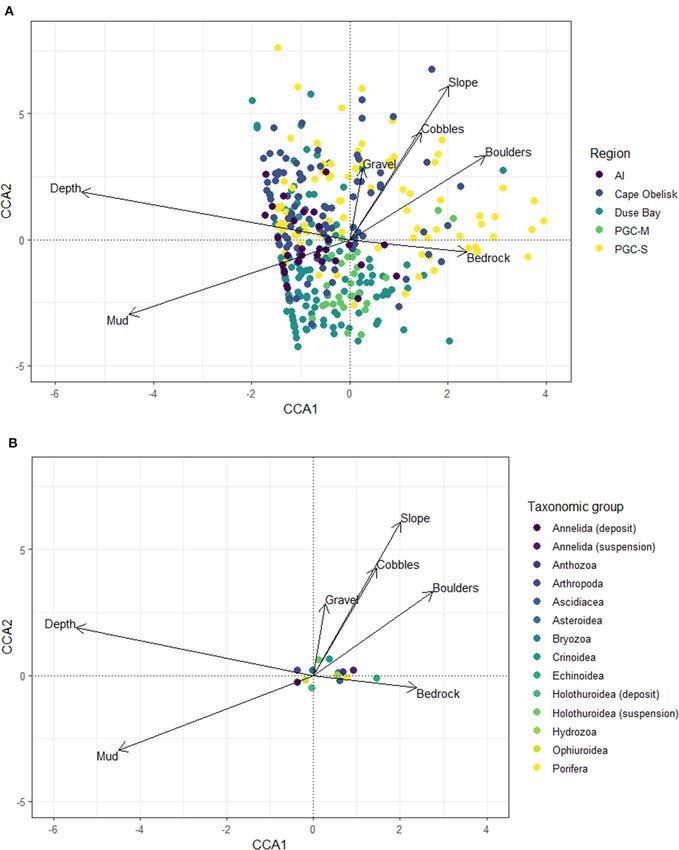
mean numbers of individuals per photo at its three sampled Substrate cover, slope angle, and depth together accounted
depths (65.32 ± 19.22, 58.97 ± 17.39, and 56.38 ± 17.39 at 800, for 52% of variation observed in the CCA which was related to
500, and 200 m, respectively). The PGC Mid 850 m site contained benthic community composition of the SUCS images (Figure 6).
an average of 39.93 ± 9.66 individuals per photo, while all other High variance inflation factors (>10) were observed for slope
regions had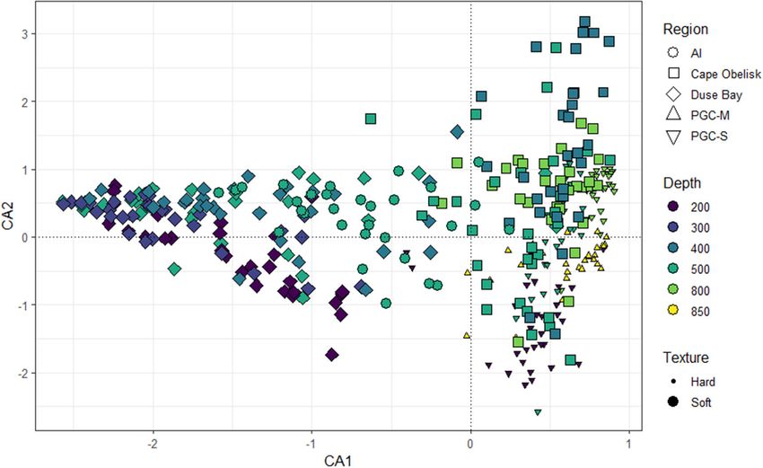
Almond et al. Habitat Heterogeneity and Benthic Biodiversity in the PGC
TABLE 3 | All taxa observed and identified from SUCS imagery and AGT, including relative proportion of total observation/catch.
Phyla Taxa SUCS AGT
Total counted % of total Total counted % of total
Annelida Polychaeta 220 1.93 329 6.15
Clitellata 0 0 2 0.04
Arthropoda Decapoda 214 1.88 39 0.73
Euphausiacea 0 0 3 0.06
Amphipoda 170 1.49 83 1.55
Isopoda 4 0.04 31 0.58
Mysidacea 645 5.65 20 0.37
Pycnogonida 1768 15.51 954 17.83
Brachiopoda Brachiopoda 0 0 4 0.07
Bryozoa Bryozoans 567 4.98 17 0.32
Cephalorhyncha Cephalorhyncha 0 0 9 0.17
Chordata Actinopterygii 50 0.44 8 0.15
Ascidiacea 453 3.98 120 2.24
Cnidaria Actiniaria 27 0.24 28 0.52
Alcyonacea 544 4.77 25 0.47
Pennatulacea 9 0.08 1 0.02
Scleractinia 14 0.12 0 0
Hydroidozoa 649 5.69 75 1.40
Echinodermata Asteroidea 39 0.34 32 0.60
Crinoidea 95 0.83 22 0.41
Echinoidea 118 1.04 466 8.71
Holothuroidea 161 1.41 236 4.41
Ophiuroidea 4630 40.63 1850 34.57
Hemichordata Hemichordata 0 0 500 9.34
Mollusca Bivalvia 0 0 173 3.23
Gastropoda 72 0.63 46 0.86
Scaphopoda 53 0.47 33 0.62
Cephalopoda 1 0.01 0 0
Polyplacophora 0 0 5 0.09
Nemertea Nemertea 0 0 20 0.37
Porifera Porifera 379 3.33 94 1.76
Sipuncula Sipuncula 0 0 5 0.09
Unidentified VME Unidentified VME 514 4.51 121 2.26
Total 11396 5351
strongly associated with an increase in slope gradient and Pycnogonida were also characterized by a very patchy abundance,
hard substrates such as cobbles, boulders and gravel, while reaching their highest abundance at an average of 23.04 ± 8.99
suspension feeding annelids, anthozoans, bryozoans, porifera, per photo, while at most sites this remained below five. Crinoidea
hydrozoans, and ascidians were more closely associated with and Echinoidea were also patchy in abundance, being among the
bedrock (Figure 6B). Deposit feeding annelids, holothurians, few groups to not occur at every site.
and ophiuroids were associated with mud. Abundance varied The SEM investigating the effects of depth, gradient and
significantly for 11 of the 18 identified higher classifications that substrate on CA1 and CA2 score was found to represent the
were tested (Table 4). All 11 saw their peak in abundance within data well (Fisher C = 4.49, p = 0.098, df = 9). There was a
the PGC South region. For Anthozoa, Ascidiacea, Bryozoa, significant indirect pathway between slope gradient and CA1
Echinoidea, Hydroidilina, Porifera, and Scaphopoda this was at score, mediated through its direct influence on substrate cover
200 m, although for the latter this may not be meaningful as (Figure 7; Table 6). The relationship between gradient and hard
Scaphopoda are infaunal so will rarely be identified using SUCS substrate cover was positive while the relationship between
imagery. Crinoidea and Holothuridea were highest in abundance gradient and soft substrate cover was negative. Hard substrate
at 500 m, while Pycnogonida were highest in abundance at 800 m. cover had a positive influence on CA1 score, while soft cover
Frontiers in Marine Science | www.frontiersin.org 7 January 2021 | Volume 8 | Article 614496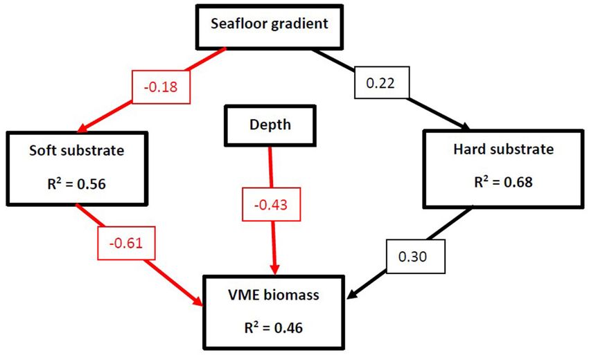
Frontiers in Marine Science | www.frontiersin.org

                                                                                                                                                                                                                                                                                                Almond et al.
                                                    TABLE 4 | Mean number of individuals identified at each location in the Prince Gustav Channel.

                                                    Region                                          Duse Bay                                                       PGC-S                              PGC-M                           Cape Obelisk                       Anderson Island

                                                    Depth (m)                200              300              400              500                200               500               800               850              400               500              800                 500

                                                    Taxa
                                                    Actinopterygii      0.12 ± 1.19        0.08 ± 1       0.07 ± 0.09       0.03 ± 0.08        0.72 ± 1.1       0.65 ± 1.12        0.69 ± 1.29      0.07 ± 0.74       0.59 ± 0.99       0.2 ± 1.51       0.07 ± 0.33         0.2 ± 0.47
                                                    Amphipoda           0.52 ± 1.16       0.9 ± 1.14      0.43 ± 0.67       0.27 ± 0.44       1.31 ± 1.34       0.73 ± 1.03        0.2 ± 0.49       0.62 ± 0.81       0.3 ± 0.59       0.31 ± 0.59        0.2 ± 0.6          0.1 ± 0.21
                                                    Annelida            0.21 ± 0.55       0.33 ± 1.45     0.17 ± 0.45       0.07 ± 0.12       2.28 ± 3.41       1.67 ± 1.51        0.2 ± 0.49       0.55 ± 0.67       0.97 ± 0.98      0.48 ± 0.81       0.47 ± 1.15         0.13 ± 0.34
                                                    Anthozoa              1.72 ± 1        0.17 ± 0.37      0.23 ± 0.5       0.27 ± 0.51       7.86 ± 7.56       3.93 ± 3.16         2 ± 3.61        1.38 ± 1.19       1.73 ± 1.05      1.24 ± 1.87       0.63 ± 1.25         0.37 ± 0.66
                                                    Ascidiacea          3.72 ± 7.65       0.77 ± 1.82     0.13 ± 0.43        0.6 ± 2.3         4.1 ± 5.38        1.8 ± 2.33        0.56 ± 1.3       1.14 ± 1.91       0.77 ± 1.26      0.59 ± 0.62       0.83 ± 1.95         0.33 ± 0.94
                                                    Asteroidea          0.03 ± 0.18       0.07 ± 0.25     0.07 ± 0.25       0.03 ± 0.18       0.17 ± 0.32        0.2 ± 0.54        0.12 ± 0.32      0.17 ± 0.46       0.13 ± 0.34      0.17 ± 0.73       0.07 ± 0.25         0.07 ± 0.25
                                                    Bryozoa               2.69 ± 3        1.47 ± 1.76     0.17 ± 0.45       0.23 ± 0.67       5.07 ± 4.25        4.7 ± 3.62        1.28 ± 2.66      1.59 ± 1.59       1.23 ± 2.03      0.59 ± 1.08       0.57 ± 1.87         0.5 ± 0.92
                                                    Crinoidea               0±0              0±0              0±0               0±0           0.59 ± 1.03        1.3 ± 1.39        0.08 ± 0.27          0±0           0.67 ± 1.11      0.51 ± 0.72       0.03 ± 0.07            0±0
                                                    Decapoda              1 ± 1.46        1.47 ± 1.41      0.7 ± 0.94       0.73 ± 0.85       1.14 ± 0.34        0.5 ± 0.76         0.2 ± 0.4       0.27 ± 0.25       0.8 ± 0.83       0.83 ± 1.24        0.2 ± 0.4          0.57 ± 0.8
                                                    Echinoidea              0±0              0±0              0±0               0±0            2.9 ± 3.94        0.4 ± 1.17           0±0           0.38 ± 0.61        0.2 ± 0.4       0.03 ± 0.18          0±0                 0±0
                                                    Gastropoda          0.01 ± 0.12       0.03 ± 0.09     0.03 ± 0.18       0.01 ± 0.11       0.69 ± 1.39        0.9 ± 1.07        0.88 ± 1.18      0.03 ± 0.18       0.03 ± 0.1       0.04 ± 0.09        0.03 ± 1           0.07 ± 0.11
                                                    Holothuroidea       0.24 ± 0.82       0.3 ± 0.64        0.1 ± 0.3       0.07 ± 0.25        0.52 ± 1.1       2.13 ± 3.39        0.52 ± 0.59      1.17 ± 1.26       0.43 ± 0.99        0.1 ± 0.3       0.23 ± 0.42         0.03 ± 0.17
                                                    Hydroidilina        1.09 ± 1.14       0.53 ± 0.88      0.7 ± 0.97        0.7 ± 1.13       7.34 ± 8.24        3.9 ± 3.13        2.12 ± 3.52      2.03 ± 1.38       1.17 ± 1.04      0.52 ± 0.67       0.7 ± 0.86          0.9 ± 1.19
                                                    Mysida              0.93 ± 1.11       0.7 ± 0.86       2.4 ± 1.89        1.9 ± 1.76       2.69 ± 1.74       3.23 ± 2.25        0.72 ± 1.04      0.38 ± 0.72       1.5 ± 1.31       1.34 ± 1.11       3.2 ± 2.23          2.77 ± 1.41
                                                    Ophiuroidea        15.28 ± 9.75      17.27 ± 8.84     7.17 ± 4.27       10.9 ± 9.23      11.62 ± 10.96      11.47 ± 5.44     30.56 ± 11.53 24.17 ± 8.86           9.73 ± 6.81      2.93 ± 2.48       8.13 ± 5.64         9.1 ± 3.76
                                                    Porifera            1.62 ± 2.96       0.43 ± 0.88       0.1 ± 0.4       0.13 ± 0.42       4.97 ± 4.84       1.97 ± 2.83        0.52 ± 1.14      1.55 ± 1.35       0.33 ± 0.6       0.55 ± 0.88       0.27 ± 0.63         0.3 ± 0.53
8

                                                    Pycnogonida          0.34 ± 0.6       0.5 ± 0.85        5.2 ± 1.3       0.77 ± 0.96           0±0           15.53 ± 9.17      23.04 ± 8.99      1.72 ± 2.29       5.2 ± 3.38       2.66 ± 3.05       8.47 ± 4.89         2.57 ± 1.99
                                                    Scaphopoda              0±0              0±0              0±0               0±0           0.31 ± 0.59       0.67 ± 1.04        0.88 ± 0.77      0.07 ± 0.25          0±0               0±0              0±0                 0±0
                                                    VME                10.24 ± 15.16      2.63 ± 3.57     1.47 ± 1.59       1.93 ± 3.86      33.17 ± 12.18      19.5 ± 12.8       8.24 ± 12.18     10.59 ± 4.06       7.67 ± 6.01      5.24 ± 4.43       3.8 ± 6.28          3.17 ± 3.32
                                                    Overall            29.07 ± 23.39      24.3 ± 8.3      13.93 ± 4.67 16.63 ± 10.95 56.38 ± 17.39 58.97 ± 17.39 65.32 ± 19.22 39.93 ± 9.66 27.53 ± 10.13 14.76 ± 6.04 25.07 ± 10.46                                        18.53 ± 5.52

                                                    ANOVA was used to test differences among locations for each taxa with significant (p < 0.05) differences indicated in bold. Taxa with
Almond et al. Habitat Heterogeneity and Benthic Biodiversity in the PGC
TABLE 5 | Estimated VME taxa wet weight over 1200 m2 (kg) using mean weights determined for each taxa from AGT data per SUCS deployment site.
Region Depth (m) VME Taxa
Ascidacea Bryozoa Cidaroidea Cnidaria Porifera Polychaeta, Serpulidae Unidentified VME Total
Duse Bay 200 20.35 12.65 0.50 11.91 106.86 0 0.53 152.84
Duse Bay 300 9.13 1.91 0 4.70 45.80 0 1.07 62.61
Duse Bay 400 1.66 0.59 0 25.50 15.27 0 2.14 25.50
Duse Bay 500 1.67 0.59 0 3.25 3.56 0 0 9.06
PGC-S 200 137.02 8.53 0 46 178.1 1.38 45.44 416.45
PGC-S 500 107.95 7.94 0 66.54 137.39 2.99 50.25 373.06
PGC-S 800 79.72 6.18 0 36.83 103.81 1.44 28.22 256.20
PGC-M 850 79.89 4.18 0 24.67 125.29 0 30.41 264.45
Cape Obelisk 400 15.78 5.44 0.54 33.29 14.25 1.49 50.23 108.74
Cape Obelisk 500 8.30 2.50 0.27 17.37 25.44 1.10 27.80 82.78
Cape Obelisk 800 7.89 0.74 0 5.25 8.65 1.70 1.60 25.82
Andersson Island 500 1.66 2.21 0 1.50 3.05 0 1.07 9.49
Red totals exceed CCAMLR’s guidelines of 10 kg per 1200 m2 longline haul, suggesting they should be classified as VME high risk areas. PGC, Prince Gustav Channel; S, South;
M, Mid.
to biogenic substrate cover. The cover of biogenic substrate
had a direct negative influence on CA2. The CA2 scores likely
represent a gradient of biogenic cover and depth. This suggests
that some taxa are potentially physiologically depth limited, or
an unmeasured variable is mediating this process. The SEM
investigating the direct and indirect effects of slope gradient,
depth, and substrate cover on VME biomass was a good fit
for the data (Fisher C = 6.51, P = 0.072, df = 6). Seafloor
gradient had a significant indirect effect on biomass, mediated
through its influence on substrate cover (Figure 8; Table 6).
Gradient had a negative relationship with soft substrate, while
soft substrate had a negative relationship with biomass. The
reverse was true of the relationship between gradient and hard
substrate and between hard substrate and biomass. Cumulatively,
seafloor gradient therefore has a strong, positive relationship with
predicted biomass. Contrary to the predicted outcomes, depth
had a direct, negative influence on biomass. This suggests that
some VME taxa observed are either physiologically depth-limited
FIGURE 3 | Examples of in-situ SUCS images of common benthic or influenced by an unmeasured variable that is itself mediated
communities and taxa. (A) Biogenic habitat forming taxa including poriferan by depth. It is also possible the full depth range within the
species and the pencil spine urchin cidaroid, (B) species associated with hard channel has not been adequately sampled to properly identify
substrata including crinoid species, and suspension feeding dendrochirotid
depth trends.
holothurians, cnidarians, and annelids, (C) ophiuroid dominated community
(cf. Ophionotus victoriae), and (D) deposit feeding holothurian Protelpidia
murrayi in a mud dominated area. Scale bars represent 10 cm.
DISCUSSION
Our work found that benthic faunal composition was heavily
had a negative one. This suggests that the CA1 scores represent a influenced by the substrate type available, with greater
gradient of soft to hard substrate that is influencing community abundances and diversity associated with hard, rocky substrate.
structure, while depth does play a smaller yet still significant role. This was often associated with the physiology and functional
Contrary to what was expected, a significant direct association group of different taxa. Depth and seafloor gradient had direct
between seafloor gradient and CA2 score was found. This and indirect effects on community structure, often mediated
suggests seafloor gradient is influencing community structure via through their influence on habitat forming organisms and
a different unmeasured variable. Depth had no association with substrate type. High numbers of VME taxa were identified, and
abiotic substrate cover. Depth did have a positive direct influence VME biomass was strongly associated with hard substrate and
on CA1 and a greater influence on CA2 but was negatively related shallower depths.
Frontiers in Marine Science | www.frontiersin.org 9 January 2021 | Volume 8 | Article 614496Almond et al. Habitat Heterogeneity and Benthic Biodiversity in the PGC FIGURE 4 | Mean number of individuals and taxa present per SUCS image and mean diversity indices per photo according to substrate texture. (A) Mean number of individuals per image, (B) Mean number of taxa per image, (C) Mean diversity (Shannon-Weiner Index), and (D) Mean diversity (Simpson’s Index). FIGURE 5 | Correspondence Analysis (CA) of benthic community structure according to region, depth, and substrate texture. CA1 and CA2 axis together explain 45% of observed variation. Benthic Assemblages and Physical Substrate texture and type in particular have been found to Variables play significant roles in structuring epifaunal communities in The influence of physical environmental variables such as other regions around the Antarctic Peninsula, including the substrate type, substrate texture, and depth have frequently South Orkney Islands and King George Island (Quartino et al., been associated with the distribution and structure of benthic 2001; Brasier et al., 2018). Similar results have been found in communities around the Antarctic continental shelf and slope. east Antarctica (Post et al., 2011) and in the Ross Sea, where Frontiers in Marine Science | www.frontiersin.org 10 January 2021 | Volume 8 | Article 614496
Almond et al.                                                                                           Habitat Heterogeneity and Benthic Biodiversity in the PGC

 FIGURE 6 | Canonical Correspondence Analysis (CCA) of community assemblage and environmental variables including substrate cover, depth, and seafloor slope
 gradient. Organisms are grouped into higher taxonomic classifications and functional groups were necessary. (A) Site scores. (B) Taxon scores.

substrate type and composition explained 66% of the variation                      Conversely, finer, siltier sediments provide a food resource for
observed in shallow water macrofaunal communities (Cummings                        both facultative and obligate deposit feeders (Gutt, 1990). This
et al., 2006). Coarse substrates are preferential for most filter                  is reflected in the PGC, where deposit feeding holothurians
or suspension feeders, as it often provides hard surface for                       and annelids were strongly associated with muddy sediments.
attachment and an elevated position which enhances the capture                     Although, it is likely that the diversity and abundance of these
success rate of these functional groups (Muschenheim, 1987).                       taxonomic groups will be underestimated because the analysis

Frontiers in Marine Science | www.frontiersin.org                             11                                        January 2021 | Volume 8 | Article 614496
Almond et al.                                                                                                  Habitat Heterogeneity and Benthic Biodiversity in the PGC

 FIGURE 7 | Structural equational model (SEM) exploring the relationships between seafloor gradient, depth, substrate cover, and community structure as measured
 by CA1 and CA2 axis scores. Arrows represent unidirectional relationships among variables, with black arrows denoting positive relationships and red arrows
 depicting negative ones. Only significant pathways (P ≤ 0.05) are displayed. The standardized regression coefficient is given in the associated box. R2 s for component
 models are given in the boxes of the response variable. Model incorporates random effect of Region. Hard substrate represents the combined cover of gravel,
 cobbles, pebbles, boulders, and bedrock. Soft substrate represents the combined cover of sand and mud.

is based on images of the benthic communities rather than a                             and hard substrates likely has a cumulative effect on the diversity
combination of infaunal and epifaunal sampling. Suspension                              of these assemblages. High diversity and abundance of taxa found
feeders such as some cnidarians and crinoids were associated with                       on hard substrates is enhanced by the three-dimensional surface
rocky habitats. As in this present study, abundance, biomass, and                       created by the organisms themselves, particularly Porifera,
taxonomic epifaunal diversity are often found to be greater in                          some anthozoans, and bryozoans, which form complex habitats
areas of coarse, hard substrates than in areas of finer sediments.                      for other invertebrates. This is reflected in the SEM which
This was the case in east Antarctica, where boulders and cobbles                        suggests biogenic cover played a significant role in determining
were associated with significant increases in faunal abundance                          overall community structure. Other studies have noted the
(Post et al., 2017) and in deeper communities (c. 1000 m) in the                        positive correlations between overall abundance and diversity
Weddell Sea (Jones et al., 2007).                                                       and the presence of ecosystem engineers such as large sponges,
   It has been suggested that differences in diversity could be                         gorgonians, and bryozoans (Gutt and Shickan, 1998; Gutt and
related to the abundance of suspension feeding taxa that prefer                         Starmans, 1998). It is also possible that limitations inherent in
hard substrates being highly diverse in Antarctic waters (Gutt and                      the SUCS imagery means biodiversity in soft sediment areas
Starmans, 1998). The resolution of taxonomic data available from                        cannot be reliably estimated. Epifauna that periodically burrow
SUCS imagery prevents analysis of the exact number of epifaunal                         and infauna will be underestimated or not observed using SUCS
species present, but greater diversity amongst hard substrates of                       imagery. This may explain the observed underrepresentation
deep water corals has been found off the Antarctic Peninsula                            of bivalves, hemichordates, echinoids, and holothurians in the
when identified to genus level (Roberts and Hirshfield, 2004).                          SUCS data compared to the AGT data. Previous studies have
In the PGC, those areas dominated by harder substrates were                             noted higher than expected levels of diversity among infaunal
also characterized by increased habitat heterogeneity. The higher                       communities in soft sediment areas, including in the South
diversity observed at these sites may therefore be a result of fauna                    Shetland Islands and the Antarctic shelf in general (Gallardo,
characteristic of both coarse and fine sediment being able to                           1987; Lovell and Trego, 2003). It is possible that this may be
occupy the same space, as more ecological niches and functional                         the case in the PGC. However, this cannot be confirmed in the
groups are provided for. The association of sessile invertebrates                       present study.

Frontiers in Marine Science | www.frontiersin.org                                  12                                           January 2021 | Volume 8 | Article 614496
Almond et al.                                                                                                        Habitat Heterogeneity and Benthic Biodiversity in the PGC

TABLE 6 | Summary of all direct pathways investigated using structural equation models and the hypothesis underpinning the expected relationship between predictor
and response variables.

Predictor variable         Response variable           Hypothesis                                                        Outcome                                Standardized
                                                                                                                                                                 regression
                                                                                                                                                                 coefficient

Depth                      Biogenic cover              Depth will have no direct significant impact on                   Increase in depth = decrease in            −0.44
                                                       community structure (Dayton et al., 1982)                         cover of biogenic substrate
                           Hard substrate              Depth will have no direct significant impact on substrate         No direct significant pathway                -
                                                       cover
                           Soft substrate              Depth will have no direct significant impact on substrate         No direct significant pathway                -
                                                       cover
                           CA1 score                   Depth will have no direct significant impact on                   Increase in depth = increase in            0.12
                                                       community structure (Dayton et al., 1982)                         CA1 score
                           CA2 score                   Depth will have no direct significant impact on                   Increase in depth = increase in            0.23
                                                       community structure (Dayton et al., 1982)                         CA2 score
                           VME biomass                 Depth will have no direct significant impact on                   Increase in depth = decrease in            −0.43
                                                       community structure (Dayton et al., 1982)                         VME biomass
Seafloor gradient          Biogenic cover              Seafloor gradient will have no direct significant impact on       No direct significant pathway                -
                                                       community structure
                           Hard substrate              Seafloor gradient will affect sedimentation rates, with           Increase in slope                          0.22
                                                       lower gradients resulting in greater cover of soft, fine          gradient = increase in rocky
                                                       sediments (Post et al., 2020)                                     substrate cover
                           Soft substrate              Seafloor gradient will affect sedimentation rates, with           Increase in slope                          −0.18
                                                       lower gradients resulting in greater cover of soft, fine          gradient = decrease in mud
                                                       sediments (Post et al., 2020)                                     cover
                           CA1 score                   Seafloor gradient will have no direct significant impact on       No direct significant pathway                -
                                                       community structure
                           CA2 score                   Seafloor gradient will have no direct significant impact on       Increase in slope                          0.19
                                                       community structure                                               gradient = increase in CA2 score
                           VME biomass                 Seafloor gradient will have no direct significant impact on       No direct significant pathway                -
                                                       community structure, and therefore VME biomass
Biogenic cover             CA1 score                   Biogenic cover will significantly affect community                No direct significant pathway                -
                                                       structure due to the role of bioconstructors in creating
                                                       additional habitat (Gutt and Starmans, 1998)
                           CA2 score                   Biogenic cover will significantly affect community                Increase in cover of biogenic              −0.34
                                                       structure due to the role of bioconstructors in creating          substrate = decrease in CA2
                                                       additional habitat (Gutt and Starmans, 1998)                      score
Hard substrate             CA1 score                   Substrate type will significantly affect community                Increase in rocky substrate                0.22
                                                       composition (Post et al., 2017)                                   cover = increase in CA1 score
                           CA2 score                   Substrate type will significantly affect community                No direct significant pathway                -
                                                       composition (Post et al., 2017)
                           Biogenic cover              Substrate type will significantly affect community                Increase in hard substrate                 0.21
                                                       composition (Post et al., 2017)                                   cover = increase in biogenic
                                                                                                                         cover
                           VME biomass                 An increase in rocky cover will result in greater VME             Increase in rocky substrate                 0.3
                                                       biomass (Brasier et al., 2018)                                    cover = increase in VME
                                                                                                                         biomass
Soft substrate             CA1 score                   Substrate type will significantly affect community                Increase in mud                            −0.3
                                                       composition (Post et al., 2017)                                   cover = decrease in CA1 score
                           CA2 score                   Substrate type will significantly affect community                No direct significant pathway                -
                                                       composition (Post et al., 2017)
                           VME biomass                 An increase in mud cover will result in a decrease in VME         Increase in mud                            −0.61
                                                       biomass (Brasier et al., 2018)                                    cover = decrease in VME
                                                                                                                         biomass

Regression coefficients were standardized using scaling by standard deviation. CA1 and CA2 axis scores act as a proxy for community structure.

   Community composition was influenced by depth and                                        Starmans (1998) found that some variation in the benthos could
seafloor gradient in the PGC, albeit not as significantly as                                be explained by a combination of these two factors. While several
substrate type and often through indirect effects. Gutt and                                 studies have highlighted the role of depth in determining benthic

Frontiers in Marine Science | www.frontiersin.org                                      13                                             January 2021 | Volume 8 | Article 614496
Almond et al. Habitat Heterogeneity and Benthic Biodiversity in the PGC
FIGURE 8 | Structural equational model (SEM) exploring the relationships between slope angle, depth, substrate cover, and estimated VME biomass. Arrows
represent unidirectional relationships among variables, with black arrows denoting positive relationships and red arrows depicting negative ones. Only significant
pathways (P ≤ 0.05) are displayed. The standardized regression coefficient is given in the associated box. R2 s for component models are given in the boxes of the
response variable. Model incorporates random effect of Region. Hard substrate represents the combined cover of gravel, cobbles, pebbles, boulders, and bedrock.
Soft substrate represents the combined cover of sand and mud.
composition (Post et al., 2017; Neal et al., 2018), others suggest consider variations in the small-scale also often result in stronger
that the influence of depth is either non-existent or limited to distinctions between assemblages than those that use larger
indirectly effecting the benthos through its mediating impact on geomorphic units (Douglass et al., 2014; Brasier et al., 2018).
other physical variables (Brandt et al., 2007; Jones et al., 2007). Gutt et al. (2012) argue that broad patterns in environmental
After the mass-wasting of benthic communities caused during variables can be used to explain variation at larger scales (>2 km),
the Cenozoic glacial period, it is thought that the continental shelf whereas fewer variables explain variation at finer scales. These
was predominantly recolonised by deep-water organisms with variations are likely explained by non-measured variables as
wide bathymetric tolerances (Thatje et al., 2005). This legacy is well as biological interactions and traits. The influence of small-
still evident today, and as a result depth is typically regarded as scale heterogeneity in determining community composition,
less important in controlling species distributions than in many particularly in areas dominated by muddy sediments, is evident
other areas (Dayton et al., 1982). Thus, any direct change in in this study. Dropstones in particular are a noted small-scale
abundance and diversity with depth is likely related to a reduction physical feature that act as important habitats and enhance
in organic matter available to the benthos (Lampitt et al., 2001). diversity among sessile invertebrates in both the Antarctic
The influence of seafloor gradient on the benthos has not been as and Arctic (Thrush et al., 2010). It has been suggested that
thoroughly studied, although in this present study its influence dropstones act as important stepping stones for the dispersal
was limited to its effect on substrate cover. Flatter gradients result and connectivity of communities that rely on hard substrates
in greater sedimentation accumulation and the dominance of fine (Post et al., 2017), and given that most of the Antarctic shelf
sediments (Post et al., 2020), as evidenced in the present study is dominated by muddy sediments (Smith et al., 2006), their
through the high inflation factors between gradient and some potential importance for the overall biodiversity of a system
hard substrates, which will in turn influence both the texture of cannot be underestimated. A higher level of connectivity between
the habitat and the accumulation of particulate matter available hard substrate-preferring taxa may also be reflected in the PGC
for deposit feeders. data, evidenced by the high levels of similarity between the
The relative influence of physical environmental variables communities found at PGC South and Mid, especially when
depends on the scale of investigation. Previous studies of the compared to the soft sites of Duse Bay and Cape Obelisk,
Antarctic shelf have highlighted the problems associated with which despite sharing similar sediment characteristics supported
using large-scale, regional patterns to predict benthic abundance different communities. This suggests small scale heterogeneity
and distribution. Variations in habitat and substrate on the is particularly important in muddy, soft sedimented habitats
local, often sub-meter, scale have significant impacts on overall where local variation can greatly impact benthic abundance
diversity (Cummings et al., 2006; Post et al., 2017). Studies that and diversity.
Frontiers in Marine Science | www.frontiersin.org 14 January 2021 | Volume 8 | Article 614496Almond et al. Habitat Heterogeneity and Benthic Biodiversity in the PGC Changes in annual and seasonal sea ice cover must be (Sumida et al., 2008; Grange and Smith, 2013). Abundance was considered when investigating benthic community structure. however lower than in the Weddell Sea shelf (Gutt and Starmans, In the eastern Weddell Sea, benthic abundance, and biomass 1998). It is likely that the full extent of benthic distribution decreased by up to two thirds and composition shifted from and diversity cannot be assessed completely. More AGTs would suspension to deposit feeders as a result of sea ice increases be necessary so that the sample size is meaningful enough to between 1988 and 2014 (Pineda-Metz et al., 2020). In the present carry out more robust analysis on the catch data. The SUCS also study, the communities found occupying all depths at Cape has some inherent limitations. The SUCS is a downward facing Obelisk were distinctly unique from the communities found camera, meaning it can only land on flat surfaces. This prevents elsewhere in the PGC. It is possible that the communities certain regions such as steep slopes, boulders, and canyons from here are still experiencing the legacy of the Prince Gustav ice being studied due to their topography. These habitats are often shelf, which permanently covered Cape Obelisk as recently as considered diversity hotspots (Robert et al., 2015; Fernandez- 1989 (Cooper, 1997). Fauna characteristic of a system that has Arcaya et al., 2017), meaning these potentially diverse regions are undergone change from an oligotrophic sub-ice shelf ecosystem difficult to sample. to a productive shelf ecosystem are often unique to these systems, and it has been suggested that some benthic communities can VME Taxa take 150–200 years to reach complete recolonization following The relationship between benthic community composition and exposure to the sea surface (Gutt et al., 2010). These fauna can environmental characteristics is complex with many variables vary from pioneer organisms such as demosponges and juvenile contributing to differences in community composition and the cnidaria to taxa more typical of advanced stages of recolonization spatial structure of biodiversity (Convey et al., 2014). Given the such as sponges, compound ascidians, and unique bryozoans. current international effort to establish a representative system While higher numbers of ascidians and porifera were found at of MPAs in the Southern Ocean it is important to continue to Cape Obelisk compared to its muddy counterparts, resolution of investigate the relationship between both broad and local scale the SUCS imagery and the lack of AGT data from this region physical surrogates that could be used to infer high levels of prevents analysis down to species level. biodiversity, VME locations, and potential MPA sites. The range and distribution patterns of different taxa are highly Abundances of VME taxa were greatest within the PGC dependent on both life history and evolutionary history (Barnes South sites, and VME biomass was characterized by an increase and Griffiths, 2007; Convey et al., 2014). Some groups, such association with rocky cover and a decrease with mud cover. This as pycnogonids, show a global hotspot of biodiversity within is unsurprising because of the high number of hard substrate- the Southern Ocean, and when examined on a regional scale preferring suspension and filter feeders that are classified as have distinct local hotspots (Griffiths et al., 2011). This was VME taxa (CCAMLR, 2009b). VMEs have been found in lower observed at PGC South 800 m, where their abundance reached abundances on soft sediment compared to hard elsewhere around a significant peak. Polychaetes, similar to pycnogonids, are the Antarctic Peninsula (Lockhart and Jones, 2008; Brasier et al., represented at higher than average levels in Antarctica (Barnes 2018). Depth had a negative influence on VME biomass, which and Peck, 2008). At the South Shetlands Islands, polychaetes is likely related to organic flux and food availability due to the were found to compose up to 61% of the total macrobenthic functional nature of many VME taxa (Jansen et al., 2018). Slope abundance (Gutt and Starmans, 1998). Polychaetes were also gradient played an indirect role in influencing biomass, mediated among the predominating organisms at King George Island through its effect on substrate cover. While the SEM presented in (Arnaud et al., 1986), and despite also being located around the present study may be useful in predicting biomass in specific the Antarctic Peninsula, these patterns were not reflected in regions, the overall impact of variables on VME taxa will likely the PGC, where polychaete abundance remained relatively be highly area specific (Parker and Bowden, 2010). More data are low throughout. However, this is reflective of the individuals required on the relationship between seafloor gradient and VME observed on the seafloor and infaunal samples may provide taxa in order to check the validity of this model for other regions a different perspective. Ophiuroids were the most dominant of the Antarctic shelf and continental slope. taxa found across all sites and among both substrate types. VME Risk Area thresholds are projected to have been met in This has been observed around much of the Antarctic shelf. all sites with the exceptions of Andersson Island and Duse Bay In east Antarctica, ophiuroids represent high proportions of 500 m. The projected wet weights over 1200 m2 in the current overall observed taxa, sometimes up to 50% (Post et al., 2017), study may have implications for the development of future although the proportional abundance of ophiuroids is greater conservation measures across the Antarctic Peninsula as a whole in this current study than in others that have occurred around and the PGC in particular. Several previous studies have provided the Peninsula (Grange and Smith, 2013; Brasier et al., 2018). evidence of VME thresholds being met in the northwestern This dominance is unsurprising, as ophiuroids, as well as Antarctic Peninsula region (Lockhart and Jones, 2008; Parker other echinoderms such as echinoids, are generally considered and Bowden, 2010), which have led to the notification and ubiquitous in the Southern Ocean and can thrive across large designation of new VME Risk Areas by CCAMLR. As in the depth ranges and on both hard and soft substrate (Thrush et al., present study, VME biomass is often driven by porifera, and in 2006). Overall abundance per m2 was greater in the PGC than in some cases the wet weight of porifera alone has been enough to many similar studies around the Antarctic shelf and continental exceed thresholds and make areas high risk (Brasier et al., 2018). slope (Table 7), including the Antarctic Peninsula shelf and fjords This threshold may therefore be severely biased toward “heavy” Frontiers in Marine Science | www.frontiersin.org 15 January 2021 | Volume 8 | Article 614496
You can also read