A minimal model for wind- and mixing-driven overturning: threshold behavior for both driving mechanisms - Potsdam Institute for Climate ...
←
→
Page content transcription
If your browser does not render page correctly, please read the page content below
Clim Dyn (2012) 38:239–260
DOI 10.1007/s00382-011-1003-7

A minimal model for wind- and mixing-driven overturning:
threshold behavior for both driving mechanisms
Johannes J. Fürst • Anders Levermann

Received: 3 July 2010 / Accepted: 20 January 2011 / Published online: 12 February 2011
 Springer-Verlag 2011

Abstract We present a minimal conceptual model for the                 paradigm for the qualitative behaviour of the Atlantic
Atlantic meridional overturning circulation which incorpo-             overturning in the discussion of driving mechanisms.
rates the advection of salinity and the basic dynamics of the
oceanic pycnocline. Four tracer transport processes fol-               Keywords Meridional overturning circulation
lowing Gnanadesikan in Science 283(5410):2077–2079,                    Northern sinking  Critical freshwater threshold
(1999) allow for a dynamical adjustment of the oceanic                 Overturning sensitivity  Conceptual model
pycnocline which defines the vertical extent of a mid-lati-            Stability  Atlantic meridional overturning circulation
tudinal box. At the same time the model captures the salt-             Pycnocline depth  Driving mechanism
advection feedback (Stommel in Tellus 13(2):224–230,
(1961)). Due to its simplicity the model can be solved ana-
lytically in the purely wind- and purely mixing-driven cases.          1 Introduction
We find the possibility of abrupt transition in response to
surface freshwater forcing in both cases even though the               The Atlantic meridional overturning circulation (AMOC),
circulations are very different in physics and geometry. This          a crucial branch of the global oceanic circulation system,
analytical approach also provides expressions for the critical         transports large amounts of heat towards high latitudes. A
freshwater input marking the change in the dynamics of the             cessation of this circulation would reduce temperatures
system. Our analysis shows that including the pycnocline               regionally in the Nordic Seas by up to 8C (Manabe and
dynamics in a salt-advection model causes a decrease in the            Stouffer 1988; Clark et al. 2002) with strong climatic
freshwater sensitivity of its northern sinking up to a                 implications world-wide (Laurian et al. 2009). These
threshold at which the circulation breaks down. Compared to            include changes in precipitation patterns (Vellinga and-
previous studies the model is restricted to the essential              Wood Schmittner 2002), Atlantic ecosystems (Schmittner
ingredients. Still, it exhibits a rich behavior which reaches          2005; Kuhlbrodt et al. 2009), sea level distribution
beyond the scope of this study and might be used as a                  (Levermann et al. 2005; Yin et al. 2009), European climate
                                                                       (Laurian et al. 2010), the El Niño Southern Oscillation
                                                                       (Timmermann et al. 2005) and Asian monsoon systems
J. J. Fürst  A. Levermann                                            (Goswami et al. 2006).
Earth System Analysis, Potsdam Institute for Climate Impact               Since the initial study by Stommel (1961) the discussion
Research and Institute of Physics, Potsdam University, Potsdam,        about past and future variations of the AMOC is linked to
Germany
                                                                       the existence of multiple stable equilibria of the circulation.
e-mail: anders.levermann@pik-potsdam.de
                                                                       Across a large spectrum of climate models, existence of
Present Address:                                                       multiple states has been observed in conceptual models
J. J. Fürst (&)                                                       (Stommel 1961; Johnson et al. 2007; Guan and Huang
Department of Geography and Earth System Sciences,
                                                                       2008), ocean circulation models with idealised geometry
Faculty of Sciences, Vrije Universiteit Brussel, Pleinlaan 2,
Brussels, Belgium                                                      (Marotzke et al. 1988; Marotzke and Willebrand 1991;
e-mail: Johannes.Fuerst@vub.ac.be                                      Thual and McWilliams 1992; Rahmstorf 1995b), various

                                                                                                                           123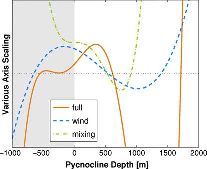
240                                                                           J.J. Fürst, A. Levermann: Minimal overturning model

Earth system Models of Intermediate Complexity (EMICs)           powering the AMOC. In agreement with the results in Park
(Manabe and Stouffer 1988; Rahmstorf et al. 2005; Yin            (1999), the sensitivity of the overturning circulation to
and Stouffer 2007; Ashkenazy and Tziperman 2007) as              freshwater fluxes in the North Atlantic is reduced compared
well as uncoupled oceanic general circulation models             to Stommel (1961). This results from a compensating effect
(Rahmstorf 1996). As state-of-the-art coupled climate            of the pycnocline dynamics that stabelises the overturning.
models are too computationally demanding to explore the             The paper is structured as follows: the model design and
full stability range of their circulation, no multi-stability    its idealised components are presented in Sect. 2. In this
under present day boundary conditions has yet been               context the necessity of tracer advection (see Stommel
observed (Stouffer et al. 2006). Also some models of             (1961)) in the approach of Gnanadesikan (1999) as already
intermediate complexity are reported to lack multi-stability     proposed by Levermann et al. (2005) and Levermann and
of the AMOC (Prange et al. 2003; Nof et al. 2007). In            Fürst (2010) is emphasised. The main results are intro-
these studies, it has been speculated that extensive dia-        duced in Sect. 3, where the model is analysed for three
pycnal mixing might be the reason for multi-stability.           instructive cases. This is followed by an analysis of the
Recently Hofmann and Rahmstorf (2009), showed that               freshwater sensitivity of the northern sinking (Sect. 4) A
multi-stability is possible for a wind-driven overturning.       validation of our conceptual approach is conducted in Sect.
They attributed the existence of multiple stable states to the   5 using the model of intermediate complexity CLIMBER-
Atlantic salinity distribution.                                  3a (Montoya et al. 2005) for a qualitative intercomparison.
   The dispute about the physical mechanism providing the        We conclude in Sect. 6.
necessary energy to sustain an overturning circulation
(Kuhlbrodt et al. 2007) is thus a crucial aspect in the sta-
bility analysis of the AMOC. The two main candidates for         2 Model description
these so-called driving mechanisms are diapyncal mixing
(Jeffreys 1925; Munk and Wunsch 1998; Park 1999) and             For a minimal model that comprises wind- and mixing-
Southern Ocean wind divergence (Toggweiler and Samuels           induced overturning we propose a standard interhemi-
1998; Gnanadesikan et al. 2005). In addition to character-       spheric geometry as illustrated in Fig. 1. It combines the
ising the driving mechanisms of the AMOC, other pro-             four basic meridional tracer transport processes associated
cesses need to be considered for its stability analysis.         with the overturning circulation (Gnanadesikan 1999) and
While surface fluxes of freshwater and heat alone can not        thereby describes changes in the meridional density struc-
sustain a deep overturning circulation (Sandström 1916;         ture. Since we find that changes in heat advection represent
Kuhlbrodt 2010), they are important to set the density           a second order effect compared to salt advection, we keep
structure of the ocean. This density structure determines        oceanic temperatures fixed. This enables analytic solutions
how much of the available energy is indeed directed into a       in a number of cases and captures significant atmospheric
basin wide overturning circulation (Schewe and Lever-            and oceanic feedbacks for the overturning circulation. In
mann 2010). We combine thus the two main driving                 principle the model can be easily generalized to account for
mechanisms of the AMOC with two limiting processes not           the advection of temperature. As surface boundary condi-
providing net energy to the system, but shaping its spatial      tions for salinity we apply constant freshwater fluxes with
pattern following Gnanadesikan (1999). These four pro-           global zero mean. This is represented by two freshwater
cesses are complemented by the advection of salinity and         bridges from the upper mid-latitude box (subscript U) to
thereby a dynamical equation for the meridional density          the southern FS and northern FN box denoted by subscripts
gradient. This is substantial since Levermann and Griesel        S and N, respectively.
(2004) showed that some variations in the Atlantic over-
turning are not captured in Gnanadesikan’s model. So far         2.1 Pycnocline dynamics
an analytically solvable model that comprises both driving
mechanisms of the overturning is missing. In contrast to         The representation of the dynamics of the oceanic pycno-
Johnson et al. (2007) who suggested a similar model, their       cline follows (Gnanadesikan 1999). Here we assume that
focus was to study an inherent oscillation between on- and       the oceanic pycnocline depth D is represented by the ver-
off-state of this circulation. Here we aim to provide a          tical extent of the mid-latitude box. Its time evolution is
minimal model that allows to examine the on-state AMOC           given by four tracer transport processes
stability in a wind- and mixing driven case.                             oD
   Analytical solutions are derived for the purely wind- and     BLU       ¼ mW þ mU  mE  mN :                             ð1Þ
                                                                         ot
the purely mixing-driven circulation cases. Our results
reveal a threshold behaviour with respect to surface fresh-      Here B is the average, zonal extent of the Atlantic ocean
water forcing that is independent of the mechanism               basin, LU is the meridional extent of the tropical boxes

123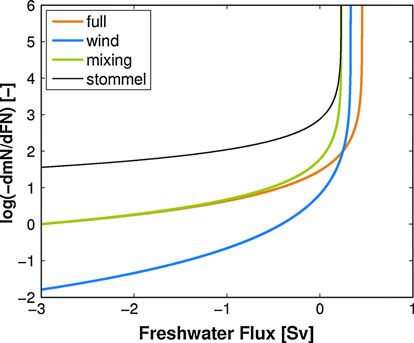
J.J. Fürst, A. Levermann: Minimal overturning model                                                                              241

                                                                           Parameterisations of northern sinking have been derived
                                                                        following numerous approaches summarised in Appendix 1
                                                                        (Robinson 1960; Marotzke 1997; Gnanadesikan 1999;
                                                                        Johnson and Marshall 2002; Guan and Huang 2008). In our
                                                                        model, the scaling is adopted from Marotzke (1997) who
                                                                        assumes a generic density distribution in the Atlantic. This
                                                                        allows to substitute the zonal density difference in the
                                                                        geostrophic equation with a meridional one (Marotzke
Fig. 1 Schematic depiction of the conceptual model. The depth of        1997). A b-plane approximation finally gives
the pycnocline D is determined by the balance between northern deep
water formation mN, mixing driven upwelling in the low latitudes mU,               g Dq 2
Ekman upwelling mW and eddy-induced return flow mE. Salinity is
                                                                        mN ¼ C              D  CN Dq  D2                       ð5Þ
                                                                                 bN LNy q0
advected along with these transport processes and determines together
with a fixed temperature distribution, the density difference between      The constant C is given by the current geometry and
the northern and upper low-latitude box Dq
                                                                        characteristics of the density distribution. Again all
                                                                        quantities except for D and Dq are comprised in a
(between latitudes ±30). Using Ekman boundary layer                    constant CN. We assume that the relevant density
theory, the wind driven volume transport is predicted via a             difference for the northern sinking is to be taken between
scale analysis of the equation of motion.                               the northern and the upper low-latitudinal boxes
            sDr                                                         Dq  qN  qU . This choice represents the most direct
mW ¼ B            ¼ CW                                 ð2Þ
          jfDr jq0                                                      interpretation of the assumptions entering the derivation by
                                                                        Marotzke (1997). In its final form eq. (5) can furthermore
   The mean Coriolis parameter in the Drake passage is fDr
                                                                        be motivated in a more heuristic way: Currently major
while q0 denotes the ocean average density. Wind stress
                                                                        northern sinking occurs in the Nordic Seas. Thus its
feedbacks though possibly relevant (Fyfe et al. 2007;
                                                                        volume transport is mainly defined by the North Atlantic
Toggweiler and Russell 2008) will not be captured by
                                                                        Current crossing the ocean basin from West to East. This
our model. Since there is no dependency on the oceans
                                                                        flow is geostrophically balanced by a meridional difference
density stratification we substitute this flux by a constant
                                                                        in sea surface elevation which is observed in ocean models
CW ¼ mW for simplicity in later calculations. The eddy
                                                                        of varying resolution (Levermann et al. 2005; Landerer
return flow mE is parameterised following Gent and
                                                                        et al. 2007; Vellinga and Wood 2007; Schlesinger et al.
McWilliams (1990) using a thickness diffusivity AGM
                                                                        2006). Due to the existence of a level of no motion the sea
           AGM D                                                        surface elevation difference must be counteracted by a
mE ¼ B          ¼ CE  D                                        ð3Þ
            LSy                                                         density difference in the upper levels (e.g. Griesel and
                                                                        Morales-Maqueda (2006)). This density difference is
   This flux is proportional to the meridional slope of the
                                                                        apparent in oceanic reanalysis data (Levitus 1982) though
isopycnals which is approximated by the ratio of the
                                                                        the scaling of the overturning circulation needs to be taken
meridional extent of outcropping LSy and the pycnocline
                                                                        from the geostrophic argument and can not be directly
depth D. The constants are again comprised within CE to
                                                                        observed due to lack of data. The quadratic dependence on
enhance legibility. Note that Levermann and Fürst (2010)
                                                                        the pycnocline depth originates from a vertical integration
recently showed that for capturing the AMOC changes
                                                                        of the scaled geostrophic balance which is linear in D by
under a CO2 increase scenario LSy would need to be varied.
                                                                        use of the hydrostatic equation.
For these kind of changes in the geometry of the flow apart
from changes in D, additional equations would be needed.
Here we keep LSy constant. The mixing-driven low-                       2.2 Salinity dynamics
latitudinal upwelling is described by a vertical advection-
diffusion balance. Assuming an exponential density profile              In order to capture the salt-advection feedback deemed
in the vertical yields                                                  responsible for a possible multistability of the overturning
                                                                        circulation (Stommel 1961; Rahmstorf 1996), salinity
                j CU                                                    advection is incorporated. Salinity changes are then linked to
mU ¼ B  LU      ¼   :                                          ð4Þ
                D   D                                                   the pycnocline dynamics of Sect. 2.1 through the meridional
where j is the vertical diffusivity. This approach is fre-              density difference Dq  qN  qU . For simplicity a linear
quently applied for the mixing induced upwelling in the                 equation of state Dq ¼ q0 ðbS DS  aT DhÞ is assumed, where
ocean interior (e.g. Munk and Wunsch (1998) and refer-                  aT and bS are the thermal and haline expansion coefficients.
ences in Kuhlbrodt et al. (2007)).                                      The time evolution for salinity then reads

                                                                                                                           123
242 J.J. Fürst, A. Levermann: Minimal overturning model
o sinking. This is due to the positive northern freshwater
ð VN S N Þ ¼ m N ð S U SN Þ S 0 FN bridge which will become evident in Sect. 3.
ot
o
ðVU SU Þ ¼ mW SS þ mU SD ðmN þ mE ÞSU 2.4 Parental models
ot
þ S0 ðFN þ FS Þ ð6Þ
Let us shortly recap how the two parental models emerge
o
ðVD SD Þ ¼ mN SN þ mE SS ðmU þ mW ÞSD from the current one. In Gnanadesikan (1999) the north-
ot south density difference Dq is a constant and thus inde-
o
ð VS S S Þ ¼ m W ð S D SS Þ þ m E ð S U S S Þ S 0 FS : pendent of the vertical density structure represented by the
ot pycnocline D. Equation (1) is the same as the one used by
The volumes of the different boxes are computed via VN ¼ Gnanadesikan (1999). However, the prognostic salinity eq.
B H LN ; VU ¼ B D LU ; VD ¼ B ðH DÞ LU ; VS ¼ (6) need to be omitted. By prescribing a constant Dq,
B H LS , where H is the depth of the ocean. Gnanadesikan (1999) theory was able to explain the strong
influence of surface boundary conditions for salinity and
2.3 Model equilibrium temperature on the overturning rate. In order to estimate
the influence of changes in Dq on the northern sinking, we
Basing our model on eqs. (1) and (6) with parameters consider the derivative
chosen from Table 1 we can numerically determine the omN oD
equilibrium solution. The resulting circulation found after ¼ CN D2 þ 2CN DqD : ð7Þ
oDq oDq
40, 000 model years (Table 2) shows a mainly wind-driven
northern sinking (mW = 13.0 Sv) with some contribution For the parameter set of Table 1, omN =oDq varies between
of low-latitudinal upwelling (mU = 5.8 Sv).The salinity 0.25Sv/(0.1 kg/m3) at a density difference of Dq ¼
distribution shows a southward salinity gradient. This 1:5 kg=m3 and 3.03 Sv/(0.1 kg/m3) at Dq ¼ 0:1 kg=m3
means in the notation of Rahmstorf (1996) we are in a Figure 2a depicts the relative change of mN as a response to
purely thermal state with salinity reducing northern an increase of Dq by 20%. Though this deviation of mN
Table 1 Physical parameters
Variable name Value Unit Description
used in our conceptual model
Geometry
H 4 103 m Average depth of the Atlantic ocean basin
B 7 m Average width of the Atlantic ocean basin
1 10
LN 6 m Meridional extent of the northern box
3:34 10
LU 8:90 106 m Meridional extent of the tropical box
LS 6 m Meridional extent of the southern box
3:34 10
Stratification
q0 1 027 kg/m3 Average density of the Atlantic ocean
S0 35 psu Average salinity in the Atlantic ocean
LSy 1:5 106 m Meridional extent of the southern outcropping
LNy 1:5 10 6 m Meridional extent of the northern outcropping
AGM 103 m2/s Thickness diffusivity
j 4 10 5 m2/s Background vertical diffusivity
aT 4 1/C Thermal expansion coefficient for isobars
2:1 10
bS 8 104 1/psu Haline expansion coefficient for isobars
C 0.1 - Constant accounting for geometry and stratification
External forcing
bN 2 1011 1/(ms) Coefficient for b-plane approximation in the North Atlantic
fDr 7:5 105 1/s Coriolis parameter in the Drake Passage
sDr 1.0 N/m2 Average zonal wind stress in the Drake Passage
FN 0.2 Sv Northern meridional atmospheric freshwater transport
hN 5.0 C Temperature of the Northern box
hU 12.5 C Temperature of the tropical surface box
hN 5.0 C Temperature of the southern box
123J.J. Fürst, A. Levermann: Minimal overturning model 243
Table 2 Equilibrium state obtained after 40; 000 model years for eqs. Rahmstorf (1995a); Rahmstorf et al. (2005)). In the present
(1) and (6) with parameters from Table 1 formulation the relevant solution reads
sffiffiffiffiffiffiffiffiffiffiffiffiffiffiffiffiffiffiffiffiffiffiffiffiffiffiffiffiffiffiffiffiffiffiffiffiffi!
Variable name Value Unit Variable name Value Unit CN D2 q0 aT jDhj 4bS S0 FN
mN ¼ 1þ 1 : ð8Þ
SN 34.92 psu mN 14.7 Sv 2 CN q0 D2 a2T Dh2
SU 35.39 psu mU 5.8 Sv
SD 34.94 psu mW 13.0 Sv In contrast to Rahmstorf (1996) the relevant density
SS 35.05 psu mE 4.1 Sv
difference for the northern sinking is chosen to be the one
D 613 m TD 5.0 C
between the northern and the low-latitude box. Consequently,
the relevant freshwater bridge for the bistability of mN is the
Dq 1.23 kg/m3
one in the North not in the South. Note that the Stommel
The northern sinking is mainly fed by the Southern Ocean Ekman model does not capture any process in the Southern Ocean.
transport with some contribution from low-latidudinal upwelling. In
the notation of (Rahmstorf 1996), the state is purely thermal, since the
The influence of density stratification changes in Stommel’s
surface freshwater fluxes where chosen such that salinity reduces approach can be inferred from the derivative
northern sinking omN oDq
¼ 2CN DqD þ CN D2 : ð9Þ
does not exceed 10% away from the singularity for Dq oD oD
(Fig. 2a), the significance of the density difference lies in This derivative is positive and varies from 8.1 Sv/(100 m)
its impact on the stability behaviour of the system. at D = 550 m up to 10.4 Sv/(100 m) for large
Stommel (1961)’s original model is restricted to the D = 1,000 m. The relative response of mN for a 10%
advection of salt. Rahmstorf (1996) showed that no con- increase in the pycnocline depth reveals that this effect is
ceptual difference emerges if temperature advection is almost one order of magnitude higher than in Gnanadesi-
included together with surface restoring. In these models kan’s limit for analog changes in Dq (cf. Fig. 2a and b).
the size of the boxes is prescribed, which can be interpreted Such changes in D therefore have an impact on the over-
as a fixed pycnocline depth D. Consequently eq. (1) is turning rate mN which is of the same order of magnitude
omitted. The Stommel (1961) equation is then quickly than mN itself. Consequently, since both variables D and
derived by substituting DS ¼ S0 FN =mN (eq. (10)) in the Dq are linked, neglecting their mutual dependence confines
scaling for the northern sinking (eq. (5)). The resulting the physical applicability of both parental models.
quadratic equation in mN represents the bistability of the
Atlantic overturning circulation found in a number of
3 Governing equation for equilibrium
coarse resolution models (e.g. Manabe and Stouffer (1988);
Using the salinity balance eq. (6) in steady state we elim-
10
a inate the meridional density difference Dq from eq. (1) in
order to obtain a governing equation for the oceanic py-
Change in Northern Sinking [%]
5 cnocline that allows for a salt-advection feedback. The
salinity balance of the northern box yields
G99 S 0 FN S 0 FN
0
0 0.5 1 1.5
DS ¼ ¼ ð10Þ
mN CU =D þ CW CE D
3
Density Difference [kg/m ]
which links the salinity difference DS SN SU to the
100 pycnocline depth. Substitution in eq. (5) in combination
b
with eq. (1) yields the full governing equation of the model
50 expressed in D.
D5 CN q0 CE aT Dh
Stommel
0 þD4 CE2 þ CN q0 CW aT Dh þ CN q0 bS S0 FN
500 600 700 800 900 1000
Pycnocline Depth [m] þD3 ðCN q0 CU aT Dh 2CE CW Þ
2 ð11Þ
Fig. 2 Relative response of northern sinking due to an added density
þD2 CW 2CU CE
deviation of 20% in the [8] limit (a) and due to a correspondent 10% þD 2CU CW
change in the pycnocline depth D in the [45] limit (b). These
percental changes differ since the northern sinking is linear propor- þCU2 ¼ 0
tional to Dq but quadratic in D. For our parameter set, the Stommel
case has no real solution when the pycnocline depth falls below 525 m Since the temperature difference between low-latitudes and
(see eq. (8)) high northern latitudes Dh hN hU will be negative for
123244 J.J. Fürst, A. Levermann: Minimal overturning model
3.1 Mixing-driven overturning
First consider a purely mixing-driven case, where SO
Ekman transport and eddy return flow are neglected1 CE =
0 and CW = 0. A basically similar setup was already sug-
gested in Park (1999). The governing eq. (1) reduces here
to mN ¼ mU providing a simple scaling relation for the
northern sinking.
1=3
mN ¼ CU2 CN Dq ð12Þ
Since CU is linear in the vertical mixing coefficient j, the
classical scaling mN j2=3 Dq1=3 introduced by Robinson
(1960), Bryan (1987) and Park (1999) is reproduced (see
Fig. 4f). But an important difference is the existence of a
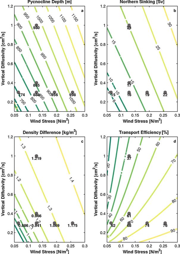
Fig. 3 Governing polynomials for each subcase of the model, where
the equilibrium state’s D is determined by the zero transitions of the
minimal Dq beyond which no physical solution exists.
graphs. The horizontal dotted line marks the zero, while the grey This feature is derived from the governing eq. (11) which
shaded area indicates negative D without physical relevance. The reduces to a fourth order polynomial in the mixing limit
polynomial of degree five (orange line) represents the entire model
with its standard parameters. Only two of its roots are positive and thus CN q0 bS S0 FN D4 þ CN q0 CU aT Dh D3 þ CU2 ¼ 0: ð13Þ
have a physical meaning. The smaller one at D = 613 m denotes the
stable state while the larger root, at D~ ¼ 1713 m, must be an unstable The functional form of the left hand side is depicted in
solution. The polynomial of degree three (blue line), representing the Fig. 3 (green dashed-dotted line) together with the general
wind-driven case, has also two relevant solutions D = 542 m and case. Using D ¼ CU =mN , eq. (13) can be rewritten in terms
D~ ¼ 1394 m. In addition, the mixing-driven case is depicted by the
of the volume transport
fourth order polynomial (green line). Only two real solutions are
detected, a stable one at D = 526 m and an unstable one at D~ ¼ 909 m m4N CN q0 CU2 aT jDhj mN þ CN q0 CU2 bS S0 FN ¼ 0: ð14Þ
any realistic situation, our analysis of the equation will be Both equations can be solved analytically. We omit the com-
restricted to Dh \ 0. plicated functional form here and rather provide expressions
The governing polynomial has five mathematical roots for conceptually interesting characteristics of the solution.
for D (see Fig. 3, orange line), each representing an equi- As shown in Fig. 4 no real positive solution for the
librium state of our model. Since negative or imaginary oceanic pycnocline exists for northern freshwater fluxes
pycnocline depths do not have an interpretation in our beyond a critical value F*M. This flux is defined by the zero
model set-up, only the positive roots are of interest. Among transition of the determinant (Fig. 4a, vertical light black
this physical solutions, some might be unstable under the line) which is defined by the polynomial in eq. (13). The
time-dependent dynamics of the model. We will not discriminant is presented in Appendix 2.1 and its root
explicitly compute the Lyapunov-exponents of the system, yields an equation for the critical freshwater flux
but let the numerical integration determine the stability. 2=3 4=3
3ð2CN q0 Þ1=3 CU aT
The parameter choice of Table 1 yields a stable state with a
FM ¼ jDhj4=3 : ð15Þ
8bS S0
pycnocline depth of D = 613 m (see Table 2). Since
adjacent solutions cannot share the same stability proper- In contrast to the Rahmstorf (1996) model which yields a
ties the other zero transition in Fig. 3 with D = 1,713 m quadratic dependence of the critical freshwater flux on the
represents an unstable solution. north–south temperature difference F ¼ ka2T Dh2 =ð4bS S0 Þ,
A more robust argument for the stability properties the pycnocline dynamics in our model reduce this
is obtained by the sign of the governing polynomial. sensitivity.2 The derivative qD/qFN is infinite at F*M for
For positive D (and as long as D\ðCW þ the stable physical solution (see Appendix 2.1 and Fig. 4a),
pffiffiffiffiffiffiffiffiffiffiffiffiffiffiffiffiffiffiffiffiffiffiffiffiffiffiffiffiffiffi
CW2 þ 4 C C Þ=ð2C Þ ¼ 2; 191 mÞ, the polynomial is
E U E
proportional to the time derivative of oD=ot. Thus an initial 1
Since the southern box is now disconnected from the other basins,
value of D = 0 m would increase because the polynomial is the corresponding salinity eq. (6) requires zero southern freshwater
positive. But when the first root is exceeded at D = 613 m, flux FS = 0 in order to obtain an equilibrium solution.Obviously this
the polynomial and thus oD=ot become negative and D does not affect the pycnocline depth D (cp. eq. 11), nor the volume
transports. It only has an impact on the various box salinities.
decreases. Consequently this root represents a stable steady 2
Here k is a positive constant which might depend on a prescribed
state. The corresponding solutions for the salinity equations pycnocline depth but not on Dh. In our model, k is quadratic in the
are separately presented in Appendix 4. pycnocline depth.
123J.J. Fürst, A. Levermann: Minimal overturning model 245
Fig. 4 Purely mixing-driven
case: dependence of the
equilibrium solution on the
northern freshwater input FN.
Grey shaded areas indicate
negative values either for D or
mN. The stable branch for the
pycnocline depth (a, black
heavy line) is in correspondence
with the solution in Fig. 3. The
unstable branch (a, dashed
black heavy line) shows a pole
with a change in sign at no
freshwater flux. This panel also
shows the real part of imaginary
solutions (a, dark grey lines) to
give an impression of the
distribution of the solutions.
Surpassing a certain freshwater
flux, no physically meaningful
solution can be obtained. This
point is marked by the change of
sign in the determinant (a-e,
black light line). In panel (b),
the behaviour of the northern
sinking (stable and unstable
branch) is depicted, clarifying
the abrupt change from one
regime to the other. The other
panels (c-f) give an overview of
the characteristics of the stable
solution. Remarkable are the
identity SN ¼ SD (b), the
existence of a minimal density
difference and the scaling of the
northern sinking with Dq1=3 (f)
which provides an additional equation to determine further circulation grows without bounds. The reasons are the iden-
properties of the critical point. tity mN ¼ mU ¼ CU =D in the mixing case and the fact that an
1=3 infinite freshwater flux causes the pycnocline depth to vanish.
4CU This is not the case for a purely wind-driven overturning.
DM ¼ ð16Þ
CN q0 aT jDhj
2 1=3 3.2 Wind-driven overturning
CU CN q0 aT
ðmN ÞM ¼ jDhj ð17Þ
4 Next, we consider the purely wind-driven case, CU = 0. In
Equations (12) and (17) give the critical density difference this limit, eq. (1) reduces to a quadratic equation in D and
provides a relation between the pycnocline depth and the
q 0 aT kg density difference. The only physical solution is
DqM ¼ jDhj ¼ 0:40 3 : ð18Þ
4 m sffiffiffiffiffiffiffiffiffiffiffiffiffiffiffiffiffiffiffiffiffiffiffiffiffiffiffiffiffi !
CE 4CN CW Dq
Despite the different scaling of F*M in Rahmstorf (1996), D¼ 1þ 1 :
2CN Dq CE2
the critical density difference scales linear with Dh in both
models. The decline of D with increasing Dh results in a Insertion into eq. (5) yields
weaker dependence of the critical northern sinking on Dh sffiffiffiffiffiffiffiffiffiffiffiffiffiffiffiffiffiffiffiffiffiffiffiffiffiffiffiffiffi !
compared to the linear dependence in Rahmstorf (1996). CE2 4CN CW Dq
A qualitative difference to the wind-driven case (Subsect. mN ¼ CW 1þ 1 : ð19Þ
2CN Dq CE2
3.2) emerges in the limit of highly negative northern fresh-
water fluxes. Dividing the governing eq. (13) by FN and The relation between mN and the density difference is
taking the limit FN ! 1 shows that the overturning very different from the mixing case. While no power law
123246 J.J. Fürst, A. Levermann: Minimal overturning model
exists for the entire range of Dq, the northern sinking 3.3 Full problem
approaches the (constant) strength of the southern ocean
upwelling, mW ¼ CW , for increasing density difference Dq. Though no complete analytic solution can be obtained for
On the other hand, for a vanishing density difference, the the full model (eq. (11)), some analytic insight can be
northern sinking tends to the unphysical limit mN ! 1 gained. A formal expansion of the steady state pycnocline
(see eq. (19)). The crucial question is if the variable Dq can dynamics with respect to the parameter set ðCE ; CU Þ
indeed become arbitrarily small in the wind-driven case. around the purely wind-driven case mN ¼ mW , i.e.
For this, set CU = 0 in the full governing eq. (11) to obtain ðCE ; CU Þ ¼ ð0; 0Þ, yields
the complete equilibrium dynamics. sffiffiffiffiffiffiffiffiffiffiffiffiffiffi sffiffiffiffiffiffiffiffiffiffiffiffiffiffi
ð1Þ CW CN Dq0
þ D3 CN q0 CE aT Dh mN ¼ CW CE þ CU ð23Þ
CN Dq0 CW
þ D2 CE2 þ CN q0 CW aT Dh þ CN q0 bS S0 FN ð20Þ
2
D 2CE CW þ CW ¼0 with
Using D ¼ ðCW mN Þ=CE we can transform this equation SO F N
Dq0 Dqjð0;0Þ ¼ q0 bS þ aT Dh ð24Þ
into an expression for the northern sinking CW
þ m3N CN q0 CW
2
bS S0 FN Each of the three terms in (23) can be understood in
2 2
þ mN CE 2CN q0 CW aT Dh þ CN q0 bS S0 FN light of the former limits of purely wind-driven and
ð21Þ mixing-driven circulations. The first term is the Southern
þ mN CN CW q0 ðCW aT Dh 2bS S0 FN Þ
Ocean upwelling, a constant contributor balancing the
þ CN CW q0 aT Dh ¼ 0:
northern sinking. It is reduced by the eddy return flow
Both equations for the wind-driven case show a third order represented by the second term. An additional contribution
polynomial which can be solved analytically. As in the emerges through the low-latitudinal upwelling of the third
mixing case a stable physical solution exists up to a critical term. This approximation holds reasonably well for the
threshold of the northern freshwater flux FN \ FW
(see parameter set of Table 1 for a realistic range of density
Fig. 5a–e, light vertical line). This critical freshwater flux differences (Fig. 7f, light line).
F*W is determined by the only real root of the correspondent For the full problem, an analytic treatment of the critical
discriminant which shows a third order in FN (cp. Appendix freshwater flux F*F is not possible since the discriminant !F
2.2). Since the analytic solution is complicated it is only (eq. (60)) is a fifth order polynomial in FN (cf. Appendix 2.3).
depicted in Fig. 5. As an alternative to analysing the full However, the intermediate value theorem states, that a fifth
solutions, we focus on the sensitivity of F*W on the North- order polynomial has at least one real root. For a physical
South temperature difference retrieved by the derivative of choice of parameters (positive CN ; CE ; CW ; CU ), the full
the discriminant with respect to Dh (see Appendix 2.2). This problem therefore always exhibits a critical freshwater flux
derivative can suitably be approximated for realistic F*F. This value can now be estimated by using the linearised
temperature differences from the limit Dh ! 1 model eq. (23). The discriminant of this second order poly-
oFW
oFW
aT C W nomial in D provides a second order polynomial to be solved
lim ¼ *
for FF(appr) . One of the two solutions is physically interesting
oDh Dh!1 oDh bS S0
2
ð22Þ and yields the approximated critical freshwater flux
CE
for jDhj ;
CN q0 CW aT CW Dq0
FFðapprÞ ¼ þ aT Dh ð25Þ
bS S0 q0
which is given as a slope in addition to the full dependence
0 1
in Fig. 6 (dashed blue line). This finding comprises that the pffiffiffiffiffiffiffiffiffiffiffiffiffiffiffiffiffiffiffiffiffiffiffiffiffiffiffiffiffiffi 2
2
function FW
ðDhÞ becomes quasi-linear for large tempera- BCW þ CW þ 4 CE CU C
Dq0 ¼ @ qffiffiffiffiffi A
ture differences. Figure 6 indicates that it also is a good 2 CCWN CU ð26Þ
approximation for realistic Dh. Moreover, it is shown that
kg
aT CW =ðbS S0 Þ jDhj is an upper constraint for the actual ¼ 0:29
critical freshwater flux F*W for realistic temperature dif- m3
ferences (see Appendix 2.2). This relation first of all confirms that linearity of the critical
In the present case, the limit FN ! 1 causes the freshwater flux in Dh is not merely restricted to the wind
pycnocline depth D and consequently the eddy return flow driven case, but also serves well to approximate the full
mE to vanish (see eq. (20)). Thus, in contrast to the mixing problem. In both cases we find the same proportionality
case where northern sinking diverges, here the northern constant. Moreover, this approximation also provides an
sinking approaches the constant southern upwelling mW. estimate for the offset of this linear relation. This offset is
123J.J. Fürst, A. Levermann: Minimal overturning model 247
Fig. 5 Dependence of the 1500 38
a b
Pycnocline Depth [m]
equilibrium solution for the
1000
wind-driven case on the northern
Salinity [psu]
freshwater input FN. Grey 500 36
shaded areas indicate negative
values either for the pycnocline 0 SN
or the northern sinking. The −500 34 S
stable branch for the pycnocline U
depth (a, black heavy line) is in −1000 S
S
correspondence with the solution −1500 32
in Fig. 3. The negative solutions −2 0 2 −2 0 2
for D are assumed to have no Freshwater Flux [Sv] Freshwater Flux [Sv]
physical relevance. Nevertheless
another positive unstable 28
c
Northern Sinking [Sv]
(a, dashed black heavy line) and 20 d
Density [kg/m ]
the real part of an imaginary 27
3
15
branch (a, dark grey line) are
depicted to give an impression of 10 26
the structure of the solutions.
5 25
Exceeding a specific freshwater
flux FN, no physical meaningful 0
solution can be found. This point 24
is marked by the change of sign −5
23
in the determinant (a-e, vertical −2 0 2 −2 0 2
black light line). In panel (c), the Freshwater Flux [Sv] Freshwater Flux [Sv]
behaviour of the northern sinking
Density Difference [kg/m ]
(stable and unstable branch) is
3
10 10
e
Northern Sinking [Sv]
depicted, clarifying the abrupt f
change from on regime to the 8 9
other. A solely wind-driven
overturning imposes an upper 6 8
bound on the northern sinking.
The other panels (b-f) give an 4 7
overview of the characteristics of
2 6
the stable solution and (f)
exhibits the existence of a
0 5
minimal density difference DqW −2 0 2 0 0.5 1 1.5
Freshwater Flux [Sv] Density Difference [kg/m3]
3
proportional to the critical Dq , which itself is in this first- full
order approximation independent of the meridional temper-
Critical Freshwater Flux [Sv]
wind
2.5
ature gradient and totally determined by the model parame- mixing
ters. Equation (25) captures the dependency of F*F on Dh stommel
2
reasonably (Fig. 6). Another interesting detail is that the
critical freshwater flux of the full problem F*F exceeds the 1.5
ones from the wind- and the mixing-driven cases. This gives
rise to a discussion for the freshwater sensitivity of the model. 1
0.5
4 Overturning sensitivity to freshwater
0
−30 −25 −20 −15 −10 −5 0
o
The derivative omN =oFN gives a mathematical measure for Temperature Difference [ C]
the sensitivity of the northern sinking mNto changes in the
Fig. 6 Critical freshwater flux F* as a function of the meridional
intensity of the northern freshwater flux FN. This derivative temperature difference Dh for the mixing-driven, wind-driven and full
can be determined forthe Stommel (1961) model and for all problem. In the wind-driven case the sensitivity on Dh can be
our subcasesbut not for the approach of Gnanadesikan conveniently approximated by the value of the derivative oFW =oDh at
(1999).FN is here implicitly included via the parameter Dq minus infinity (blue dashed). This slope is again retrieved by
approximating the full problem (blue dashed), but in addition the
and one would need an extra equation to linkthem. How- offset can be determined (eq. (25)). The Dh dependence of Stommels
ever,for the mixing- and wind-driven case as well as for the F* with a prescribed pycnocline depth (chosen according to Fig. 8) is
full problem, the derivative omN =oFN is a function with a quadratic and thus most pronounced
123248 J.J. Fürst, A. Levermann: Minimal overturning model
Fig. 7 Dependence of the 1500 38
a b
Pycnocline Depth [m]
equilibrium solution for the full
1000
problem on the northern
Salinity [psu]
freshwater input FN. Grey 500 36
shaded areas indicate negative
values either for the pycnocline 0
SN
or the northern sinking. The −500 34 SU
stable branch for the pycnocline
depth (a, black heavy line) is in −1000 SS
correspondence with the
−1500 32
solution in Fig. 3. The negative −2 0 2 −2 0 2
solutions for D is assumed to Freshwater Flux [Sv] Freshwater Flux [Sv]
have no physical relevance. To
give an impression of how the 28
c
Northern Sinking [Sv]
solutions are distributed in the 20 d
phase space, panel (a) also
Density [kg/m3]
15 27
shows a positive unstable
(dashed black heavy line) and 10 26
the real part of imaginary
5 25
branches (dark grey lines).
Surpassing a specific freshwater 0
flux FN, no physical meaningful 24
solution can be found. This −5
23
point is marked by the change of −2 0 2 −2 0 2
sign in the determinant (a, black Freshwater Flux [Sv] Freshwater Flux [Sv]
light line). In the middle left
Density Difference [kg/m3]
panel, the behaviour of the 10
northern sinking (stable and e f
Northern Sinking [Sv]
unstable branch) is depicted, 8 16
clarifying the abrupt change
from one regime to the other. 6
14
Beside the other characteristics
(b-e), the complete solution (f, 4
heavy line) shows a scaling 12
2
whose major shape can be
adequately described via a
0 10
Taylor expansion (f, light black −2 0 2 0 0.5 1 1.5
line) Freshwater Flux [Sv] Density Difference [kg/m3]
pole of order one in FN (see Appendix 3). In the Stommel
model, the derivative is obtained from eq. (8) showing a
pole of order 12. In order to determine which model has the
highest sensitivity to freshwater input in the North Atlantic,
it is necessary to align the positions of the respective poles.
e pycnocline depth DS is a parameter in the Stommel
(1961) model, we choose it such that the pole of the
Stommel model is at the same position as the pole of the
mixing-driven case (Fig. 8). This is motivated by the
resemblance of the circulation described in the Stommel
model and in our mixing-driven case. Both exhibit only
one mixing-driven circulation cell connecting the various
boxes. This approach (cf. Appendix 3) yields
1=3
pffiffiffi CU
DS ¼ 3 : ð27Þ Fig. 8 Sensitivity of northern sinking to changes in surface fresh-
2CN q0 aT Dh water flux: In the Stommel model (black line) the sensitivity of mN to
For our parameters, the right hand side has a value of 564.1 changes in freshwater flux FN is higher than in our model with
m. Choosing a smaller DS, shifts the pole of the Stommel varying pycnocline. Thus independent of the physical driving process,
the pycnocline stabilises the overturning circulation up to the critical
model F*S to a lower position than the one for the mixing- threshold where no solution exists. In addition, considering all the
driven case F*M. Studying the wind-driven case and the full subcases of our model, the mixing-driven case is most sensitive
123J.J. Fürst, A. Levermann: Minimal overturning model 249
Fig. 9 Solutions to the
governing eq. (11) as a function
of the Southern Ocean wind
stress and the vertical
diffusivity. Results from
CLIMBER-3a are superimposed
as • symbols. The panels depict
(a) the pycnocline depth, (b) the
Northern sinking mN, (c) the
meridional density gradient and
(d) the transport efficiency .
This quantity determines the
fraction of the Northern sinking
supplied by the Southern Ocean
ðmW mE Þ=mN
problem, we find that considering some additional constraints mN. It is possible to show (Appendix 3) that the Stommel
on the parameter space, their respective poles F*W and F*F are (1961) model exhibits a higher sensitivity compared to the
located at higher positions than that of the mixing-driven case mixing case (also see Fig. 8), as long as DS fulfills a slightly
F*M (cp. Fig. 6 and app. 9). In fact these new constraints more stringent constraint. Accounting for a small correc-
hardly restrict a physical parameter choice. For our set of tions term (see Appendix 3), the constraint of eu. (27)
parameters, the constraint for the wind-driven case reads lowers slightly for our parameters to DS 558:4 m: This
implicitly D 913 m which holds for the entire stable, reduces FS by merely 4:6 103 Sv. The new constraint is
physical solution branch (cp. Fig. 5). In the full problem, the therefore well approximated by the more intuitive one of eq.
implicit constraint includes an additional lower limit 351 m B (27). However, even if F*S slightly surpasses this constraint
D B 1,329 m, which is violated but only in the non-physical (same order of magnitude 10-3Sv), the sensitivity of the
case of a strong, inverse northern freshwater flux (cp. Fig. 7) Stommel (1961) model would exceed that of the mixing-
Given the found sequence FS FM
\ FW
and driven case below a freshwater input in a close vicinity of
FM \FF , we now focus on the freshwater sensitivity of F*M (Fig. 8 and Appendix 3). In order to mutually compare
123250 J.J. Fürst, A. Levermann: Minimal overturning model
the freshwater sensitivities of the different cases in our With this model a similar parameter scan was conducted
model, the implicit expressions of the derivatives omN =oFN and already presented in Gnanadesikan (1999). The general
are used. Appendix 3 reveals that some additional param- response is in agreement with our results. However the
eter constraints grant that the freshwater sensitivity of mN in ocean model shows higher variations in the pycnocline
the mixing-driven case is higher than that for the wind- depth and overturning. This confirms the choice for the
driven case and the full problem (also see Fig. 8). These central transport processes to be feasible and supports that
new constraints are again not violated by our parameter set. the dynamics of the AMOC is well described by variations
Thus, independent of the predominant driving mechanism, in both the pycnocline depth and the meridional density
the dynamics of the model pycnocline stabilises the Stom- gradient.
mel overturning up to the critical threshold. The model can
even bear a lower density difference (DqM ¼ 0:40 kg=m3
and DqF 0:29 kg=m3 ). In correspondence with the find- 6 Discussion and conclusion
ing that the wind-driven overturning is limited by CW, this
case shows the lowest freshwater sensitivity below a small In this study we address the question on whether and to
positive FN. what extent the stability properties of the AMOC depends
on its driving processes that are associated with the
upwelling branches of the overturning (Kuhlbrodt et al.
5 Comparison with comprehensive ocean model 2007). At the moment two mechanisms are under discus-
sion: upwelling in the low latitudes induced by turbulent
For a brief validation of the qualitative behaviour of our mixing across isopycnals and an ascent of water masses in
conceptual approach, experiments with a model of inter- the latitudinal band of the Drake Passage due to diverging
mediate complexity were carried out varying vertical dif- westerly winds. We present a conceptual model which
fusivity and SO wind forcing. All results are based on includes both processes in addition to the salt-advection
simulation with CLIMBER-3a, described by Montoya et al. feedback considered at the heart of an AMOC instability.
(2005). It includes modules describing the atmosphere, The strength of our model lies in the possibility of studying
land-surface scheme as well as sea-ice. The three-dimen- qualitative differences between a mixing- or a wind-driven
sional oceanic component (MOM-3) has a horizontal res- overturning.
olution of 3:75 3:75 and 24 non-uniformly spaced First and foremost, considering the conceptual model to
levels covering the vertical extent. be in steady state, an analytic description is found for the
The first set of steady state experiments investigates the wind- and for the mixing-driven case (see Sect. 3) In the
influence of vertical background diffusivity in the ocean, mixing-driven case, it reproduces the classical scaling of
analoguous to (Mignot et al. 2006). Three experiments the northern sinking with j2=3 Dq1=3 introduced by Bryan
with vertical diffusivity of 0.3, 0.4 to 1:0 104 m2 =s were (1987). Set by the SO winds, the purely wind-driven
conducted. The second set of experiments follows Schewe overturning imposes an upper bound for the northern
and Levermann (2010) and analyses the influence of the sinking. For an overturning circulation which is powered
zonal wind stress in the Drake Passage on the MOC. An by both driving mechanisms, a corresponding approxima-
amplification of the zonal wind field was applied in a lat- tion of the northern sinking is found. This scaling relation
itudinal band between 71.25S and 30S with factors of (see eq. 23) provides an instructive equation for the
a = 0.5, 1.0, 1.5 and 2. Both experiments are closely respective influences of the two driving mechanisms and
linked to one of the two upwelling mechanisms powering the SO eddy transport. This comprehensive case and the
the AMOC. The wind experiments directly affect the rate purely wind-driven one exhibit no simple power law for the
of Ekman pumping in the SO, while changes in j excert entire range of Dq.
control on the low-latitudinal upwelling. The values for One of the main results is the existence of a critical
D; Dq; mN and mW mE are determined as described in threshold beyond which no AMOC can be sustained, i.e. no
Levermann and Fürst (2010). physical solution exists in our model. The existence of an
For appropriate parameters, our conceptual model cap- off-states for a wind-driven overturning was already sug-
tures the qualitative response of CLIMBER-3a to changes gested by Johnson et al. (2007) in a similar but slightly
in the magnitude of the two driving mechanisms (Fig. 9). more comprehensive model than presented here. They
This is not trivial since CLIMBER-3a allows for many computed the off-state by setting the northern sinking to
more complex feedback mechanisms than the conceptual zero. It should however be noted that their model as well as
model. Since parameter sensitivity is strongly dependent on the one presented here are designed for a situation with a
the used model, an other ocean general circulation model functioning overturning. While it is possible to determine
(GFDL Modular Ocean Model, Version 3.0) is consulted. the point at which solutions cease to exists, it is not obvious
123J.J. Fürst, A. Levermann: Minimal overturning model 251
that these models can be used to compute the off-state in by Park (1999) but the sensitivity reduces further for an
any realistic way. In a G99 set-up an off-state requires that overturning with SO upwelling. Less freshwater sensitivity
SO upwelling is compensated by eddy return flow in the might indeed pose a problem for AMOC monitoring since
Southern Ocean. While it is clear that the tracer budget of the threshold is not easily detected by a significant, pre-
heat and salinity can be closed in this fashion, it is not ceding slow-down (cp. Figs. 4, 5 and 7). It should be noted
obvious whether the same holds for the momentum bal- that the model presented here was designed as a minimal
ance. For this, eddies would need to transport significant model that captures the salt-advection feedback in combi-
amount of momentum and it is questionable that such a nation with a representation of both AMOC driving
flow is well described by the diffusion equation of Gent mechanisms. Levermann and Fürst (2010) recently showed
and McWilliams (1990) with one constant coefficient. that in order to capture the behaviour of the coupled cli-
Our conceptual model makes it possible to explore the mate model CLIMBER-3a under global warming an
existence and the position of the critical freshwater additional dynamical equation for the geometry of iso-
threshold. The dependences of this critical freshwater flux pycnal out-cropping in the SO is necessary.
are crucially dependent on the involved transport processes
and can be expressed as a function of the meridional Acknowledgments JJF thank his colleagues Tore Hattermann,
Daria Schönemann and Jacob Schewe for fruitful discussions that
temperature difference. In our model the relevant density improved the quality of the presented work. This work also profited
and thus temperature differences are taken between low from the constructive suggestions of the reviewers whom the authors
and high latitudes. Due to polar amplification this tem- want to express their gratitude.
perature difference is likely to decrease under future
warming (e.g. Cai and Lu (2007)). We find that the sen-
sitivity of the critical freshwater flux to the meridional Appendix 1: Scaling of the northern sinking
temperature difference is reduced from a quadratic
dependence in a Stommel model (Rahmstorf 1996) to one This section briefly presents five different approaches to
of the power 4/3 in the mixing-driven case and to 1 when formulate scaling laws for the northern sinking. For each
SO wind forcing is included. Physically this means that the approach, a short derivation is given, which identifies the
dynamics of the pycnocline depth causes the overturning to main assumptions and discusses their validity. In this
be more robust under atmospheric temperature forcing. context, the difference between two vertical scales is
Concerning freshwater forcing, climate models of emphasised, the pycnocline depth D and the level of no
intermediate complexity show a large spread in sensitivity motion K. The first description from Robinson (1960), also
and hysteresis position (Rahmstorf et al. 2005). In our called the classical scaling, assumes the meridional over-
conceptual model, such differences can be associated with turning circulation to be in geostrophic balance. The ver-
the dominant driving mechanism. An overturning partially tical derivative of the momentum equation in the steady
or exclusively powered by SO winds is able to bear higher state yields
freshwater fluxes than a purely mixing-driven circulation
ov oq
(with parameters chosen from Table 1 one finds F*M = 0.23 f ¼ g ; ð28Þ
oz ox
Sv compared to F*F & 0.60 Sv). The sensitivity of the
overturning to changes in freshwater fluxes in the North when the hydrostatic equation is applied. Here v denotes
Atlantic below the critical threshold also depends on the the meridional velocity, q is the ocean density field and g is
main driving mechanism (Sect. 4) Setting the pycnocline the gravitational constant.
depth in the Stommel model to a certain value DS allows the Two scales, one for the meridional velocity field V and
sensitivity comparison to our model. This is done by setting one for the characterisitic depth K of the vertical profile of
the critical freshwater input of the Stommel (1961) model horizontal velocities, are introduced. The second is identi-
to the same position as the threshold of the mixing-driven fied with the level of no motion, where the mean meridional
case. Under this parameter constraint, the freshwater sen- velocities vanish. Additionally using a scale for the zonal
sitivity of the northern sinking is less pronounced in the density gradient Dx q occurring over a length scale Lx gives
mixing-driven case than in a Stommel model. Under further g Dx q K
parameter constraints, we were able to show that a mixing- V¼ : ð29Þ
f q0 Lx
driven overturning is more sensitive to freshwater pertur-
bations than an AMOC driven by SO winds. One can thus In order to transform the zonal density gradient into a
conclude that the pycnocline dynamics stabilises the meridional one Dy q, the zonal and meridional velocity
northern sinking under changes in the northern freshwater scales are linked. Albeit a radical generalisation, a constant
flux. For the mixing-driven case this was already proposed ratio V = Ccl U is assumed.
123252 J.J. Fürst, A. Levermann: Minimal overturning model
g Dy q K approach is drawn from the assumption that a meridional
V ¼ Ccl ð30Þ pressure gradient causes a frictional western boundary
f q0 Ly
current which limits the deep water formation in the Nordic
Since we seek an expression for the Atlantic Seas. In contrast to this, Johnson and Marshall (2002) base
overturning, an integration over the zonal extent Lm and their scaling of the northern sinking on an ocean model of
the vertical extent K of the flow is conducted. This gives reduced gravity. It is built up by a surface layer of depth h
the classical scaling for the northern sinking and an infinitely deep and motionless lower layer of fixed
g Dy q Lm 2 density. In this set-up, the level of no motion is implicitly
mN ¼ V K Lm ¼ Ccl K ; ð31Þ
f q0 Ly equal to the pycnocline depth. Assuming a geostrophic
flow in the interior of the surface ocean basin to provide the
which is proportional to the meridional density gradient, to water needed for the northern sinking mN, the meridional
the ratio between zonal and meridional length scales Lm =Ly velocity becomes
and to the square of the level of no motion K. The
theoretical basis for this estimate constrains its spatial g Dz q oh
v¼ ; ð35Þ
applicability to (1) the geostrophic assumption which is not f q0 ox
valid near continental boundaries and to (2) the ad-hoc where Dz q is the vertical density difference between the
transformation from zonal to meridional density gradients. two layers. Since the depth h is a function of x, a zonal
Gnanadesikan (1999) suggests that a western boundary integration from the western to the eastern boundary leads
current exerts control on the northern sinking. Neglecting to
the velocity component perpendicular to the boundary, a Zxe
relation between the meridional pressure gradient and the gDz q 2
mN ¼ hvdx ¼ hE h2W ð36Þ
meridional velocity is derived 2f q0
xw
1 op o2 v gDz q ~2
¼ mr2 v ¼ m 2 ; ð32Þ ¼ D ; ð37Þ
q0 oy ox 2f q0
where r2 is the Laplacian and m is the dynamic viscosity in where hE ; hW are the layer depth at the eastern and western
the boundary current. For the second equality it is assumed boundary, respectively. The third step implies Johnson’s
that the zonal change in meridional velocity exceeds the
redefinition of the pycnocline depth D~ (Johnson et al.
changes in vertical and meridional direction by several
2007).
orders of magnitude (Montoya et al. 2005).
The main difference to previous scalings is a depen-
A scale analysis analogue to the previous paragraph
dence on a density gradient Dz q in the vertical direction. In
provides
addition this approach sees the reason for the geostrophic
V 1 Dy p Dy q D flow in a zonal tilt of the pycnocline depth. However, it is
m 2
¼ CG99 ¼ CG99 g ; ð33Þ
Lm q0 Ly q0 Ly argued that an outcropping of the pycnocline occurs at the
western boundary, while at the eastern boundary the py-
where the constant CG99 accounts for any effects of
cnocline is equal to D (Johnson et al. 2007). A funda-
geometry and boundary layer structure. For the second
mentally different approach is provided by Guan and
equality, where the hydrostatic equation is employed, a
Huang (2008) who introduce an energy constraint, instead
new vertical scale height D is introduced. This height
of the well known buoyancy constraint. The idea is that the
represents the density stratification of the ocean and is
energy supply is used for diapycnal mixing, which is
referred to as the pycnocline depth D.
described by a vertical advection-diffusion balance. Using
Integration yields another scaling law for the northern
a scale for the vertical density difference Dz q, the scale of
sinking
its vertical change Dz ðDz qÞ and another for the pycnocline
gL2m Dy q Lm depth D, the equation can be rewritten for a constant dia-
mN ¼ V K Lm ¼ CG99 DK: ð34Þ
m q0 Ly pycnal diffusivity j
j
In analogy with the classical scaling law, we again find wDz q ¼ Dz ðDz qÞ: ð38Þ
proportionality to a meridional density difference. D
However the relation between the Coriolis frequency f is Assuming an exponential density profile, the proportion-
replaced by the inverse of the zonal viscosity time scale in ality Dz ðDz qÞ Dz q becomes valid.
the western boundary current L2m/m. Another even more The gravitational potential energy (GPE) in a two-layer
important change is the proportionality to the product of box model, with a vertical density difference Dz q, increases
the pycnocline depth D and the level of no motion K. This due to vertical mixing with a rate of gjDz q (per unit
123You can also read