How Robust Standard Errors Expose Methodological Problems They Do Not Fix, and What to Do About It
←
→
Page content transcription
If your browser does not render page correctly, please read the page content below
Advance Access publication October 31, 2014                                             Political Analysis (2015) 23:159–179
                                                                                                   doi:10.1093/pan/mpu015

          How Robust Standard Errors Expose Methodological
         Problems They Do Not Fix, and What to Do About It

                                                   Gary King
                       Institute for Quantitative Social Science, 1737 Cambridge Street,
                                   Harvard University, Cambridge, MA 02138
                                e-mail: king@harvard.edu (corresponding author)

                                             Margaret E. Roberts
                          Department of Political Science, 9500 Gilman Drive, #0521,
                           University of California San Diego, La Jolla, CA 92093

                                                                                                                               Downloaded from http://pan.oxfordjournals.org/ at Harvard Library on May 25, 2015
                                      e-mail: molly.e.roberts@gmail.com

                                             Edited by Janet Box-Steffensmeier

       “Robust standard errors” are used in a vast array of scholarship to correct standard errors for model
       misspecification. However, when misspecification is bad enough to make classical and robust standard
       errors diverge, assuming that it is nevertheless not so bad as to bias everything else requires considerable
       optimism. And even if the optimism is warranted, settling for a misspecified model, with or without robust
       standard errors, will still bias estimators of all but a few quantities of interest. The resulting cavernous gap
       between theory and practice suggests that considerable gains in applied statistics may be possible. We seek to
       help researchers realize these gains via a more productive way to understand and use robust standard errors; a
       new general and easier-to-use “generalized information matrix test” statistic that can formally assess
       misspecification (based on differences between robust and classical variance estimates); and practical illustra-
       tions via simulations and real examples from published research. How robust standard errors are used needs to
       change, but instead of jettisoning this popular tool we show how to use it to provide effective clues about model
       misspecification, likely biases, and a guide to considerably more reliable, and defensible, inferences.
       Accompanying this article is software that implements the methods we describe.

1    Introduction
The various “robust” techniques for estimating standard errors under model misspecification are
extremely widely used. Among all articles between 2009 and 2012 that used some type of regression
analysis published in the American Political Science Review, 66% reported robust standard errors.
In International Organization, the figure is 73%, and in American Journal of Political Science, it is
45%. Across all academic fields, Google Scholar finds 75,500 articles using “robust standard
errors,” and about 1000 more each month.1
   The extremely widespread, automatic, and even sometimes unthinking use of robust standard
errors accomplishes almost exactly the opposite of its intended goal. In fact, robust and classical
standard errors that differ need to be seen as bright red flags that signal compelling evidence of
uncorrected model misspecification. They highlight statistical analyses begging to be replicated,
respecified, and reanalyzed, and conclusions that may need serious revision.
   Robust standard errors have a crucial role in statistical theory in a world where models are
almost never exactly right. They can be used in practice to fix a specific part of model estimation,

Authors’ Note: Our thanks to Neal Beck, Tim Büthe, Andrew Hall, Helen Milner, Eric Neumayer, Rich Nielsen, Brandon
Stewart, and Megan Westrum for many helpful comments, and David Zhang for expert research assistance. All data and
information necessary to replicate our work are available in a Dataverse replication file at King and Roberts (2014).
 1
   We conducted the search on 7/28/14 with the term “robust standard errors” (with the quotation marks). This figure is
   an underestimate since it does not count other names such as White, Huber-White, Eicker, Eicker-White, clustered,
   cluster-robust, panel-corrected, sandwich, heteroskedasticity-consistent, autocorrelation-consistent, etc.

ß The Author 2014. Published by Oxford University Press on behalf of the Society for Political Methodology.
All rights reserved. For Permissions, please email: journals.permissions@oup.com

                                                             159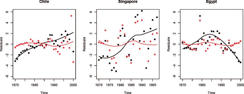
160                                          Gary King and Margaret E. Roberts

when special circumstances hold. However, they are often used in applications as a default setting,
without justification (sometimes even as an effort to inoculate oneself from criticism), and without
regard to the serious consequences their use implies about the likely misspecification in the rest of
one’s model. Moreover, a model for which robust and classical standard error estimates differ is
direct confirmation of misspecification that extends beyond what the procedure corrects, which
means that some estimates drawn from it will be biased—often in a way that can be fixed but not
merely by using robust standard errors. Drawing valid substantive claims from a model that
evidence in the data conclusively demonstrates is at least partly misspecified is possible in
specialized circumstances, but only with considerable justification.
    The problem at hand is not merely a lost opportunity to slightly improve inferences. And this is
not an example of the literature failing to live up to the high standards of abstract statistical theory
(or the methodological intelligentsia), or where fixing the problem would only occasionally make a
practical difference. Instead, it appears that a large fraction of the articles published across fields is
based on models that have levels of misspecification that are detectable even in their own data and
without new assumptions. For every one of these articles, at least some quantity that could be

                                                                                                                                Downloaded from http://pan.oxfordjournals.org/ at Harvard Library on May 25, 2015
estimated is biased. Exactly how important the biases are in any one article from a substantive point
of view is an open question, but scholarly articles should be based on evidence rather than
optimism.
    Consider a simple and well-known example, in the best case for robust standard errors:
The maximum likelihood estimator of the coefficients in an assumed homoskedastic linear-
normal regression model can be consistent and unbiased (albeit inefficient) even if the data-gener-
ation process is actually heteroskedastic. And although classical standard errors will be biased in
this circumstance, robust standard errors are consistent so long as the other modeling assumptions
are correct (i.e., even if the stochastic component and its variance function are wrong).2
    Thus, the promise of this technique is substantial. However, along with the benefits come some
substantial costs. Consider two situations. First, even if the functional form, independence, and
other specification assumptions of this regression are correct, only certain quantities of interest
can be consistently estimated. For example, if the dependent variable is the Democratic proportion
of the two-party vote, we can consistently estimate a regression coefficient, but not the probability
that the Democrat wins, the variation in vote outcome, risk ratios, vote predictions with confidence
intervals, or other quantities. In general, computing quantities of interest from a model, such as by
simulation, requires not only valid point estimates and a variance matrix, but also the veracity
of the model’s complete stochastic component (King, Tomz, and Wittenberg 2000; Imai, King, and
Lau 2008).
    Second, if robust and classical standard errors diverge—which means the author acknowledges
that one part of his or her model is wrong—then why should readers believe that all the other parts
of the model that have not been examined are correctly specified? We normally prefer theories
that come with measures of many validated observable implications; when one is shown to be
inconsistent with the evidence, the validity of the whole theory is normally given more scrutiny,
if not rejected (King, Keohane, and Verba 1994). Statistical modeling works the same way: each of
the standard diagnostic tests evaluates an observable implication of the statistical model. The more
these observable implications are evaluated, the better, since each one makes the theory vulnerable
to being proven wrong. This is how science progresses. According to the contrary philosophy of
science implied by the most common use of robust standard errors, if it looks like a duck and smells
like a duck, it is just possible that it could be a beautiful blue-crested falcon.
    Fortunately, a simple, easy-to-understand, and more powerful alternative approach to marshal-
ing robust standard errors for real applications is nevertheless available: If your robust and classical
standard errors differ, follow venerable best practices by using well-known model diagnostics

2
    The term “consistent standard errors” is technically a misnomer because as N ! 1, the variance converges to zero.
    However, we follow
                   pffiffiffiffi standard practice in the technical literature by defining a variance estimator to be consistent when
    the variance of Nð^  Þ rather than ^ is statistically consistent.
The Problem with Robust Standard Errors                                          161

to evaluate and then to respecify your statistical model. If these procedures are successful, so that
the model now fits the data and all available observable implications of the model specification are
consistent with the facts, then classical and robust standard error estimates will be approximately
the same. If a subsequent comparison indicates that they differ, then revisit the diagnostics, respe-
cify the model, and try again. Following this advice is straightforward, consistent with long-
standing methodological recommendations, and, as we illustrate in real examples from published
work, can dramatically change substantive conclusions. It also makes good use of the appropriate
theory and practice of robust standard errors.
    To be clear, we are not recommending that scholars stop using robust standard errors and switch
to classical standard errors. Nor do we offer a set of rules by which one can choose when to present
each type of uncertainty estimate. Instead, our recommendation—consistent with best practices in
the methodological literature—is to conduct appropriate diagnostic procedures and specify one’s
model so that the choice between the two becomes irrelevant.3
    In applied research, the primary difficulty following the advice the methodological community
recommends is understanding when the difference between classical and robust standard errors is

                                                                                                                                    Downloaded from http://pan.oxfordjournals.org/ at Harvard Library on May 25, 2015
large enough to be worth doing something about. The purpose of this article is to offer the expos-
ition, intuition, tests, and procedures that can span the divide between theory and applied work.
We begin with a definition of robust standard errors in Section 2 and a summary of their costs and
benefits in Section 3. We then introduce existing formal tests of misspecification, including our
extensions and generations in Section 4. Then, for three important published analyses with appli-
cations using robust standard errors, we show how our proposed procedures and tests can reveal
problems, how to respecify a model to bring robust and classical standard errors more in line (thus
reducing misspecification), how confidence in the new analysis can increase, and how substantive
conclusions can sometimes drastically change. To provide intuition, we introduce the concepts
underlying the examples first via simulated data sets in Section 5 and then via replications of the
original data from the published articles in Section 6. Section 7 concludes.

2      What Are Robust Standard Errors?
We first define robust standard errors in the context of a linear-normal regression model with
possible misspecification in the variance function or conditional expectation. The analytical expres-
sions possible in this simple case offer considerable intuition. We extend these basic ideas to any
maximum likelihood model and then to more complicated forms of misspecification.

2.1      Linear Models
We begin with a simple linear-normal regression model. Let Y denote an n  1 vector of random
variables and X a fixed n  k matrix, each column of which is an explanatory variable (the first
usually being a column of ones). Then the stochastic component of the model is normal with n  1
mean vector  and n  n positive definite variance matrix VðYjXÞ  : Y  Nð; Þ. Throughout,
we denote the systematic component as EðYjXÞ   ¼ X, for k  1 vector of effect parameters .

3
    Our work only applies to model-based inference which, although the dominant practice, is not the only theory of
    inference. Indeed, some researchers forgo models and narrow their inferences to certain quantities that, under Fisher
    (1935), Neyman (1923), or other theories, can be estimated without requiring the assumptions of a fully specified model
    (e.g., a sample mean gives an unbiased estimate of a population mean without a distributional assumption). In these
    approaches without a model, classical standard errors are not defined, and the correct variance of the non-model-based
    estimator coincides with the robust variance. For these approaches, our recommended comparison between robust and
    classical standard errors does not apply. The popularity of model-based inference may stem from the fact that models
    are often the easiest (or the only) practical way to generate valid estimators of some quantities. Likelihood or Bayesian
    theories of inference can be applied to an extremely wide range of inferences and offer a simple, standard approach to
    creating estimators (King 1989a). The alternative approach that led to robust standard errors begins with models but
    allows for valid inference under certain very specific types of misspecification and for only some quantities of interest. It
    explicitly gives up the ability to compute most quantities from the model in return for the possibility of valid inference
    for some (Eicker 1963; Huber 1967; White 1996).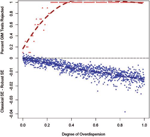
162                                 Gary King and Margaret E. Roberts

For this exposition, we focus on the variance matrix which, thus far, has considerable flexibility:
                                       0 2                       1
                                           11  212 . . .  21n
                                       B 2                       C
                                       B  21  222 . . .  22n C
                                       B                         C
                                  ¼B  B             ..
                                                                 C:
                                                                 C                              ð1Þ
                                       B :      :        . : A   C
                                       @
                                             2n1    2n2   . . .  2nn
If we rule out autocorrelation by assuming independence between Yi and Yj for all i 6¼ j after
conditioning on X, then we specialize the variance matrix to
                                       0 2                   1
                                          11 0      ... 0
                                       B                     C
                                       B 0  222 . . . 0 C
                                       B                     C
                                1 ¼ B B            .
                                                             C:
                                                             C                             ð2Þ
                                       B :      :     ..   : C
                                       @                     A

                                                                                                           Downloaded from http://pan.oxfordjournals.org/ at Harvard Library on May 25, 2015
                                             0       0       . . .  2nn

     Finally, if we also assume homoskedasticity, we are left with the classical linear-normal regres-
sion model (Goldberger 1991). To do this, we set the variance matrix to VðYjXÞ ¼  2 I, where  2 is a
scalar and I is an n  n identity matrix. That is, we restrict equation (2) to  ¼  2 I or
 211 ¼  222 ¼ . . . ¼  2nn . (With this restriction, we could rewrite the entire model in the simpler
scalar form as Yi  NðXi ;  2 Þ along with an independence [no autocorrelation] assumption.)

2.2   Estimators
Let y be an n  1 observed outcome variable, a realization of Y from the model with VðYjXÞ ¼  2 I.
Then the maximum likelihood estimator (MLE) for  is the familiar least squares solution b ¼ Ay,
where A ¼ Q1 X0 , Q ¼ X0 X, with variance VðbÞ ¼ VðAyÞ ¼ AVðyÞA0 ¼ A 2 IA0 ¼  2 Q1 . It is also
well known that the MLE is normal in repeated samples. Thus, bjX  Nð;  2 Q1 Þ.
   We can estimate  2 with its MLE ^ 2 ¼ e0 e=n (or small sample approximation) and
where e ¼ y  Xb is an n  1 vector of residuals. The classical standard errors are the square
root of the diagonal elements of the estimate of V(b).
   For illustration, consider estimates of two quantities of interest that may be estimated from this
model. First is , which under certain circumstances could include a causal effect. For the second,
suppose the outcome variable is the Democratic proportion of the two-party vote, and we are
interested in, for given values of X which we denote x, the probability that the Democrat wins:
Pr ðY > 0:5jX ¼ xÞ. This is straightforward to calculate analytically under this simple model, but
for intuition in the more general case, consider how we compute this quantity by simulation. First,
simulate estimation uncertainty by drawing  and  2 from their distributions (or in the more
general case, for simplicity, from their asymptotic normal approximations), insert the simulated
values, which we denote by adding tildes, into the stochastic component, NðX; ~ ~ 2 IÞ, and finally add
fundamental uncertainty by drawing Y~ from it. Then, to compute our estimate
of Pr ðY > 0:5jX ¼ xÞ by simulation, repeat this procedure a large number of times and count
the proportion of times we observe Y~ > 0:5. A key point is that completing this procedure
requires all parts of the full model.

2.3   Variance Function Misspecification
Suppose now a researcher uses the classical linear-normal regression model estimation procedure
assuming homoskedasticity, but with data generated from the heteroskedastic model, that is, with
VðYjXÞ ¼ 1 from equation (2). In this situation, b is an unbiased estimator of . If the heteroske-
dasticity is a function of X, then b is still unbiased but inefficient and with a classical variance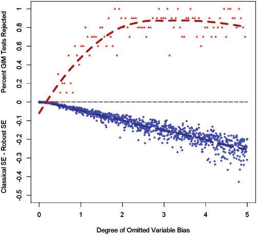
The Problem with Robust Standard Errors                                        163

estimator that is inconsistent because VðbÞ ¼ VðAyÞ ¼ AVðyÞA0 ¼ A1 A0 6¼  2 Q1 . As importantly,
and regardless of whether the heteroskedasticity is a function of X, other quantities of interest from
the same model such as Pr ðY > 0:5jX ¼ xÞ can be very seriously biased. This last fact is not widely
discussed in regression textbooks but can be crucial in applications.
   Robust standard errors of course only try to fix the standard error inconsistency. Fixing this
inconsistency seems difficult because, although A is known,  under equation (2) has n elements
and so it was long thought that consistent estimation would be impossible. In other words, for an
estimator to be consistent (i.e., for the sampling distribution of an estimator to collapse to a spike
over the truth as n grows), more information must be included in the estimator as n increases, but if
the number of quantities to be estimated increases as fast as the sample size, the distribution never
collapses.
   The solution to the inconsistency problem is technical, but we can give an intuitive explanation.
First define a k  k matrix G ¼ X0 1 X and then rewrite the variance as VðbÞ ¼ A1 A0 ¼ Q1 GQ1
(the symmetric mathematical form of which accounts for its “sandwich estimator” nickname).
Interestingly, even though 1 has n unknown elements, and so increases with the sample size, G

                                                                                                                                 Downloaded from http://pan.oxfordjournals.org/ at Harvard Library on May 25, 2015
remains a k  k matrix as n grows. Thus, we can replace  2i with its inconsistent but unbiased
estimator, e2i , and we have a new consistent estimator for the variance of b under either type of
misspecification (White 1980, 820).
   Crucially for our purposes, this same result provides a convenient test for heteroskedasticity:
Run least squares, compare the robust and classical standard errors, and see if they differ. Our
preference is for this type of direct comparison, since standard errors are on the scale of the
quantity being estimated and so the extent of differences can be judged substantively.4 However,
researchers may also wish to use formal tests that compare the entire classical and robust variance
matrices, as we discuss in more detail below (Breusch and Pagan 1979; White 1980; Koenker 1981;
Koenker and Bassett 1982).

2.4      Other Types of Misspecification
We now go another step and allow for an incorrect variance function, conditional expectation
function, or distributional assumption. In this general situation, instead of using b to estimate  in
the true conditional expectation function EðYjXÞ ¼ X, we treat this function as unknown and
define our estimand to be the “best linear predictor”—the best linear approximation to the true
conditional expectation function (see Goldberger 1991; Huber 1967). In any or all of these types of
misspecification, b still exists and has a variance, but differs from the classical variance for the same
reason as above: VðbÞ ¼ VðAyÞ ¼ AVðyÞA0 ¼ A1 A0 6¼  2 Q1 , resulting in the classical standard
errors being inconsistent. So long as no autocorrelation is induced, we can still use the same
estimator as in Section 2.3 to produce a consistent estimate of V(b). (For intuition as to why an
incorrect functional form can sometimes show up as heteroskedasticity, consider what an omitted
variable can do to the residuals: unexplained variation goes into the variance term, which need not
have a constant effect.)
   Numerous generalizations of robust standard errors have been proposed for many different
types of misspecification, and for which the intuition offered above still applies. Versions of
robust standard errors have been designed for data that are collected in clusters (Arellano 1987),
with serial correlation (Bertrand, Duflo, and Mullainathan 2004), from time-series cross-sectional
(or panel) data (Beck and Katz 1995), via time-series cross-sections with fixed effects and inter-
temporal correlation (Kiefer 1980), with both heteroskedasticity and autocorrelation (Newey and

4
    Judging whether the difference between robust and classical standard errors is substantially meaningful is not related to
    whether using one versus the other changes the “significance” of the coefficient of interest; indeed, this significance is
    not even necessarily related to whether there exists a statistically significant difference between classical and robust
    standard errors. Instead, researchers should focus on how much the uncertainty estimate (standard error, implied
    confidence interval, etc.) is changing relative to the metric implied by the parameter or other quantity of interest
    being estimated; usually this is directly related to the metric in which the outcome variable is measured and so
    should be meaningful. We also offer a more formal test below.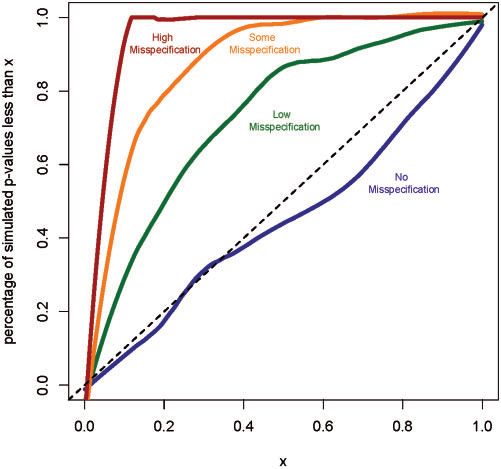
164                                          Gary King and Margaret E. Roberts

West 1987), with spatial correlation (Driscoll and Kraay 1998), or which estimate sample rather
than population variance quantities (Abadie, Imbens, and Zheng 2011). These different versions
of robust standard errors optimize variance estimation for the special cases to which they apply.
They are also useful for exposing the particular types of misspecification that may be present
(Petersen 2009).

2.5      General Maximum Likelihood Models
We now generalize the calculations above designed for the linear-normal case to any linear or
nonlinear maximum likelihood model. If fðyi jÞ is a density describing the data-generating
process for Q an observation, and we assume independencePacross observations, then the likelihood
function is ni¼1 fðYi jÞ and the log-likelihood is LðÞ ¼ ni¼1 log fðYi jÞ.
   The generalization of the White estimator requires the first and second derivatives of the
log-likelihood. The bread of the sandwich estimator, P, is now the Hessian
               P       2
P ¼ L ðÞ ¼ ni¼1   logfðy
       00
                              i jÞ
                                    . The meat of the sandwich, M, is the square of the gradient

                                                                                                                               Downloaded from http://pan.oxfordjournals.org/ at Harvard Library on May 25, 2015
                           2
                           j
                   P     h             iT h          i
M ¼ cov½L ðÞ ¼ ni¼1  logfðyi jÞ  logfðyi jÞ . We then write the robust variance matrix as
            0

                                      j             j

VðbÞ ¼ P1 MP1 . All other results apply directly.5

3      Costs and Benefits of Robust Estimation under Misspecification
3.1      Uses
Models are sometimes useful but almost never exactly correct, and so working out the theoretical
implications for when our estimators still apply is fundamental to the massive multidisciplinary
project of statistical model building. In applications where using a fully specified model leads to
unacceptable levels of model dependence and the assumptions necessary for robust standard errors
to work do apply, they can be of considerable value (Bertrand, Duflo, and Mullainathan 2004).
   However, the more common situation for applied researchers is importantly different. If we are
aware that a model is misspecified in one of the ways for which researchers have developed an
appropriate robust standard error, then in most situations the researcher should use that informa-
tion to try to improve the statistical model (Leamer 2010). Only in rare situations does it make
sense to prefer a misspecified model, and so if information exists to improve the chosen model, we
should take advantage of it. If insufficient time is available, then robust standard errors may be
useful as a shortcut to some information, albeit under greater (model misspecification) uncertainty
than necessary.
   Consider first the best-case scenario where the model is misspecified enough to make robust and
classical standard errors diverge but not so much as to bias the point estimates. Suppose also that
we can somehow make the case to our readers that we are in this Goldilocks region so that they
should then trust the estimates that can be made. In this situation, the point estimator is inefficient.
In many situations, inefficiency will be bad enough that improving the model by changing the
variance function will be preferable (Moulton 1986; Green and Vavreck 2008; Arceneaux and
Nickerson 2009). Because our point estimator is asymptotically normal, we can estimate  or
any deterministic function of it. This is sometimes useful, such as when a linear regression coeffi-
cient coincides with a causal effect, or when a nonlinear regression coefficient is transformed into
the expected value of the outcome variable.
   However, because the full stochastic component of the model is ignored by this technique, any
quantity based on the predictive distribution of the outcome variable cannot be validly estimated.
For example, we would not be able to obtain unbiased or consistent estimates of the probability
that the Democrat will win, confidence intervals on vote forecasts or counterfactual predictions,

5
    Note that the decomposition of the sandwich is slightly different in the general formulation than in the linear one
    described above. In the linear case, the bread is Q ¼ X0 X, whereas in the general formulation the bread is the Hessian.
    Of course, the linear case could be written in this formulation as well.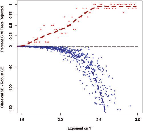
The Problem with Robust Standard Errors                           165

or most other related quantities. Since predictive distributions of the values of the outcome variable
are not available, we cannot use most of the usual diagnostic procedures, such as posterior
predictive checks, to validate that we are indeed in the Goldilocks region or otherwise provide
evidence that our modeling strategy is appropriate.
   To be more precise, consider a linear-normal regression model specification where robust and
classical standard errors differ, meaning that the model is misspecified. Suppose that we are in the
best-case scenerio where ^ is unbiased, and the robust estimator of the variance matrix is consistent.
Now suppose we need to simulate from the model, as in King, Tomz, and Wittenberg (2000),
in order to calculate some quantity of interest based on the outcome, such as the probability
that the Democrat wins. To do this, we need (1) random draws of the parameters from their
sampling distribution reflecting estimation uncertainty (e.g., ~  Nðy;        ^ Vð ^
                                                                                  ^ yÞÞ, which is no
problem), and (2) random draws of the outcome variable from the model. If the model was
correct, this second step would be
                                           Y~  NðX;
                                                   ~ ~ 2 Þ;                                        ð3Þ

                                                                                                          Downloaded from http://pan.oxfordjournals.org/ at Harvard Library on May 25, 2015
where ; ~ ~ 2 , and Y~ denote simulated values. However, although step (1) still works under
misspecification, step (2) and equation (3) do not apply. For a simple example of this, suppose X
is univariate and dichtomous and  2 is 1 for X ¼ 0 and 100 for X ¼ 1, or  2i ¼ 100  Xi . Clearly
in this case, it would make little sense to draw Y from a distribution with any one value of  2 .
If we were computing R1        the probability that the Democrat wins, we would need
Pr ðY > 0:5jXÞ ¼ 0:5 NðyjX; ~ 100  XÞdy. Even if for some reason we could believe that the nor-
mality assumption still applies under misspecification, using any fixed value of  2 to approximate
100  Xi would be a disaster for the substantive purpose at hand since it would yield the wrong value
of the probability for some or all observations.
   Under standard model diagnostic checking procedures, empirical tests are available for ques-
tions like these; when using robust standard errors, we have the advantage of not having to specify
the entire model, but we are left having to defend unverifiable theoretical assumptions. To be sure,
these assumptions are sometimes appropriate, although they are difficult to verify and so must be
considered a last resort, not a first line of defense against reviewers.
   In general, if the robust and classical standard errors differ, the cause could be misspecification
of the conditional expectation function, such as omitted-variable bias that would invalidate all
relevant point estimates, or it could be due to fundamental heteroskedasticity that will make
some point estimates inefficient but not biased, and others biased. One reaction some have in
this situation is to conclude that learning almost anything with or without robust standard
errors is hopeless (Freedman 2006). We suggest instead that researchers take the long-standing
advice in most textbooks and conduct appropriate diagnostic tests, respecify the model, and try to
fix the problem (Leamer 2010). For example, some authors have avoided misspecification by
modeling dependence structures, and ensuring that their fully specified models have observable
implications consistent with their data (Hoff and Ward 2004; Gartzke and Gleditsch 2008). But
however one proceeds, the divergence of the two types of standard errors is an easy-to-calculate
clue about the veracity of one’s entire inferential procedure, and so it should not be skipped,
assumed away, or used without comparison to classical standard errors.

4   A Generalized Information Matrix Test
We offer here a more formal test with clear decision rules for the difference between robust
and classical standard errors. To compute this test, we need a statistic and corresponding
null distribution to describe the difference between the robust and classical variance matrices.
This indeed is the foundation for the information matrix test proposed by White (1980) for
the linear case, and extended in diverse ways with different tests to other parametric models
by others (Breusch and Pagan 1979; Koenker 1981; Koenker and Bassett 1982). Instead of differ-
ent tests for each model, in this section, we develop a single “generalized information matrix”
(GIM) test that applies across all types of specific models and works much better in small, finite
samples.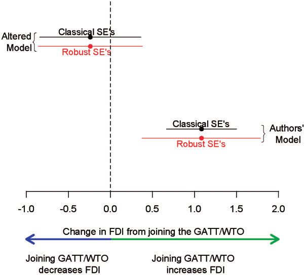
166                                     Gary King and Margaret E. Roberts

   To begin, note that the downside of the original information matrix test is that its asymptotic
distribution poorly approximates its finite sample distribution (Taylor 1987; Orme 1990; Chesher
and Spady 1991; Davidson and MacKinnon 1992). Since the statistic is based on two high-
dimensional variance matrices, a very large sample size is usually necessary for the asymptotics
to provide a reasonable approximation. Moreover, although this test can technically be applied to
any parametric model, the efficient form of the test is different for each individual model, resulting
in complexity for the user (Lancaster 1984; Orme 1988). As a result, general code for a diverse
array of models is not straightforward to create and does not presently exist in a unified form
in any commonly used software.
   The literature thus offers well-developed theory but nevertheless a difficult path for applied
researchers. Our GIM test is designed to meet the needs of applied statistics as a single, simple,
and formal measure of the difference between robust and classical standard errors that is easy to
apply, does not rely on asymptotics, and works for any parametric model.
   We first follow Dhaene and Hoorelbeke (2004) by using a parametric bootstrap for the variance
matrix of the test statistic (see Section 4.1). This allows for better small-sample performance, and

                                                                                                                    Downloaded from http://pan.oxfordjournals.org/ at Harvard Library on May 25, 2015
easy adaptability to any parametric model. Then, unlike previous approaches, we extend this
approach to clustered and time-series data, which are prevalent in many fields. This allows users
to compare and test for classical versus cluster or time-series robust variance matrices (see Section
4.2). This extension makes it possible for us to write easy-to-use, open-source R code that imple-
ments this test, and which we make available as a companion to this article. Below we also offer
Monte Carlo validation of the GIM test (Section 4.3) and discuss its limitations (Section 4.4).

4.1   An Introduction to Information Matrix Tests
For any maximum likelihood model, the classic variance matrix is the negative inverse of the
Hessian matrix, VC ðbÞ ¼ P1 . Since the robust variance matrix is defined as VR ðbÞ ¼ P1 MP1 ,
where M is the square of the gradient, we have VC ðbÞ ¼ VR ðbÞ when M ¼ P. A test of model
misspecification then comes by evaluating EðM þ PÞ ¼ 0, which is true under            P the model.
   To derive the test statistic, first, for observations y1 . . .yn , let D^ ij ¼ p1ffiffin nt¼1 ðM
                                                                                             ^ ij þ P^ ij Þ. Then
                                                                                 1
stack components of the matrix into a vector d.   ^ And finally, o ¼ d^0 V^ d^ is asymptotically 2
                                                                                                               q
distributed, where q is the length of d; ^ V^ is an asymptotic variance matrix, with a form derived
by White (1980), but many modifications of it have been proposed in the literature for different
assumptions and models.
   We derive the GIM test by estimating V with a parametric bootstrap, as in Dhaene and
Hoorelbeke (2004). To do this, we first estimate the MLE ^ and test statistic d^ for the data
and the model we are estimating. We then draw nb samples from the assumed data-generating
               ^ For this new sample, we calculate the newly updated MLE ^ b and the
process, fðyi jÞ.
bootstrapped test statistic Pd^b . We repeat this B times to generate
                                                                    P     B test statistics. Last, we
estimate V^B with V^ B ¼ 1 B1
                                B
                                  b¼1                                  B
                                                                        ^
                                   ðd^b  dÞðd^b  dÞ0 , where d ¼ 1 B d.   b¼1
                                              ~ 1 ~^
  This leads to the GIM test statistic oB ¼ d^0 V^B d, from which Hotelling’s T2 distribution or
bootstrapped critical values can be used to compute p-values directly.

4.2   The GIM Test for Clustered Standard Errors
We now extend the parametric bootstrap approach of Dhaene and Hoorelbeke (2004) to accom-
modate data with clustering and time dependence, so that GIM can test for the difference between
classical and either cluster-robust or autocorrelation-robust variance matrices. This development
then makes it possible to use this test in the vast majority of applications in the social sciences.
   By the same logic as the classic information matrix test, if clustering and time dependence is well
modeled, so that the residuals have no clustering or time-series pattern, then the classical and
cluster- or autocorrelation-robust variance matrices should be approximately the same. We thus
use the comparison between the two estimators to test for model misspecification. To do this, we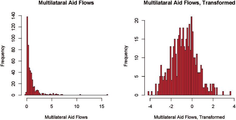
The Problem with Robust Standard Errors                         167

first estimate the MLE ^ and calculate the Hessian P. We then estimate M based on the type of
misspecification we would like to test for. In the cluster-robust case, Mc is estimated by summing
first within clusters and then over the clusters:
                                       "                              #
                                         Xn X
                                Mc ¼                     ^ gi ðYi jyÞ
                                                 gi ðYi jyÞT       ^ ;
                                             j¼1 i2cj

where c is the cluster index. In the autocorrelation-robust case, Ma adds a weight to each square of
the gradient, depending on the lag the modeler expects to exist in the data:
                                                1X n X n
                                     Ma ¼                 wjijj g^ i g^ j ;
                                                n i¼1 j¼1

where g^ is the estimated gradient. The equation for the weight vector w depends on what type of
autocorrelation-robust variance matrix the researcher wants to estimate. For example, Newey and
                                        l

                                                                                                       Downloaded from http://pan.oxfordjournals.org/ at Harvard Library on May 25, 2015
West (1987) use a weight vector 1  Lþ1   , where l is the lag i – j and L is the maximum lag.
  Once the appropriate choice of M has been made and it is calculated from the data and specified
model, we calculate the test statistic:
                                                 1 X  n
                                         D^ ij ¼ pffiffiffi    ^ ij þ P^ ij Þ:
                                                        ðM
                                                  n i¼1

     To bootstrap the variance matrix for this test statistic, we draw nb samples from the data-
generating process of the model, fðyi jÞ.  ^ For each new sample, we calculate the new MLE
^ b and the bootstrapped test statistic D^ b . Last, we estimate V^B with

                                           1 X  B
                                V^ B ¼             ðD^ b  DÞðD^ b  DÞ0 ;
                                         B  1 b¼1
             P
where D ¼ B1 Bb¼1 D^ b .
                                                             1
  Finally, this leads to our GIM test statistic oB ¼ D^ 0 V^B D,^ from which we calculate p-values
by bootstrapping.

4.3   Validation
We now evaluate the GIM test by conducting formal Monte Carlo simulations. To do this, we first
simulate data from a univariate normal distribution with mean  ¼ 5Z þ X þ Z2 and variance 1.
(We draw covariates X and Z from a bivariate normal with means 8 and 5, variances 1, and
correlation 0.5.) We then draw 100 samples with n ¼ 200 from this data-generating process, run
the GIM test on each, and obtain a p-value. Since the model is correctly specified, a formal indi-
cation of whether the GIM test is working properly would be that the computed p-values are
uniformly distributed. Figure 1 graphs the cumulative distribution of these results (plotting the
percent of p-values less than each given value of the probability). The uniform distribution of
p-values does indeed show up in the simulations and is reflected in the figure by the blue line
closely approximating the 45-degree line.
   We then evaluate the GIM test further by introducing different levels of misspecification into the
model and observing whether the test deviates as it should from uniform. We create these
misspecifications by taking the dependent variable to the power of  before running the GIM
test. In this simulation, larger values of Y will have a higher variance. We run the GIM test
for  ¼ f1; 3; 4; 5g and report results in Fig. 1 (in blue, green, orange, and brown, respectively).
All misspecified simulations  > 1 have p-values above the 45-degree line, indicating that the
p-values are not uniformly distributed, and indeed, as expected  grows, the results are skewed
more toward lower, less uniform p-values. Higher levels of misspecification have a higher p-value
line because the test has more power to detect this misspecification.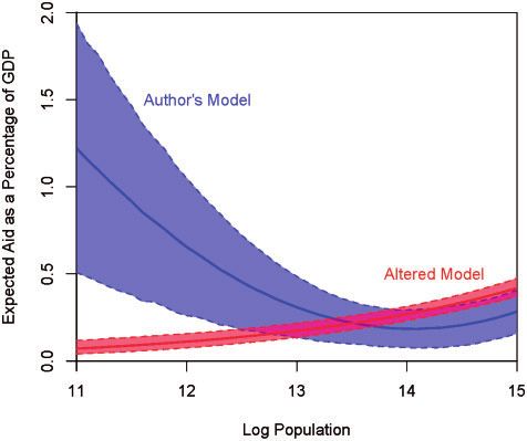
168                                 Gary King and Margaret E. Roberts

                                                                                                          Downloaded from http://pan.oxfordjournals.org/ at Harvard Library on May 25, 2015
Fig. 1 Cumulative distribution of p-values from the GIM test for correctly specified datasets, and from
increasingly misspecified datasets.

4.4    Limitations
The difference between robust and classical standard errors, and the more formal GIM test,
provides important clues, but of course cannot reveal all possible problems. No one type of
robust standard errors is consistent under all types of misspecification, and so no one such differ-
ence is a diagnostic for everything. As commonly recommended, many different tests and diagnostic
procedures should be used to evaluate whether the assumptions of the model are consistent with the
data. And even then, problems can still exist; for example, omitted variables that do not induce
heteroskedasticity in the residuals, but are still important, can bias estimates in ways that no robust
estimator can pick up. Indeed, this approach will also detect problems of endogeneity, measure-
ment error, missing data, and others that are not reflected in the evidence. As such, any inference
must always rely on some theoretical understanding. Nevertheless, these qualifications do not
absolve researchers from checking whatever can be checked empirically, as we show how to do here.

5     Simulations
Although our GIM test offers a formal evaluation and decision rule for the difference between
robust and classical standard errors, we now develop some intuition by showing how the GIM test
compares to the rule-of-thumb difference between robust and classical standard errors, using simu-
lations with various misspecified functional forms.
   For intuition, we offer here three Monte Carlo experiments of the general analytical results
summarized in Section 2. We set up these experiments to highlight common important issues,
and to also presage, and thus parallel, the empirical data we analyze, and articles we replicate,
in Section 6.

5.1    Incorrect Distributional Assumptions
In this first simulation, we use a linear-normal model to analyze data from a skewed, non-normal
process, and show how the more data deviate from the normal, the larger the differences between
robust and classical standard errors and, simultaneously, the more our GIM test reveals a problem.
Either way of looking at the results should clearly alert the investigator to a problem.
The Problem with Robust Standard Errors 169
Downloaded from http://pan.oxfordjournals.org/ at Harvard Library on May 25, 2015
Fig. 2 Incorrect distributional form simulation: robust and classical standard errors diverge (on the vertical
axis, bottom), and the GIM test rejects more (vertical axis, top), when the degree of misspecification is
larger (as indicated by the value of on the horizontal axis).
To be more specific, we draw a random variable from a normal distribution with mean
¼ 5Z þ X þ X2 . We then create the dependent variable by taking its power to a fixed parameter
. For larger values of the exponent, the distribution will be highly skewed, with a long right tail.
For n ¼ 1000, we draw the two explanatory variables X and Z from a bivariate normal with
mean parameters 8 and 5, variance 1, and correlation 0.5. Then, for each value of the parameter
from 1 to 3 (in increments of 0.002), we draw a normal random variable M from a normal distri-
bution with mean ¼ 5Z þ X þ X2 , variance 1, and then create Y ¼ M . We then run a linear
regression of Y on X, X2, and Z and calculate robust and classical standard errors.
Figure 2 then gives results for each different degree of misspecification, as indicated by the value
of on the horizontal axis plotted by the difference between the classical and robust standard error
for the coefficient on the X2 term (at the bottom of the figure on the vertical axis) and for the
percent of GIM tests rejected (in the top portion of the figure). As is evident, the difference between
robust and classical standard errors becomes dramatically different as the model becomes more
misspecified (i.e., for larger values of , to the right of the graph).
5.2 Incorrect Functional Forms
We now study what happens when the systematic component of the normal model is misspecified.
To do this, we generate the data from a linear-normal model with EðYi jXÞ i ¼
0 þ 1 Zi þ 2 Xi þ 3 X2i , but where the analyst omits X2i , effectively setting 3 ¼ 0. The amount
of misspecification is thus indicated by the value of 3 used to generate the data. For each data set,
we calculate the difference between the robust and the classical standard errors, as well as the GIM
test, and show how both clearly reveal the misspecification.
For n ¼ 1000, we create two explanatory variables X and Z from a bivariate normal with means
3 and 1, variance 1, and correlation 0.5. Then, for values of 3 from 0 to 5 in increments of 0.005,
we draw Y from a normal with mean 5Zi Xi þ 3 X2i and homoskedastic variance ( 2 ¼ 1). For
each, we run a linear regression of Y on a constant, X and Z (i.e., excluding X2).
For each of these simulated data sets, Fig. 3 plots the difference between classical and robust
standard errors on the vertical axis (bottom) and GIM test (top) by the degree of misspecification
indicated by 3 on the horizontal axis. For simulations from exactly or approximately at the correct170 Gary King and Margaret E. Roberts
Downloaded from http://pan.oxfordjournals.org/ at Harvard Library on May 25, 2015
Fig. 3 Incorrect functional form simulation. The difference between classical and robust standard errors
(bottom) and percent of GIM tests rejected (top) indicates little problem with misspecification (at the left of
the graph), but bigger differences reveal the misspecification as it gets worse (toward the right).
data-generation process (on the left), there is little deviation between robust and classical standard
errors. However, as the misspecification grows, the standard error difference and the percent of
GIM tests rejected grows fast, unambiguously revealing the misspecification. A scholar who used
one of these tests would not have a difficult time ascertaining and fixing the cause of the problem.
5.3 Incorrect Stochastic Component
For the third simulation, we generate data from a negative binomial regression model, but estimate
from its limiting case, a Poisson. The Poisson model is heteroskedastic to begin with (with mean
equal to the variance), and so this is a case of misspecification due to overdispersion, where the
variance is greater than the mean (King 1989b).
We begin with n ¼ 1000 draws of two explanatory variables X and Z from a bivariate normal
with mean 0, variance 1, and correlation 0.5. We then draw Y conditional on X from a negative
binomial distribution with mean parameter EðYi jXÞ i ¼ exp ð1 þ 0:1 Zi 0:1 Xi Þ and over-
dispersion parameter such that VðYi jXÞ ¼ i ð1 þ yi Þ, such that y > 0 and the larger is the more
the data-generation process diverges from the Poisson. For each data set, we run an exponential
Poisson regression of Y on X and Z and compare the classical and robust standard errors.
Figure 4 gives the results, with the difference in standard errors (bottom) and percent of GIM
tests rejected (top) on the vertical axis and the degree of overdispersion (misspecification) on the
horizontal axis. As is evident, robust and classical standard errors are approximately equal when
the data are nearly Poisson but diverge sharply as overdispersion increases. Thus, we have a third
example of being able to easily detect misspecification with robust and classical standard errors.
6 Empirical Analyses
We now offer three empirical examples where robust and classical standard errors differ and thus
clearly indicate the presence of misspecification, but where this issue has gone unnoticed. These
correspond to the three sections in Section 5. We then apply our more general GIM test and some
of the other standard diagnostic techniques to detect the cause of the problem, respecify the model,
and then show how the standard error differences vanish. We highlight the large differences in
substantive conclusions that result from having a model that fits the data.The Problem with Robust Standard Errors 171
Downloaded from http://pan.oxfordjournals.org/ at Harvard Library on May 25, 2015
Fig. 4 Incorrect stochastic component simulation. The vertical axis gives the difference between the clas-
sical and the robust standard errors (bottom) and percent of GIM tests rejected (top). The horizontal axis
gives , the degree of overdispersion. The larger is, the more misspecification exists in the data.
In all cases, we try to stick close to our intended purpose, and so do not explore other potential
statistical problems. We thank the authors for making their data available and making it easy to
replicate their results; none should be faulted for being unaware of the new methodological points
we make here, developed years after their articles were written. All data and information necessary
to replicate our results appear in a Dataverse replication file at King and Roberts (2014).
6.1 Small Country Bias in Multilateral Aid
We begin by replicating the analysis in Neumayer (2003, Table 3, Model 4), who argues that
multilateral aid flows (from a variety of regional development banks and United Nations
agencies as a share of total aid) favor less populous countries. The original analysis is a linear
regression of multilateral aid flows on log population, log population squared, gross domestic
product (GDP), former colony status, the distance from the Western world, political freedom,
military expenditures, and arms imports.
The robust standard errors from this regression are starkly different from the classical standard
errors. For example, for the coefficient on log population of 3.13, the robust standard error is
almost twice that of the classical standard error (0.72 versus 0.37, respectively). We can also
compare the entire robust variance matrix with the classical variance matrix, using the test we
develop in Section 4. In this case, the p-value of this test is nearly zero (172 Gary King and Margaret E. Roberts
Downloaded from http://pan.oxfordjournals.org/ at Harvard Library on May 25, 2015
Fig. 5 Distribution of the dependent variable before (left) and after (right) the Box-Cox transformation.
Fig. 6 Evaluations of the original model (top row) and our alternative model (bottom row), for both
residual plots (left column) and QQ plots (right column).
Two other diagnostics we offer in Fig. 6 are similarly revealing. The top left panel is a plot of
the residuals from the author’s model on the vertical axis by log population on the horizontal.
The result is an almost textbook example of heteroskedasticity, with very low variance on the
vertical axis for small values of log-population and much higher variance for large values. After
taking the log, the result at the bottom left is much closer to homoskedastic. We also conduct a test
for normality via a Q-Q plot for the original model (top right) and the model applied to theThe Problem with Robust Standard Errors 173
Downloaded from http://pan.oxfordjournals.org/ at Harvard Library on May 25, 2015
Fig. 7 Aid flows and country size: quadratic in the original misspecified model, but monotonically
increasing in the revised model that passes the specification tests.
transformed data (bottom right), which leads us to the same conclusion that our modified model
has corrected the misspecification. Finally, we note that the GIM test is now not significant (p-value
of 0.51).
For all these tests, the problem revealed by the difference between the classical and the robust
standard errors has been corrected by the transformation. At this point, the theory (i.e., the full
model) has been adjusted so that the observable implications of it, which we are able to measure,
are now consistent with the data, the result being that we should be considerably more confident
in the empirical results, whatever they are. In the present case, however, it happens that the sub-
stantive results did change quite substantially.
Neumayer (2003) writes, “as population size increases, countries’ share of aid initially falls
and then increases. Multilateral aid flows thus exhibit a bias toward less populous countries.”
We replicate this quadratic relationship and represent it with the blue line and associated confidence
region in Fig. 7. However, as we show above, the robust and classical standard errors indicate
the model is misspecified. In the model that passes this specification test, which we display in red,
the results are dramatically different: now the bias in aid flows is clearly to countries with larger
populations, for the entire range of population in the data.
6.2 The Effects of Trade Agreements on Foreign Direct Investment
For our second example, we replicate Büthe and Milner (2008, Table 1, Model 4), who argue that
having an international trade agreement increases foreign direct investment (FDI). Their analysis
model is linear regression with time-series cross-sectional data and intercept fixed effects for
countries, using cluster-robust standard errors. Their dependent variable is annual inward FDI
flows, and their independent variables of interest are whether the country is a member of the
General Agreement on Tariffs and Trade through the World Trade Organization (GATT/WTO)
and the number of preferential trade agreements (PTAs) a country is party to.
We focus on the (1.08) coefficient on GATT/WTO membership for which the classical standard
error is 0.21, and the cluster-robust standard error is almost twice as large, at 0.41. The GIM test
calculating the difference between the Discroll-Kraay autocorrelation consistent and classical
variance matrices indicates a significant difference between the two matrices (with a p-value of174 Gary King and Margaret E. Roberts
Fig. 8 Comparison of detrending strategies: raw data (left), the Büthe and Milner (2008) attempt at linear
detrending (center), and our quadratic detrending (right).
Downloaded from http://pan.oxfordjournals.org/ at Harvard Library on May 25, 2015
We applied the usual regression diagnostics and find that the source of the misspecification is the
authors’ detrending strategy. Büthe and Milner (2008) detrend because “the risk of spurious cor-
relation arises when regressing a dependent variable with a trend on any independent variable with
a trend.” This is an excellent motivation, and the authors clearly followed or improved best prac-
tices in this area. However, they detrend each variable linearly, even though many of the trends are
unambiguously quadratic, and they restrict the trend to be the same for all nations, which is also
contrary to the evidence in their highly heterogeneous set of countries. The result is that their
detrending strategy induced a new spurious time-series pattern in the data.
For mean cumulative PTAs and FDI inflows over time, Fig. 8 presents the raw data in a time-
series plot on the left. As the authors note, using data with trends like this can lead to spurious
relationships. They detrend both time series linearly, which we represent in the center figure and
which, unfortunately, still has a very pronounced trend. In some ways, this induces an even stronger
(spurious) relationship between these two variables. Our alternative specification detrends
quadratically by country, illustrated in the right graph, which results in transformed variables
that are much closer to stationary. Further, the GIM test for heteroskedasticity and autocorrelation
is no longer significant (the p-value is 0.35).7
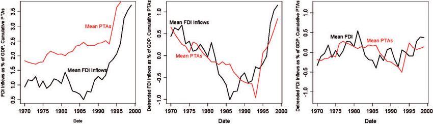
We provide more intuition for the exact source of the problem in Fig. 9 by plotting the residuals
(and a smoothed loess line) over time for three example countries. We do this for the original model
(in black) and our modified model that detrends quadratically by country (in red). The fact that
individual countries exhibit such clear differences in time-series patterns reveals where the difference
between cluster-robust and classical standard errors is coming from in the first place. That is, the
problem stems from the fact that the authors restricted the detrending to be the same in every
country, when in fact the time-series pattern varies considerably across countries. Our alternative
approach of modeling the patterns in the data produces residuals with time-series patterns that are
closer to stationary and similar across these regions, and as a result the robust and classical
standard errors are now much closer. Changing to a better-fitting functional form parallels our
simulation in Section 5.2.
To supplement the three examples in Fig. 9, we present in Fig. 10 loess smoothed lines fit
to residuals for each country, all together (standardized by country so they can appear in
7
We note that some constructions of the GIM test (testing cluster-robust without time versus normal variance-covariance
matrix, e.g.) still show some differences. Thus, although this new model is considerably less misspecified than the
original, there may exist an even better model we have not yet discovered; this new model might provide different
results but may also reflect a problem in these data with “model dependence” that could also use some attention (e.g.,
King and Zeng 2006). To optimize for the expository purposes of this methods paper, we followed the procedure of
substantially reducing misspecification in authors’ model while changing other assumptions as little as possible. An
alternative and probably more substantive approach would be to drop the detrending strategy altogether and to model
the time-series processes in the data more directly.The Problem with Robust Standard Errors 175
Fig. 9 Time-series residual plots for three sample countries: original model (dark) and modified model
Downloaded from http://pan.oxfordjournals.org/ at Harvard Library on May 25, 2015
(light), with dots for residuals and loess smoothed lines.
Fig. 10 Standardized residuals for all included countries: original model (left) and our modified model
(right).
one graph). While many countries show strong nonlinear residual trends in the original speci-
fication (left panel), most of the trends in our alternative specification have now vanished (right
panel).
We conclude by noting that the conclusions of the authors change considerably. Unlike in the
original model, neither of the two variables of interest (GATT/WTO or PTAs) are still significantly
correlated with FDI inflow. Figure 11 gives one visualization of this relationship, showing both the
elimination of the key result and the fact that robust and classical standard errors differ dramat-
ically in the authors’ original model but after adjustment they are approximately the same. As is
obvious from the country-level results, estimates of numerous country-level quantities would also
differ between the two models.
We followed a detrending strategy here to stay as close as possible to the analytic strategy in the
original paper, but other approaches may be preferable for the substantive purpose of estimating
the impact of trade agreements on FDI inflows. In particular, some of the variation attributed to
uncertainty by these modeling approaches may be due to heterogeneous treatment effects, as at
least some interpretations of our auxiliary analyses (not shown) may suggest. That is, it may be that
trade agreements have a positive relationship with FDI inflows in some countries (e.g., Colombia)
and a negative one in others (e.g., the Philippines).You can also read