PREDICTION OF PATHOLOGIES OF HUMAN NOSE BY MACHINE LEARNING WITH FLOW PHYSICS
←
→
Page content transcription
If your browser does not render page correctly, please read the page content below
Master’s Thesis     Academic Year 2020-2021

      PREDICTION OF PATHOLOGIES
OF HUMAN NOSE BY MACHINE LEARNING
           WITH FLOW PHYSICS

             Kazuto HASEGAWA
             (Student ID: 936079)

Academic supervisor: Prof. Maurizio QUADRIO

           POLITECNICO DI MILANO
Master of Science in AERONAUTICAL ENGINEERING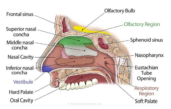
Abstract
Computational fluid dynamics is expected to play a crucial role to diagnose a condition
of human nose. The detailed information and solutions provided by numerical simula-
tions enable us to not only analyze flow characteristics but also visualize flow fields in
an understandable manner. However, it is also true that we often have to include ex-
perted knowledge to achieve a precise assessment since there are considerable uncertain-
ties caused by the difficulty of diagnosis for human nose. We here consider the use of
data-driven frameworks for diagnosing nasal pathologies. Geometries and flow fields of
200 different noses, half of them exhibit some degree of turbinate hypertrophy, are utilized
to predict their pathological parameters. First, the geometrical characteristics of the noses
are extracted as a functional map between a reference healthy nose and other noses. The
functional maps are then used to train neural networks and to predict pathological param-
eters. Three different machine learning models with different inputs and configurations
are trained to examine the predictability of the methods for the pathologies. In addition to
the prediction based on the geometric information, we also consider the utilization of flow
measurements such as pressure and wall shear stress. The flow fields are considered as
a function defined on nose which can be expressed by linear combinations of eigenfunc-
tions of Laplace-Beltrami operator. The present results show reasonable agreements with
the reference pathologies. We also find that the prediction performance can significantly
be improved by including flow information as the input of machine learning models.
Acknowledgments

I really appreciate the grateful support from my supervisor, Professor Maurizio Quadrio.
He kindly welcomed me and gave me the opportunity to work on this project. Even after
I was forced to return to Japan due to COVID-19, he supported my remote study.
    I would also like to express my gratitude to Professor Koji Fukagata for giving me the
opportunity to study at Politecnico di Milano.
    I am really grateful to the kind support from Mr. Andrea Schillaci. He gave me a lot
of support. Despite the time difference, he was always available for meetings and fruitful
discussions.
    At last, I would like to thank my family for allowing me to study abroad at Politecnico
di Milano and for their constant support during my stay.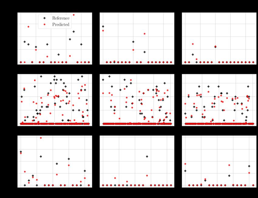
Contents

List of Figures                                                                                                                 iii

List of Tables                                                                                                                  vi

1   Introduction                                                                                                                 1
    1.1 OpenNOSE project . . . . . . . . . . . . . . . . . . . . . . . . . . . . .                                               1
    1.2 Background and objective . . . . . . . . . . . . . . . . . . . . . . . . .                                               1

2   Modeling and Numerical Simulation of Nasal Cavity                                                                            4
    2.1 Nasal cavity and turbinate hypertrophies . . . . . . . . . . . . . . . . . .                                             4
    2.2 Simplified model for simulations . . . . . . . . . . . . . . . . . . . . . .                                             5
    2.3 Numerical simulations . . . . . . . . . . . . . . . . . . . . . . . . . . .                                              7

3   Machine Learning Techniques                                                                                                  9
    3.1 Linear regression . . . . . . . . . . . . . . . . .                 .   .   .   .   .   .   .   .   .   .   .   .   .    9
        3.1.1 Lasso . . . . . . . . . . . . . . . . . . .                   .   .   .   .   .   .   .   .   .   .   .   .   .    9
    3.2 Neural networks . . . . . . . . . . . . . . . . . .                 .   .   .   .   .   .   .   .   .   .   .   .   .   10
        3.2.1 Neural network models . . . . . . . . . .                     .   .   .   .   .   .   .   .   .   .   .   .   .   11
        3.2.2 Activation function . . . . . . . . . . . .                   .   .   .   .   .   .   .   .   .   .   .   .   .   12
        3.2.3 Loss function . . . . . . . . . . . . . . .                   .   .   .   .   .   .   .   .   .   .   .   .   .   14
        3.2.4 Optimizer . . . . . . . . . . . . . . . . .                   .   .   .   .   .   .   .   .   .   .   .   .   .   15
        3.2.5 Backpropagation . . . . . . . . . . . . .                     .   .   .   .   .   .   .   .   .   .   .   .   .   18
        3.2.6 Training and evaluation . . . . . . . . . .                   .   .   .   .   .   .   .   .   .   .   .   .   .   19
        3.2.7 Major problems in neural network models                       .   .   .   .   .   .   .   .   .   .   .   .   .   20
        3.2.8 Batch normalization . . . . . . . . . . .                     .   .   .   .   .   .   .   .   .   .   .   .   .   22
        3.2.9 Dropout . . . . . . . . . . . . . . . . . .                   .   .   .   .   .   .   .   .   .   .   .   .   .   22
        3.2.10 Cross validation . . . . . . . . . . . . .                   .   .   .   .   .   .   .   .   .   .   .   .   .   22

4   Functional Maps                                                                                                             25
    4.1 Functional map representation . . .     .   .   .   .   .   .   .   .   .   .   .   .   .   .   .   .   .   .   .   .   25
    4.2 Functional map inference . . . . . .    .   .   .   .   .   .   .   .   .   .   .   .   .   .   .   .   .   .   .   .   27
        4.2.1 Function preservation . . . .     .   .   .   .   .   .   .   .   .   .   .   .   .   .   .   .   .   .   .   .   28
        4.2.2 Operator commutativity . .        .   .   .   .   .   .   .   .   .   .   .   .   .   .   .   .   .   .   .   .   29
        4.2.3 Estimating functional maps        .   .   .   .   .   .   .   .   .   .   .   .   .   .   .   .   .   .   .   .   29

                                            i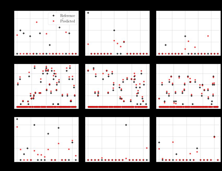
5   Prediction with machine learning models                                                                    30
    5.1 Prediction from functional maps . . . . . . . . . . .      .   .   .   .   .   .   .   .   .   .   .   30
         5.1.1 Data preparation . . . . . . . . . . . . . . .      .   .   .   .   .   .   .   .   .   .   .   30
         5.1.2 Model configuration and learning conditions         .   .   .   .   .   .   .   .   .   .   .   33
         5.1.3 Results . . . . . . . . . . . . . . . . . . . .     .   .   .   .   .   .   .   .   .   .   .   38
    5.2 Prediction from flow field and geometry . . . . . . .      .   .   .   .   .   .   .   .   .   .   .   42
         5.2.1 Data preparation . . . . . . . . . . . . . . .      .   .   .   .   .   .   .   .   .   .   .   42
         5.2.2 Model configuration and learning conditions         .   .   .   .   .   .   .   .   .   .   .   48
         5.2.3 Results . . . . . . . . . . . . . . . . . . . .     .   .   .   .   .   .   .   .   .   .   .   49
    5.3 Discussion . . . . . . . . . . . . . . . . . . . . . . .   .   .   .   .   .   .   .   .   .   .   .   51

6   Conclusions                                                                                                53

Reference                                                                                                      55

                                            ii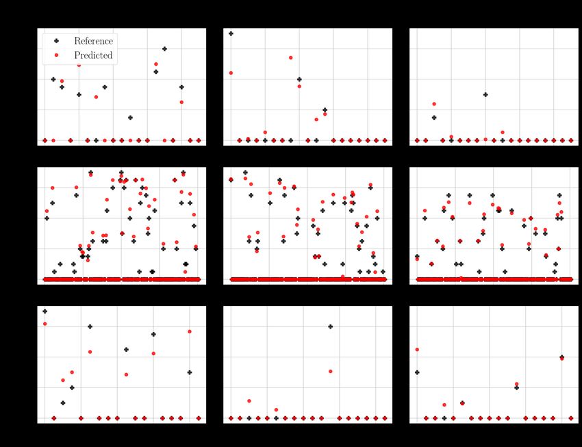
List of Figures
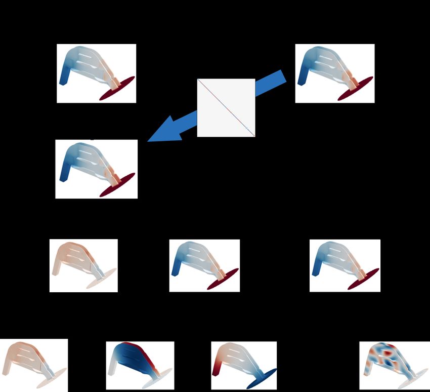
2.1 Schematic of nasal cavity (1) The Respiratory System. (n.d.). . . . . . . . 5
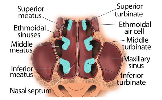
2.2 Schematic of nasal cavity (2) (The Respiratory System., n.d.). . . . . . . . 6
2.3 Model shape (Romani, 2017). . . . . . . . . . . . . . . . . . . . . . . . 6
3.1 Operations in the convolutional layer and the sampling layer: (a) con-
volutional operation using a weighted filter W; (b) the computation in the
convolution layer with M = 3; (c) max pooling operation. (d) upsampling
operation. . . . . . . . . . . . . . . . . . . . . . . . . . . . . . . . . . . 12
3.2 Activation functions. . . . . . . . . . . . . . . . . . . . . . . . . . . . . 13
3.3 An example of training and validation loss history of the overfitted model. 21
3.4 Dropout neural net model. (a): A standard neural net with 2 hidden layers.
(b): An example of a thinned net produced by applying dropout to the
network on (a). Crossed units have been dropped. (Srivastava et al., 2014) 23
3.5 An example of fivefold cross validation. The blue boxes indicate training
data used for deriving machine learning model.The red boxes indicate test
data used to obtain test scores. An average score of five test scores are
used for the optimization procedure and assessment (Fukami, Fukagata
and Taira, 2020). . . . . . . . . . . . . . . . . . . . . . . . . . . . . . . 23
4.1 The schematic for the functional maps (Ovsjanikov et al., 2017). When
the functional spaces of source and target shapes M and N are endowed
with bases ϕM and thus every function can be written as a linear combina-
tion of basis functions, then a linear functional map TF can be expressed
via a matrix C that intuitively translates the coefficients from one basis
to another. . . . . . . . . . . . . . . . . . . . . . . . . . . . . . . . . . . 26
5.1 Mapping a function defined on the reference nose onto each target nose
by corresponding functional map. The color scale on noses represents the
function. The functional maps are computed between the healthy refer-
ence nose and the other noses. . . . . . . . . . . . . . . . . . . . . . . . 31
5.2 An example of the correspondences encoded in the functional map. The
function to highlight the inferior turbinate defined on the left reference
nose are mapped onto the right pathological nose. . . . . . . . . . . . . . 32
5.3 The examples of 20×20 functional maps. The heat map represent the val-
ues of the matrix, i.e., functional map. The values above the heat map are
the pathological parameters for inferior turbinate head, inferior turbinate
body and middle turbinate head. . . . . . . . . . . . . . . . . . . . . . . 32
iii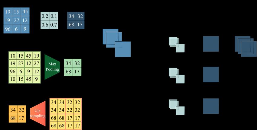
5.4    The algorithms to construct the machine learning models. (a): The blocks
       used in the models. The “Conv(3, 3)”, “BN” and “FC(n)” in the blocks
       denote the convolution layer with 3 × 3 filter, batch normalization layer
       and fully-connected layer, which is a layer of the perceptrons, with n per-
       ceptrons. (b): The diagram of the CNN model. The “size” in the diagram
       represents the size of data, and “unit” is variable for “FC block”. (c):
       The MLP model structure. In this mode, the functional maps fed into the
       model are flatten to input “FC block”. (d): The schematics to construct
       the SVD model. The singular values of the functional maps are computed
       and input to “FC block”. The “num layer” is the number of layers of the
       model. . . . . . . . . . . . . . . . . . . . . . . . . . . . . . . . . . . . .           34
5.5    The example of the history of the training and validation loss of the CNN
       model with 20 × 20 functional maps. . . . . . . . . . . . . . . . . . . . .              35
5.6    The dependencies on the size of the input functional maps and the model
       configuration. The fivefold cross-validation is performed. The error bar
       represents the standard deviation of the validation loss with respect to
       each fold. . . . . . . . . . . . . . . . . . . . . . . . . . . . . . . . . . .           36
5.7    The predictions of the CNN model with the 20 × 20 functional maps. The
       column represents the pathological parameters and the row is the kind of
       data. The values above the scatter plots indicate the mean squared errors. .             37
5.8    The predictions of the MLP model with the 20 × 20 functional maps. The
       column represents the pathological parameters and the row is the kind of
       data. The values above the scatter plots indicate the mean squared errors. .             38
5.9    The predictions of the SVD model with the 20 × 20 functional maps. The
       column represents the pathological parameters and the row is the kind of
       data. The values above the scatter plots indicate the mean squared errors. .             39
5.10   The mean squared errors of the test data against the pathological param-
       eters and models. The (1), (2) and (3) denote the pathological param-
       eters for the inferior turbinate head, inferior turbinate body and middle
       turbinate head, respectively. . . . . . . . . . . . . . . . . . . . . . . . . .          40
5.11   The confusion matrixes of the predictions for each pathology and model. .                41
5.12   The schematic of the data preparation. (a): The pressure on the tar-
       get nose pt is mapped onto the reference nose as b           pt . (b): The pressure
       difference ∆b     pt between the pressure of the reference nose pr and the
       mapped pressure b        pt is computed on the reference nose. (c): The pres-
       sure difference ∆b       pt is assumed to be the linear combination of the eigen-
       functions of the reference nose B = {b1 , b2 , · · · , bn } and its coefficients
       γ = {γ1 , γ2 , · · · , γn }T . . . . . . . . . . . . . . . . . . . . . . . . . . . . .   43
5.13   Dependence of reconstruction ability on the number of the bases used to
       reconstruct field. The chart represents the mean squared errors against
       the number of the bases, averaged also over all target noses. The color
       scale on the 3D plots of nose are the reference and reconstructed pressure
       difference fields of a target nose. The values above the 3D plots denote
       (the number of bases): (the mean squared error of the presented pressure
       difference). . . . . . . . . . . . . . . . . . . . . . . . . . . . . . . . . .            44

                                              iv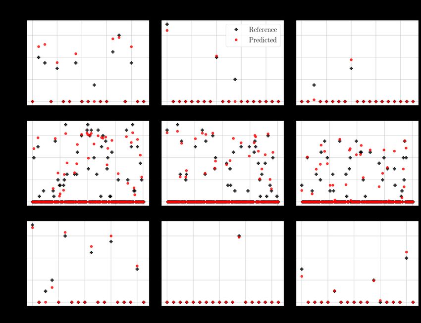
5.14 Dependence of reconstruction ability on the number of the bases used to
     reconstruct field. The chart represents the mean squared errors against
     the number of the bases, averaged also over all target noses. The color
     scale on the 3D plots of nose are the reference and reconstructed wall
     shear stress difference fields of a target nose. The values above the 3D
     plots denote (the number of bases): (the mean squared error of the WSS
     difference). . . . . . . . . . . . . . . . . . . . . . . . . . . . . . . . . .     44
5.15 The examples of the coefficients γ of 200 bases for pressure. The values
     above the plots are the pathological parameters for inferior turbinate head,
     inferior turbinate body and middle turbinate head. . . . . . . . . . . . . .      45
5.16 The examples of the coefficients γ of 200 bases for wall shear stress.
     The values above the plots are the pathological parameters for inferior
     turbinate head, inferior turbinate body and middle turbinate head. . . . . .      45
5.17 The model configuration for prediction the pathologies from the coeffi-
     cients γ. The blocks used in this figure are defined in figure 5.4. . . . . .     46
5.18 The dependency on the number of the bases. The fivefold cross-validation
     is performed. The error bar represents the standard deviation. . . . . . . .      47
5.19 The predictions of the model trained by the coefficients γ of pressure. The
     column represents the pathological parameters and the row is the kind of
     data. The values above the scatter plots indicate the mean squared errors. .      48
5.20 The predictions of the model trained by the coefficients γ of wall shear
     stress. The column represents the pathological parameters and the row
     is the kind of data. The values above the scatter plots indicate the mean
     squared errors. . . . . . . . . . . . . . . . . . . . . . . . . . . . . . . . .   49
5.21 The confusion matrixes of the predictions for each pathology by pressure
     and wall shear stress. . . . . . . . . . . . . . . . . . . . . . . . . . . . .    50

                                          v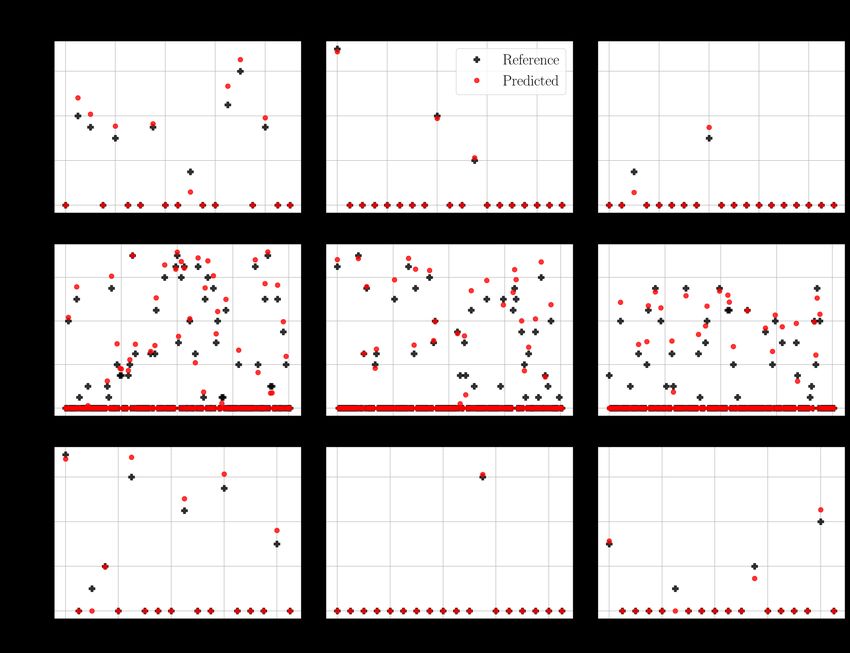
List of Tables

 2.1   The variations of nose geometry. . . . . . . . . . . . . . . . . . . . . . .    7

 5.1   The accuracies of the predictions. . . . . . . . . . . . . . . . . . . . . .    42
 5.2   Accuracy. . . . . . . . . . . . . . . . . . . . . . . . . . . . . . . . . . .   50

                                          vi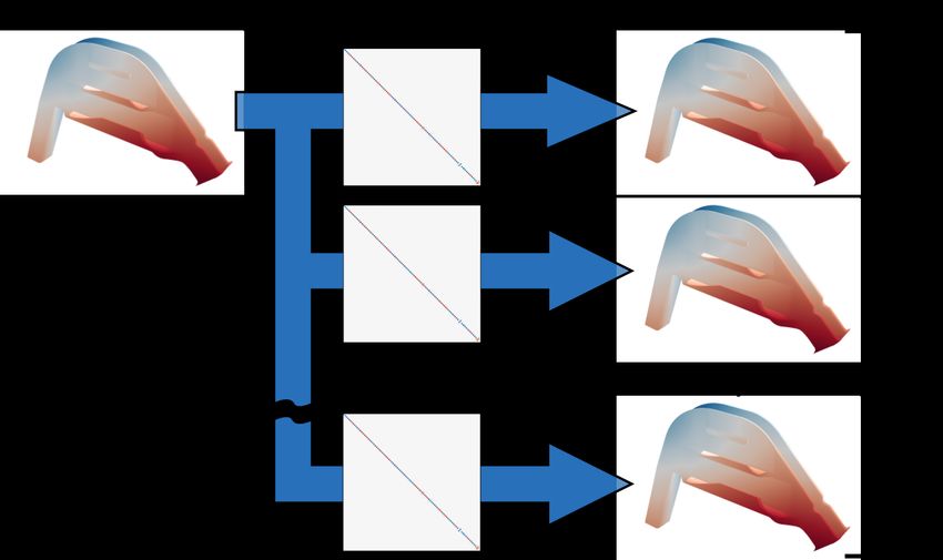
Chapter 1

Introduction

1.1     OpenNOSE project

The objective of OpenNOSE project is to create a reliable, patient-specific and open

source tool to help diagnose and study nasal conditions. Most of the previous works of
this project have focused on reproducing and analysing airflows inside the human nasal
cavity by using computational fluid dynamics (CFD) (Saibene et al., 2020; Covello et al.,

2018). As a results, the nasal airflow close to an practice one is reasonably simulated with
some limitations (Quadrio et al., 2014). The next step of this project is then the utiliza-
tion of CFD solutions for diagnosing the nasal pathologies. One of the works related to

this step is performed by Schillaci et al. (2021). Schillaci et al. (2021) inferred the ge-
ometries of airfoils and nasal structures, i.e., pathological parameters, from flow features
through simple fully-connected neural network models. The present study aims to predict

the nasal pathologies from nose geometries and fluid dynamics features assuming that
the CFD solutions provide a reasonable solution to improve the predictions, as a part of
OpenNOSE project. The detailed background and objective of this study are offered in

what follows.

1.2     Background and objective

CFD, which simulates flows by numerically solving the governing equations for the mo-
tion of fluids, has exhibited a great capability in assessing the detailed information in a

system of a wide range of science and engineering thanks to the development of compu-

                                             1
tational power. The medical field is, of course, not an exception for the application of
them (Saibene et al., 2020; Covello et al., 2018). Zhao et al. (2004) developed a method
to quickly convert nasal CT scans from an individual patient into an anatomically accu-
rate 3-D numerical nasal model using CFD. The effects of nasal obstruction with swelling
of inferior turbinates on the aerodynamic flow pattern are investigated with turbulence
models (Chen et al., 2010). These CFD results are expected to be useful to diagnose
human systems in an interpretable manner with the flow visualization. However, even
though with the development of CFD in the medical field, diagnosing the human system
is very challenging because the important information for the diagnosis cannot be pro-
vided directly by CFD solutions themselves, which implies that the incorporation of a
priori knowledge by experts should be required for precise assessments. Particularly, the
diagnosis of nasal breathing difficulties (NBD), an pathological condition of human nose
that often requires corrective surgery, is known as a longstanding and challenging matter.
Some previous studies have reported that the failure rate of surgery is up to 50% (Sundh
and Sunnergren, 2015; Illum, 1997). Although the CFD solutions of the nasal airflow is
considered to be effective for the diagnosis of NBD, a new framework, that can help the
reasonable diagnosis while incorporating the accumulated knowledge as a database, has
been eagerly desired.
Of particular interest here is the utilization of machine learning techniques which have
recently been recognized as a powerful analysis tool in assessing fluid flows. (LeCun
et al., 2015; Kutz, 2017; Brunton et al., 2020; Taira et al., 2020; Brenner et al., 2019) The
reconstruction and estimation of flow data and characteristics can be regarded as one of
main uses in machine learning for fluid mechanics (Fukami, Fukagata and Taira, 2020).
Carrillo et al. (2016) used a neural network to estimate the Reynolds number from the
information obtained by detector located in a wake flow behind two-dimensional cylin-
der. Fukami et al. (Fukami, Fukagata and Taira, 2019, 2021) performed super-resolution
reconstruction to recover a high-resolution flow field from a low-resolution counterpart
with convolutional neural network (CNN) while considering unsteady laminar wakes and
2wall-bounded turbulence. A global field reconstruction from limited sparse measurements
has also been performed with neural networks (Erichson et al., 2020; Fukami, Maulik,
Ramachandra, Fukagata and Taira, 2021). The application of machine learning for data
estimation is not only for numerical side but also for experiments. Cai et al. (2019) used
CNNs in obtaining the flow field from particle images. The aforementioned references
indicate the capability of machine learning to extract hidden relations and physics from
big data associated with fluid flows.
The objective of the present study is to predict the nasal pathologies from geomet-
rical information and flow fields simulated by CFD. The CFD data simulated by Ro-
mani (2017) are used as nasal airflows. The simplified nasal cavity model is built using
Computer-aided Design (CAD) with eight anatomical variations, five of which behave as
harmless anatomical differences between healthy individuals, while the remaining three
have a pathological impact on the airflow. To compare the results, machine learning mod-
els are constructed with two conditions in order to infer the pathological parameters. First,
the pathologies are predicted from the geometries by training three machine learning mod-
els with different structures. To extract the features from 3D shape of nose, a functional
map, proposed by Ovsjanikov et al. (2012), are utilized. We also consider the use of flow
field information such as pressure and wall shear stress to predict the pathologies. The
ability of prediction is evaluated by unseen data for the machine learning models.
3Chapter 2
Modeling and Numerical Simulation of
Nasal Cavity
The methods for numerical simulation of nasal airflows are presented in this chapter. In
this study, the flow fields simulated by Romani (2017) are used. For further details of
numerical simulations, readers refer to Romani (2017).
2.1 Nasal cavity and turbinate hypertrophies
In this section, anatomical parts of human nose and pathologies investigated in this study,
i.e., turbinate hypertrophies, are explained. The illustrations of nasal cavity are presented
in figures 2.1 and 2.2. The human nose is the olfactory organ as well as the main pathway
for air to enter and exit the lungs. The nose warms, humidifies, and cleans the air going to
the lungs. The upper part of the external nose is supported by bone, while the lower part
being supported by cartilage. The inner space of the nose is called nasal cavity, which is
divided into two passages by the nasal septum. The nasal septum is made of bone and
cartilage and extends from the nostrils to the back of the nose. Bones called nasal turbinate
protrudes into the nasal cavity. These turbinates, shown in figure 2.2, greatly increase the
surface area of the nasal cavity, thereby allowing for more effective exchange of heat and
moisture. In the upper part of the nasal cavity, there are cells called olfactory receptors.
They are specialized nerve cells equipped with hairs. The hairs of each cell respond to
various chemicals and, when stimulated, produce nerve impulses that are sent to the nerve
cells of the olfactory bulb, located in the cranium just above the nose. The nerve impulses
4Figure 2.1: Schematic of nasal cavity (1) The Respiratory System. (n.d.).
are transmitted directly from the olfactory bulb to the brain by the olfactory nerve, where
they are recognized as odors.
Turbinate hypertrophy is a type of chronic rhinitis in which the mucous membrane of
the nasal cavity, especially the inferior turbinate mucosa, is chronically swelled, resulting
in symptoms such as nasal congestion, nasal discharge, and decreased sense of smell.
It is caused by chronic irritation from allergic rhinitis, drug-induced rhinitis caused by
long-term use of over-the-counter nasal drops, and compensatory thickening of the wider
inferior turbinate due to imbalance in the width of the left and right nasal cavities caused
by nasal septal kyphosis.
2.2 Simplified model for simulations
The simplified model of the nasal cavity proposed by Romani (2017) is presented in figure
2.3. This model consists of inlet sphere, fossa, nasal valve, turbinates, central septum-like
structure, nasopharynx and laryngopharynx. To create various geometries and airflows,
5Figure 2.2: Schematic of nasal cavity (2) (The Respiratory System., n.d.).
Figure 2.3: Model shape (Romani, 2017).
6Table 2.1: The variations of nose geometry.
Variation Non-pathological or pathological
Septum lateral position non-pathological
Longitudinal position of superior meatus non-pathological
Vertical position of superior meatus non-pathological
Section change steepness at inferior meatus inlet non-pathological
Nasal valve position non-pathological
Head of inferior turbinate hypertrophy pathological
Overall inferior turbinate hypertrophy pathological
Head of middle turbinate hypertrophy pathological
eight parameters for variations of geometry are defined. The eight parameters include
five harmless anatomical differences between healthy individuals and three pathological
variations, replicating the condition known as turbinate hypertrophies described above,
as summarized in table 2.1. In this study, the last three parameters, i.e., head of inferior
turbinate hypertrophy, overall inferior turbinate hypertrophy, and head of middle turbinate
hypertrophy, are the target of the predictions. The range of variations of head of inferior
turbinate hypertrophy, overall inferior turbinate hypertrophy and head of middle turbinate
hypertrophy are set to 0.1 mm to 0.7 mm, 0.1 mm to 0.7 mm and 0.1 mm to 0.4 mm,
respectively. Note that 0 mm indicates the healthy state for each parameter.
By combining these eight modifications, 200 different geometries are generated. They
include 100 non-pathological cases and 100 combinations of turbinate hypertrophies.
2.3 Numerical simulations
In this study, the governing equations for nasal cavity flow are incompressible steady-state
Reynolds-Averaged Navier-Stokes (RANS) equations, i.e.,
∇ · u = 0, (2.1)
( ) 1
∇ · (uu) + ∇ · u′ u′ + ∇p = ν∇2 u. (2.2)
ρ
In the equations above, u, p and ρ denote the velocity vector, the pressure and the density,
and · and ·′ are the mean (time-averaged) component and the fluctuating component, e.g.,
u represent mean velocity vector and u′ velocity fluctuation. Using Reynolds decompo-
7sition, the flow velocity vector can de decomposed as
u = u + u′ . (2.3)
The term u′ u′ in equation 2.2 is called as Reynolds stress tensor and represent the effect of
the fluctuating motions in the mean flow field. To close the stress tensor term, we use k–ω
SST (Menter, 1994) model as a turbulence model. This model contains two conservation
equations: one for turbulent kinetic energy k and one for specific dissipation rate ω.
The boundary condition driving the flow into the nasal cavity is a total pressure-over-
density difference of 20 m2 /s2 between the inlet, represented by the spherical cap, and the
outlet, which is the lower face of the laryngopharynx. This condition is similar conditions
to a real nasal cavity airflow. The no-slip boundary condition is applied to the solid
boundaries and a null normal gradient condition is used for the inlet and the outlet.
The numerical simulation is performed with OpenFOAM (v1806+), a widely used
open source CFD tool. The simulation results are verified and validated by Romani
(2017).
8Chapter 3
Machine Learning Techniques
In recent years, machine learning techniques, which can automatically extract key fea-
tures from tremendous amount of data, have achieved noteworthy results in various fields
including fluid dynamics owing to the advances in the algorithms centering on deep learn-
ing (LeCun et al., 2015; Kutz, 2017; Brunton et al., 2020; Taira et al., 2020; Brenner et al.,
2019; Fukami, Fukagata and Taira, 2020), which has been enabled by the recent devel-
opment of computational power. The machine learning methods which are used in this
study are presented in this section.
3.1 Linear regression
Linear regression is a method to solve the typical linear problem,
Y = Xβ, (3.1)
where Y and X denote response variables and explanatory variable, respectively. In this
problem, we obtain the coefficient matrix β representing the relationships between Y and
X. Using the linear regression method, we can find an optimal coefficient matrix β so
that the error between the left-hand side and right-hand side is minimized:
β = argmin||Y − Xβ||2 . (3.2)
3.1.1 Lasso
Least absolute shrinkage and selection operator (Lasso) (Tibshirani, 1996) was proposed
as a sparse regression method which takes a constraint for the sparsity of the coefficient
9matrix β, i.e., some components are zero, in the minimization process. With Lasso, the
sum of the absolute value of the coefficient matrix is incorporated with the error to deter-
mine the coefficient matrix:
∑
β = argmin ||Y − Xβ||2 + α |β j | . (3.3)
j
If the sparsity constant α is set to a high value, the estimation error becomes relatively
large while the coefficient matrix results in sparse. The Lasso algorithm introduced above
has, however, two drawbacks. One of them is that the Lasso cannot select variables prop-
erly if there is a group of variables whose correlations are very high. To overcome this
issue known as the collinearity problem, elastic net (Enet) (Zou and Hastie, 2005) was
proposed. Another problem here is that the penalization methods usually show biased
estimation with a large penalty. In other words, the predictions may sometimes result
in non-optimal and do not perform well with a high sparsity parameter used to obtain a
parsimonious and sparse model. To solve this issue called the lack of oracle property, the
adaptive Lasso (Alasso) (Zou, 2006) was presented.
3.2 Neural networks
Neural network (NN) is one of the most famous and popular methods in machine learn-
ing. For instance, convolutional neural network (CNN) (LeCun et al., 1998) is able to
capture the spacial information of two- or three-dimensional data, and it has widely been
used in a wide range of scientific fields. Recurrent neural network (RNN) can process
sequences of inputs using their internal states. Due to the strength in handling sequen-
tial data such as time-series data sets, the RNN is utilized for language processing and
time series regression. However, RNN is often suffered from vanishing gradient prob-
lem, which is explained in section 3.2.7, because of its configuration. To overcome this
problem, Hochreiter and Schmidhuber (1997) proposed long-short term memory.
In this section, the NN based models used in this study and fundamentals for machine
learning are presented.
103.2.1 Neural network models
Multi-layered perceptron
A conventional-type neural network called multi-layer perceptron (MLP) namely consists
of fully-connected layers of perceptrons. The MLP has an input, an output and hidden
layers, and they are connected with the weights between each layer. The input of a layer
is weighted and propagate to next layer:
u(l) = W (l) z (l) + b(l) , (3.4)
z (l+1) = f (u(l) ), (3.5)
where z (l) , u(l) , W (l) and b(l) are the output, the input, weights and biases of layer l and
f (·) denotes an activation function.
Convolutional neural network
The convolutional neural network (CNN) (LeCun et al., 1998) has been widely used in
the field of image recognition, and it has also been applied to fluid dynamics in recent
years (Fukami, Fukagata and Taira, 2020; Fukami, Nabae, Kawai and Fukagata, 2019;
Hasegawa et al., 2020a,b) due to its capability to deal with spatially coherent information.
The CNN is formed by connecting two kinds of layers: convolution layers and sampling
layers.
The convolutional operation performed in the convolution layer can be expressed as
K−1 ∑
∑ H−1 ∑
H−1
si jm = zi+p, j+q,k W pqkm + bm , (3.6)
k=0 p=0 q=0
where zi jk is the input value at point (i, j, k), W pqkm denotes the weight at point (p, q, k) in
the m-th filter, bm represents the bias of the m-th filter, and si jm is the output of the convolu-
tion layer. The schematics of the convolutional operation and a convolution layer without
bias are shown in figures 3.1(a) and (b), respectively. The input is a three-dimensional
matrix with the size of L1 × L2 × K, where L1 , L2 , and K are the height, the width, and
the number of channels (e.g., K = 3 for RGB images), respectively. There are M filters
11with the length H and the K channels. After passing the convolution layer, an activation
function f (·) is applied to si jm , i.e.,
zi jm = f (si jm ). (3.7)
Usually, nonlinear monotonic functions are used as the activation function f (·).
The sampling layer performs compression or extension procedures with respect to the
input data. Here, we use a max pooling operation for the pooling layer, as summarized
in figure 3.1 (c). Through the max pooling operation, the CNN is able to obtain the
robustness against rotation or translation of the images. In contrast, the upsampling layer
copies the values of the low-dimensional images into a high-dimensional field when the
CNN extends the data from an input to an output, as presented in figure 3.1(d).
3.2.2 Activation function
Activation function f (·) is one of the most important parameters inside neural networks.
As presented in section 3.2.1, an activation function is applied for the output of each
layer to take nonlinearity into account. Well used activation functions described below,
Figure 3.1: Operations in the convolutional layer and the sampling layer: (a) convolu-
tional operation using a weighted filter W; (b) the computation in the convolution layer
with M = 3; (c) max pooling operation. (d) upsampling operation.
12Figure 3.2: Activation functions.
i.e., linear mapping (mainly used in output layer of regression tasks), logistic sigmoid,
hyperbolic tangent function (tanh), rectified linear unit (ReLU) (Glorot et al., 2011), are
visually summarized in figure 3.2.
Linear mapping
Linear mapping function simply outputs the input
f (x) = x. (3.8)
Therefore, the output of a layer becomes the multiplication of weights and inputs. Be-
cause the function output has the infinity range, it is usually used at the last layer for
regression problems.
Logistic sigmoid
Logistic sigmoid is a nonlinear function defined as
1
f (x) = . (3.9)
1 + exp (−x)
13Since it maps the interval (−∞, ∞) to (0, 1), it is often used for probability prediction, e.g.,
classification tasks. It is, however, well known that sigmoid function may be suffered from
vanishing gradient problem when it is applied to hidden layers of deep and/or recurrent
neural networks. The detailed explanation for the vanishing gradient problem is stated in
section 3.2.7.
Hyperbolic tangent function
Hyperbolic tangent is also one of the well used nonlinear functions. The definition of this
function is described as
sinh(x) e x − e−x
f (x) = tanh(x) = = . (3.10)
cosh(x) ez + e−z
The hyperbolic tangent is also suffered from vanishing gradient problem. However, it
usually performs better than sigmoid because its derivatives can be lager than that of
sigmoid.
ReLU
To avoid vanishing gradient problem, Glorot et al. (2011) proposed rectified linear unit
(ReLU). This function can be expressed as
f (x) = max{0, x}. (3.11)
Since the gradient of this function is
{
x (x > 0)
f (x) = (3.12)
0 (x < 0),
it can avoid vanishing gradient problem. Moreover, ReLU function can be applied with
less computational costs thanks to its simplicity compared to hyperbolic tangent and sig-
moid, which require computing exponential function. From these reasons, ReLU function
is the most commonly used activation function nowadays.
3.2.3 Loss function
The loss function is essential to train and evaluate machine learning models. Neural
networks are optimized by maximizing or minimizing the loss function during its training
14process. Here, we present two commonly used loss functions for regression problems.
Mean squared error (MSE)
Mean squared error is the mean value of squared error between the output data of network
q out and the desired output q des :
1 ∑ ( des )2
M
MSE = q i − q out
i , (3.13)
M i=1
where M denotes the total number of collocation points.
Mean absolute error (MAE)
Mean absolute error is the mean value of absolute error defined as:
1 ∑ ( des )
M
MAE = |q i − q outi | , (3.14)
M i=1
3.2.4 Optimizer
As mentioned in section 3.2.3, the training of the neural networks is equivalent to optimize
the weights W in the model such that
W = argminW E(W ), (3.15)
where E(W ) is a loss function. To minimize the loss function, various methods based on
stochastic gradient descent are used as the optimizers for the training.
Stochastic gradient descent
Stochastic gradient descent (SGD) is an application of gradient descent method. There-
fore, the former gradient descent method has to be discussed before moving to SGD.
Gradient descent method is the basis of the optimization technique. The purpose
of this method in neural network algorithms is to seek optimized weights which satisfy
equation 3.15. The weights are updated as
W n+1 = W n − ϵ∇E, (3.16)
15where ϵ is a learning rate and ∇E is a gradient of a loss function with respect to the
weights. The gradient can be written as
[ ]T
∂E ∂E ∂E
∇E = = ··· , (3.17)
∂W ∂W1 ∂Wn
where n is the number of weights. In this way, the optimized weights can be obtained by
updating the weights until the loss function becomes small enough. This gradient descent
method is also called batch learning because all data are used to compute the loss function.
Suppose we have M data. The loss function to update the weights in the gradient method
can be computed as
1 ∑
M
E(W ) = Ei (W ). (3.18)
M i=1
On the other hand, mini-batch learning, utilized in SGD, can improve the learning
efficiency and avoid convergence to a local minima solution. In the SGD, the data are
divided into mini-batches, which is the arbitrary number of samples of data, and the loss
function is computed from each mini-batch. Here, we denote tmb mini-batch as Dtmb and
the number of samples included in the batch is expressed as Mtmb = |Dtmb |. The loss
function on mini-batch is computed as
1 ∑
Etmb (W ) = Ei (W ), (3.19)
Mtmb i∈D
tmb
and the weights are updated as
W n+1 = W n − ϵ∇Etmb . (3.20)
The operation improves the efficiency of the training procedure, especially for the training
data has high redundancy. Moreover, SGD can avoid converging to a local minima solu-
tion by evaluating the network with a number of loss functions because the loss function
Etmb vary among the mini-batches.
Another important parameter for these optimization process is the learning rate ϵ. If
the learning rate is too large, it may not be able to converge to a minimum point. On the
other hand, a smaller learning rate increases the time to converge. There are methods to
determine the learning rate, and two of them, i.e. RMSProp and Adam, are introduced as
follows.
16Momentum method
Momentum is introduced to suppress oscillations of the weight updating. In the momen-
tum method, variation of the weight ∆W n−1 = W n − W n−1 is added to equation 3.16
such that:
W n+1 = W n − ϵ∇E + µ∆W n−1 , (3.21)
where µ is the parameter to set the ratio of addition.
RMSProp
The purpose of RMSProp, which is a revision of AdaGrad (Duchi et al., 2011), also
suppresses the oscillation of the weight updating. The learning rate is adjusted in the
iteration loop automatically. The weight updating equation is written as
vn = ρvn−1 + (1 − ρ)(∇E)2 , (3.22)
ϵ
η = √ , (3.23)
vn + δ
W n+1 = W n − η∇E, (3.24)
where ρ is a decay rate and δ is a small constant to prevent zero division. The vn rep-
resented by equation 3.22 becomes large when the gradient ∇E changes rapidly. The
original learning rate ϵ is divided by vn in equation 3.24. Therefore, the actual learning
rate η is small when the oscillations of loss function are occurred.
Adam
Adam (Kingma and Ba, 2014), a combination of momentum method and RMSProp, is one
of the most commonly used optimizers due to its efficiency and stability. The equations
17for updating weights are summarized as
mn+1 = µmn + (1 − µ)∇E, (3.25)
vn+1 = ρvn + (1 − ρ)(∇E)2 , (3.26)
n+1
m
md
n+1 = , (3.27)
1−µ
vn+1
vd
n+1 = , (3.28)
1−ρ
mdn+1
W n+1 = W n − ϵ √ . (3.29)
vdn+1 + δ
3.2.5 Backpropagation
In the above section, how neural networks seek optimized weights was presented. Next, a
∂E
technique to compute the gradient of loss function with respect to the weights ∇E =
∂W
is introduced. To compute this, there is an important strategy called backpropagation. In
the backpropagation, the gradients are propagated from back, i.e., output of the network
towards the input layer, as the name implies. Although the mathematical procedure for
this process can be, of course, established for each neural network model, the procedure
for MLP is only expressed here for brevity.
Consider a perceptron at the l th layer of MLP with the weights Wi(l)j and the input
j = Wi j z j . To simplify the problem, the bias b is neglected. The
of the perceptron u(l) (l) (l) (l)
derivatives with respect to this weight Wi(l)j can be written as
∂E ∂u j
(l)
∂E
= . (3.30)
∂Wi(l)j ∂u(l)
j ∂Wi j
(l)
The perturbation of u(l)
j propagates forward only through the input of perceptrons at the
next layer. Therefore, ths derivative of E with respect to u(l)
j , which is the left part of the
right hand side of equation 3.30, is rewritten by the input of a k th perceptron at the l + 1
layer u(l+1)
k as
∂E ∑ ∂E ∂u(l+1)
= k
. (3.31)
∂u(l)
j k ∂u(l+1)
k ∂u(l)
j
18Here, we define δ(l)
j as
∂E
δ(l)
j = , (3.32)
∂u(l)
j
and the equation 3.31 can be transformed as
∑ ( (l+1) )
′ (l)
δ(l)
j = δ(l+1)
k Wkj f (u j ) , (3.33)
k
where f is the activation function. Note that ∂u(l+1)
k /∂u(l)
j can be expressed as
∂u(l+1)
k
= Wk(l+1)
j f ′ (u(l)
j ), (3.34)
∂u(l)
j
using
∑ ∑
uk(l+1) = j zj =
Wk(l+1) (l)
Wk(l+1)
j f (u(l)
j ). (3.35)
j j
This equation 3.33 for δ(l)
j means that the δ j can be computed from δk
(l) (l+1)
; in other words,
δ is propagated from backward, i.e., the output of the network. Let us consider again the
equation 3.30. The right part of the right hand side ∂u(l)
j /∂Wi j is rewritten as
(l)
∂u(l)
j
= z(l−1)
i . (3.36)
∂Wi(l)j
Using these transformations, the equation 3.30 finally becomes
∂E
= δ(l)
j zi
(l−1)
. (3.37)
∂Wi(l)j
In this way, the derivatives of the loss function with respect to the weights are computed
by the backpropagation.
3.2.6 Training and evaluation
In this section, how neural networks are trained and evaluated is discussed.
The data set with an input and an output is divided into training, validation, and test
data. The dataset used to train a model is called training data. The data set used for
checking the performance of a model is called validation data and is not utilized to update
the weights of the algorithm. Test data are used to measure the performance of a trained
model.
19In training session, the training and validation data are used. When training a model,
we usually use up all these data. Therefore we reuse the data to keep training the model.
The unit of training between refreshing of the data is called epoch. The order of the data
is shuffled for each epoch, which means that the training procedure is never the same,
even though we are using the same data as a whole. For each epoch, the training data
are divided into an arbitrary size of mini-batches, and the weights of model are updated
using these mini-batches. A mini-batch is fed into the model, and the training loss, is
computed from the output of the model and the desired output. The derivatives of the loss
function with respect to each weight are computed using the backpropagation algorithm.
An optimizer is then utilized to update the weights from the derivatives. Once the training
for all mini-batches is done, the validation loss is computed with the validation data. The
procedure is repeated until the validation loss dose not improve.
To evaluate a model, the test data is finally used. Note that the test data is not used
in the training process. In other words, the test data can be regarded as unseen data for a
neural network.
3.2.7 Major problems in neural network models
In this section, the major problems in neural network models, i.e., overfitting and vanish-
ing gradient problem, are discussed.
Overfitting
Overfitting is one of the biggest problems not only for neural networks but also for a
wide range of machine learning techniques (Brunton and Kutz, 2019). Generally, the
models are updated with training data only as explained in section 3.2.6. As the training
procedure, a model becomes to show the better result for the training data and worse for
the test data. This phenomenon is called overfitting. To examine whether the model is
overfitted or not, the validation loss plays an important role. The validation data, which
is used in the training process but not used to update the weights, is used to investigate
whether the model is overfitted or not. If the training loss decreases while the validation
20Figure 3.3: An example of training and validation loss history of the overfitted model.
loss increases, it can be regarded that the model is overfitting to the training loss. As an
example, a history of the training and validation loss of an overfitted model is shown in
figure 3.3.
Vanishing gradient problem
The vanishing gradient problem is namely the problem which the gradient of loss function
vanishes in the backpropagation process. This problem often happens when the model
has a large number of layer and/or is the recurrent type of neural networks, e.g., RNN and
LSTM. The reason for this problem is easy to see from equation 3.33. When comput-
ing the derivative of loss function with backpropagation, the derivative of the activation
function f ′ (·) is multiplied as many times as the number of layers. If the range of the
derivative of the activation function f ′ (·) is lower than 1, the derivatives of loss function
vanishes at the upper layers of the model. This problem stops the learning process of the
model.
213.2.8 Batch normalization
Batch normalization proposed by Ioffe and Szegedy (2015) is one of the most important
machine learning techniques. The advantages of using batch normalization are as follows:
• Being able to increase learning rate.
• Not so dependent on initial weights.
• Preventing overfitting.
These advantages solve major problems in machine learning. In the batch normalization
layer, the data in the mini-batch are normalized as
1∑
m
µB = xi , (3.38)
m i=1
1∑
m
σ2B = (xi − µB )2 , (3.39)
m i=1
xi − µB
b
xi = √ , (3.40)
σB + ε
2
where xi , m, µ, σ2B , ε, and b
xi are the input of the batch normalization layer, the number of
data in the mini-batch, the mean value of the data, the standard deviation of the data, a
small constant to prevent zero division, and the output of the batch normalization layer.
3.2.9 Dropout
Dropout (Srivastava et al., 2014) is also widely used technique to prevent overfitting.
Using dropout, a fixed percentage p of perceptrons is randomly disabled in the training
session, as shown in figure 3.4 (b). On the other hand, in the prediction session, the pre-
dictions are computed with all perceptrons, as illustrated in figure 3.4 (a). This procedure
is equivalent to ensemble learning, where multiple models are trained and the average of
each prediction is the output. This operation is effective in suppressing overfitting.
3.2.10 Cross validation
Cross validation (CV) is a technique where we partition the training data into several folds
and let the model learn and test on different dataset for each folds, as illustrated in figure
22Figure 3.4: Dropout neural net model. (a): A standard neural net with 2 hidden layers.
(b): An example of a thinned net produced by applying dropout to the network on (a).
Crossed units have been dropped. (Srivastava et al., 2014)
Figure 3.5: An example of fivefold cross validation. The blue boxes indicate training data
used for deriving machine learning model.The red boxes indicate test data used to obtain
test scores. An average score of five test scores are used for the optimization procedure
and assessment (Fukami, Fukagata and Taira, 2020).
233.5. We then obtain an average score over the considered number of CVs. Although it is
tedious, this method enables us to verify how well a model can deal with a population of
data.
24Chapter 4
Functional Maps
In this chapter, the theory of functional maps proposed by Ovsjanikov et al. (2012) is
presented. The functional map is a method for shape matching and is utilized to extract
the geometrical information in this study.
4.1 Functional map representation
The functional map representation of correspondence of two objects is summarized in
this section. Consider two geometric objects such as a pair of shapes in 3D denoted by M
and N. A bijective mapping between points on M and N is expressed as T : M → N.
In other words, if p is a point on M, then T (p) is a corresponding point on N. This
T induces a natural transformation of functions on M. Suppose that a scalar function
f : M → R is defined on M then a corresponding function g : N → R can be described
as g = f ◦ T −1 . Let us denote the transformation of functions by TF : F (M, R) →
F (N, R), where F (·, R) is a generic space of real-valued functions. The transformed
function on N, i.e., g, can be expressed as g = TF ( f ). This transformation TF is called
functional representation of T . There are following two important remarks regarding to
this functional representation TF .
• The original mapping T can be recovered from the functional representation TF .
• For any fixed bijective map T : M → N, TF is a linear map between functional
spaces.
25Figure 4.1: The schematic for the functional maps (Ovsjanikov et al., 2017). When the
functional spaces of source and target shapes M and N are endowed with bases ϕM and
thus every function can be written as a linear combination of basis functions, then a linear
functional map TF can be expressed via a matrix C that intuitively translates the
coefficients from one basis to another.
The functional map which fully encodes the original map T is derived by considering
a basis of the objects. Suppose that the function space of M is decomposed by a basis so
that any function f : M → R can be expressed as a linear combination of basis functions
∑
f = i ai ϕM M
i , where ai and ϕi are coefficients and basis functions. Suppose also that N
is equipped with a set of basis functions ϕNj and any function g : N → R can be phrased
∑
as g = j b j ϕNj , where a j and ϕNj are coefficients and basis functions. Then the functional
representation is described as
∑ M ∑ ( )
TF ( f ) = TF ai ϕi = ai TF ϕM
i . (4.1)
i i
∑
Then TF (ϕM
i ) = j c ji ϕNj for coefficients c ji , and TF ( f ) can be rewritten as
∑∑
TF ( f ) = ai c ji ϕNj . (4.2)
j i
∑
Note again that TF ( f ) = g and g = j b j ϕNj , then equation 4.2 simply denotes:
∑
bj = c ji ai , (4.3)
i
26where c ji is independent of f and is completely determined by the bases and the map T .
The coefficients c ji represent jth coefficient of TF (ϕM N
i ) in the basis ϕ j . The coefficients
matrix C can be expressed as c ji = ⟨TF (ϕM N
i ), ϕ j ⟩, where ⟨·, ·⟩ denotes inner product, when
the basis functions are orthogonal. The functional representation TF can be represented
by a functional map C such that TF (a) = Ca for any function f represented as a vector
of coefficients a of basis functions.
Based on the above discussion, let us describe the definition of the general functional
maps defined by Ovsjanikov et al. (2012).
Definition
Let ϕM N
i and ϕ j be bases for F (M, R) and F (N, R), respectively. A generalized
linear functional mapping TF : F (M, R) → F (N, R) with respect to these bases is
the operator defined by
∑ M ∑ ∑
TF ai ϕi = ai c ji ϕNj , (4.4)
i j i
where c ji is a possibly infinite matrix of real coefficients (subject to conditions that
guarantee convergence of the sums above).
For choice of basis, the Laplace-Beltrami eigenfunctions are suited for the basis in
the view point of compactness and stability. Compactness means that functions on a
shape can be approximated by a small number of basis, while stability represents that the
function space defined by all linear combinations of basis functions are stable under small
shape deformations. The eigenfunctions of the Laplace-Beltrami operator are ordered
from low frequency to higher frequency, and the space of functions defined by
the first n eigenfunctions of the Laplace-Beltrami operator is stable under near-isometries
as long as the nth and (n + 1)th eigenvalues are well separated.
4.2 Functional map inference
In this section, how the functional maps are inferred is discussed when a map T be-
tween two discrete objects M and N are unknown. The functional maps are suited for
27map inference, i.e, constrained optimization. Many constraints on the map become linear
constraints in its functional representation, and the functional maps are inferred by opti-
mizing the matrix C that satisfies the constraints in a least square sense. The constraints
are described below.
4.2.1 Function preservation
The correspondence between f : M → R and g : N → R can be written as
Ca = b. (4.5)
This function preservation constraint is quite general and includes the following as special
cases.
Descriptor preservation
If f and g correspond to a point descriptor, e.g. f (x) = κ(x) where κ(x) is Gauss
curvature of M at x, then the functional preservation means that the descriptors are
approximately preserved by the mapping.
Landmark point correspondances
If the known corresponding landmark point is given, e.g. T (x) = y for some known
x ∈ M and y ∈ N, these knowledge can be included in the functional constraints
by considering, for example, normally distributed functions around x and y.
Segment correspondances
If the correspondences between segments if objects, they are similarly incorporated
into the functional constraints by selecting an appropriate functions.
To summarize, the functional constraints are expressed as
Cai ≈ bi , (4.6)
where ai and bi represent vector of coefficients of functions fi and gi , respectively. Here,
fi and gi denote a set of pairs of functions for constraints. Considering A = ai and B = bi ,
the energy to be minimized to optimize C is expressed as
E1 (C) = ||CA − B||2 . (4.7)
284.2.2 Operator commutativity
The another constraint on the map is commutativity with respect to linear operator on M
and N. Consider given functional operators SMF and SNF on M and N, respectively.
It may natural that the functional map C commutes with these operators. This can be
written as
||SNF C − CSMF || = 0. (4.8)
The energy to minimize to satisfy this constraint is described as
E2 (C) = ||SNF C − CSMF ||2 . (4.9)
When the C is decomposed by the basis of the first k eigenfunctions of the Laplace-
Beltrami operator and SM N
F and SF represent the Laplace-Beltrami operators, the equation
4.9 can be rewritten as
∑ ( )
M 2
E2 (C) = C 2i j λN
i − λj , (4.10)
i, j
where λM and λN are the eigenvalues of the corresponding operators.
4.2.3 Estimating functional maps
An unknown functional maps between a pair of objects can be recovered by solving the
following optimization problem:
C = argminX (E1 (X) + E2 (X))
( )
= argminX ||XA − B||2 + α||ΛN X − XΛM ||2 , (4.11)
where A and B are the function preservation constraints expressed in the basis of the
eigenfunctions of the Laplace-Beltrami operator, ΛM and ΛN are diagonal matrices of
eigenvalues of the Laplace-Beltrami operators and α is a weight parameter for the operator
commutativity.
29Chapter 5
Prediction with machine learning
models
In this chapter, the pathological parameters of the nasal cavity models are predicted by
using the machine learning models. This chapter is divided into two main sections: pre-
diction from geometrical feature only and prediction from geometry and flow variables
such as pressure and wall shear stress. Since the fluid dynamics feature is considered to
be effective for the diagnosis of the nasal pathologies, these two predictions are compared
and evaluated.
5.1 Prediction from functional maps
In this section, the results of the machine learning model trained by the functional maps
between a reference nose and target noses are presented.
5.1.1 Data preparation
To extract features from the geometry of nose, the functional maps are computed. One
of the healthy noses is selected from 200 noses as a reference nose. The functional maps
are computed between the reference nose and the other 199 noses. To compute initial
functional map, 30 bases of the Laplace-Beltrami operator for both reference and target
noses are used. For the Laplace-Beltrami operator, discrete FEM Laplacians is used. The
the obtained 30 × 30 functional maps are upsampled by ZoomOut (Melzi et al., 2019)
up to the size of the functional maps become 171 × 171. Note that the map is computed
30Figure 5.1: Mapping a function defined on the reference nose onto each target nose by
corresponding functional map. The color scale on noses represents the function. The
functional maps are computed between the healthy reference nose and the other noses.
for each target nose, i.e., the number of map computed here is 199. Here, the mapping
results by computed functional maps are illustrated in figure 5.1. A function defined on
the reference nose, which is represented in color scale on the nose, is mapped into target
noses using the corresponding functional maps. To ensure this, the function highlighting
the inferior turbinate is defined on the reference nose and mapped into a pathological
nose, as shown in figure 5.2. The values highlighting the inferior turbinate, colored by
red, are successfully mapped from the left reference nose into the right pathological nose,
although the pathological nose has a thinner inferior turbinate.
This figure shows that the function successfully mapped into target nose. Of course,
the same result is obtained for the target noses which are not presented in this figure.
The size of functional maps fed into a machine learning model is an important parame-
ter for predicting the pathologies. This parameter indicates how many bases are included
in the map. The higher-order bases correspond to finer nasal structures, thus the maps
with the larger size can capture smaller scales of nasal structures. As the examples, some
31Figure 5.2: An example of the correspondences encoded in the functional map. The
function to highlight the inferior turbinate defined on the left reference nose are mapped
onto the right pathological nose.
of the functional maps with size of 20 × 20 extracted from original 171 × 171 maps are
shown in figure 5.3. The heat maps represent the functional maps, and the values above
the maps are the pathological parameters for inferior turbinate head, inferior turbinate
body and middle turbinate head from the left. respectively. Note that again the functional
map, shown here as the heat map, is the coefficients matrix C explained in section 4.1.
Figure 5.3: The examples of 20 × 20 functional maps. The heat map represent the values
of the matrix, i.e., functional map. The values above the heat map are the pathological
parameters for inferior turbinate head, inferior turbinate body and middle turbinate head.
32The coefficients matrix C can be expressed as c ji = ⟨TF (ϕref
i ), ϕ j ⟩, where ϕi and ϕ j
tar ref tar
are the basis functions of reference and target noses, which implies that the coefficients
matrix C becomes completely diagonal if the reference and target noses are identical.
The trend, that the functional maps of the pathological noses have non-zero values at the
higher order non-diagonal components of the matrix, is confirmed. This trend appears be-
tween 20 × 20 and 40 × 40 maps. Therefore, the sizes of the map are set as 20 × 20, 30 × 30
and 40 × 40, and their dependencies on prediction are investigated. Note again that these
maps are extracted from original 171 × 171 maps.
5.1.2 Model configuration and learning conditions
The machine learning model configuration is really important for machine learning mod-
els to reasonably learn data. We propose three models: CNN, MLP, and singular value
decomposition (SVD) model. The detailed algorithms to construct each model are pre-
sented in figure 5.4. The blocks of layers are defined in figure 5.4 (a). In the “Conv block”,
the data are fed into a convolution layer with 3 × 3 filter, which is expressed as “Conv(3,
3)” in the figure. The dropout (Srivastava et al., 2014) is applied to this layer with dropout
ratio 0.2. In the training session, 20% of the weights of this layer are randomly deacti-
vated. After the convolution layer, the data are normalized by batch normalization layer
(Ioffe and Szegedy, 2015). These dropout and batch normalization are applied to avoid
the overfitting. Since the machine learning models in the present study are trained with
the limited amount of data, i.e., 200 noses, and it is widely known that learning from
the insufficient amount of data causes overfitting, the utilization of these techniques can
be expected as powerful methods to retain the generalizability of the model. The output
of the batch normalization layer are input to tanh function which is selected as activa-
tion function. Then, the data size is reduced through the maxpooling layer with 2 × 2
filter. The “FC block(n)” defines the block which consists of the fully-connected layer
with n perceptrons, dropout, batch normalization, and hyperbolic tangent function. This
configuration aims to avoid overfitting as well as the “Conv block”. The presented three
machine learning models are constructed with these blocks. The CNN model handles the
33You can also read