MASTER THESIS Aerial Images Sea Lion Counting With Deep Learning: A Density Map Approach
←
→
Page content transcription
If your browser does not render page correctly, please read the page content below
MASTER THESIS
Aerial Images Sea Lion Counting With Deep
Learning: A Density Map Approach

                                              Student:
                             Chirag Prabhakar Padubidri
                                             S1995324

                       Committee University of Twente:
                               Prof. Dr. P.J.M. Havinga
                                       DR. A. Kamilaris
                                      Ir. E. Molenkamp

                 Faculty of Electrical Engineering,
                 Mathematics & Computer Science
                                    Pervasive Systems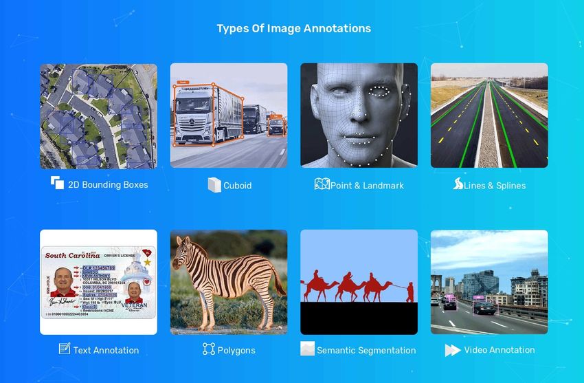
Acknowledgment

This research is the product of collective effort put in by many people and I would
take this opportunity to acknowledge their contributions. First and foremost, I would
like to thank my daily supervisor Dr. Andreas Kamilaris for all his valuable guidance,
for the time he has invested in me which has enhanced my critical thinking ability
and all the encouragement that pushed me forward to delivery my best.

    I would also like to extend my deepest gratitude to my committee Prof. Dr. Paul
Havinga and Ir. E. Molenkamp for their precious time and helping me to quickly fin-
ish my graduation process. Furthermore, I am very much indebted to Dr. Savvas
Karatsiolis (RISE, Cyprus) for his technical inputs throughout my thesis. I would also
like to remember and thank Dr. Nirvana Meratnia for organizing my thesis work in
pervasive systems group. I would like to give thanks to Jacob Kamminga for his
inputs and Pervasive System group members for making my stay during the thesis
work a comfortable one.

   Finally, I would like to acknowledge and thank Ms. Nicole Baveld for her support
and quick replies. Last but not least, I would like to express my hearty gratitude to
my parents, family, and all my friends for their unwavering faith in me and undying
support that kept me strong through the entire journey of my master program.

                                          iii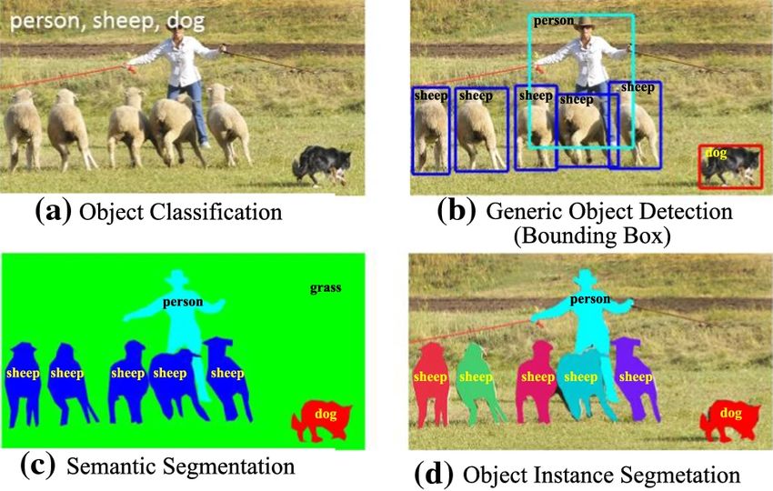

Abstract

The ability to automatically count animals may be essential for their survival. Out
of all living mammals on Earth 60% are livestock, 36% humans, and only 4% are
animals that live in the wild. In a relatively short period, human development of civi-
lization caused a loss of 83% of all wildlife and 50% of all plants. The rate of species
extinctions is accelerating. Wildlife surveys provide a population estimate and are
conducted for various reasons such as species management, biology studies, and
long term trend monitoring. In this thesis, we propose the use of deep learning
(DL), together with satellite imagery, to count the numbers of sea lions with high
precision. The proposed approach shows promising results than the state-of-art DL
models used for counting, indicating that proposed method has the potential to be
used more widely in large-scale wildlife surveying projects and initiatives.

                                           v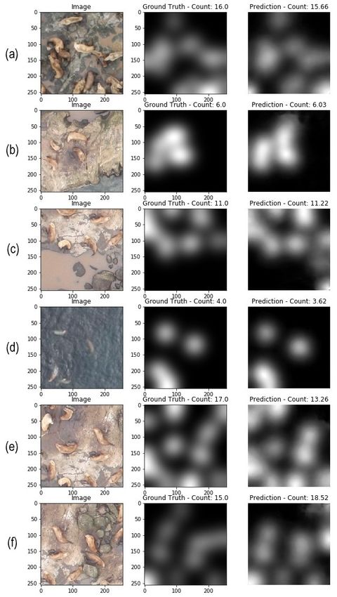
vi ABSTRACT
Contents

Acknowledgment                                                                             iii

Abstract                                                                                    v

1 Introduction                                                                              1
  1.1 Research Question . . . . . . . . . . . . . . . . . . . . . . . . . . . . . . .       2
  1.2 Thesis Outline . . . . . . . . . . . . . . . . . . . . . . . . . . . . . . . . . .    3

2 Background/Related Works                                                                  5
  2.1 Deep Learning Methods in Computer Vision . . . . . . . . . . . . . . . .              5
       2.1.1 Image Classification . . . . . . . . . . . . . . . . . . . . . . . . . .       5
       2.1.2 Object Detection and Localization . . . . . . . . . . . . . . . . . .          7
       2.1.3 Image Segmentation . . . . . . . . . . . . . . . . . . . . . . . . . . 10
       2.1.4 Image Annotation: . . . . . . . . . . . . . . . . . . . . . . . . . . . 11
       2.1.5 Counting Related Works . . . . . . . . . . . . . . . . . . . . . . . . 11
  2.2 Summary . . . . . . . . . . . . . . . . . . . . . . . . . . . . . . . . . . . . . 13

3 Dataset                                                                                  15
  3.1 Data Collection . . . . . . . . . . . . . . . . . . . . . . . . . . . . . . . . . . 15
  3.2 Data Preparation . . . . . . . . . . . . . . . . . . . . . . . . . . . . . . . . . 15
  3.3 Summary . . . . . . . . . . . . . . . . . . . . . . . . . . . . . . . . . . . . . 17

4 Methodology                                                                              19
  4.1 Overview . . . . . . . . . . . . . . . . . . . . . . . . . . . . . . . . . . . . . 19
  4.2 Density Map . . . . . . . . . . . . . . . . . . . . . . . . . . . . . . . . . . . 20
       4.2.1 Density Map Generation: . . . . . . . . . . . . . . . . . . . . . . . 21
       4.2.2 Counting from Density Map . . . . . . . . . . . . . . . . . . . . . . 22
  4.3 Model . . . . . . . . . . . . . . . . . . . . . . . . . . . . . . . . . . . . . . . 22
       4.3.1 Implementation . . . . . . . . . . . . . . . . . . . . . . . . . . . . . 23
       4.3.2 Training Parameter . . . . . . . . . . . . . . . . . . . . . . . . . . . 24
  4.4 Summary . . . . . . . . . . . . . . . . . . . . . . . . . . . . . . . . . . . . . 26

                                            vii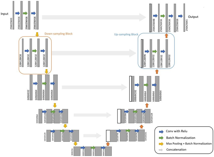
viii                                                                                                     CONTENTS

5 Performance Evaluation                                                                                                         27
  5.1 Training Results . . . . . . . . . . . . . .   .   .   .   .   .   .   .   .   .   .   .   .   .   .   .   .   .   .   .   27
  5.2 Model Evaluation . . . . . . . . . . . . . .   .   .   .   .   .   .   .   .   .   .   .   .   .   .   .   .   .   .   .   28
       5.2.1 Performance Metrics . . . . . . .       .   .   .   .   .   .   .   .   .   .   .   .   .   .   .   .   .   .   .   28
       5.2.2 Testing Results . . . . . . . . . .     .   .   .   .   .   .   .   .   .   .   .   .   .   .   .   .   .   .   .   28
  5.3 Discussion . . . . . . . . . . . . . . . . .   .   .   .   .   .   .   .   .   .   .   .   .   .   .   .   .   .   .   .   29
       5.3.1 Comparison with Model-K . . . .         .   .   .   .   .   .   .   .   .   .   .   .   .   .   .   .   .   .   .   30
       5.3.2 Comparison with Count-ception           .   .   .   .   .   .   .   .   .   .   .   .   .   .   .   .   .   .   .   30
       5.3.3 Visualization . . . . . . . . . . . .   .   .   .   .   .   .   .   .   .   .   .   .   .   .   .   .   .   .   .   31
  5.4 Summary . . . . . . . . . . . . . . . . . .    .   .   .   .   .   .   .   .   .   .   .   .   .   .   .   .   .   .   .   35

6 Conclusions                                                                            37
  6.1 Future Works . . . . . . . . . . . . . . . . . . . . . . . . . . . . . . . . . . . 37

References                                                                                                                       39
List of Figures
2.1 Simple CNN model representing image classification [1] . . . . . . . . . . . . 6
2.2 Few commonly used activation functions [2] . . . . . . . . . . . . . . . . . . 6
2.3 Alenet block diagram [3] . . . . . . . . . . . . . . . . . . . . . . . . . . . . . 7
2.4 Object detection and localization with bounding box [4] . . . . . . . . . . . . . 8
2.5 NN architecture representation for object detection and localization [5] . . . . 8
2.6 RCNN model architecture [6] . . . . . . . . . . . . . . . . . . . . . . . . . . . 9
2.7 Sample for semantic segmentation [7] . . . . . . . . . . . . . . . . . . . . . . 11
2.8 Different types of annotations used in Deep learning for image annotation [8] 12
2.9 Output of different types of Deep learning application in Computer Vision [9] . 14
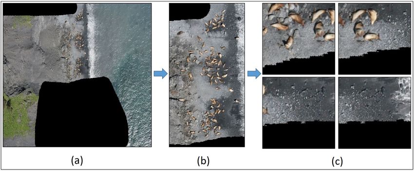
3.1 Data Preparation Workflow. (a) The original image with dimension
3328X4992. (b) Background removed image. (c) Sliding window
cropped image of dimension 256X256 . . . . . . . . . . . . . . . . . . . . 16
4.1 The proposed architecture block diagram . . . . . . . . . . . . . . . . . . 20
4.2 Training image and corresponding ground-truth Gaussian density map 22
4.3 UNet Architecture . . . . . . . . . . . . . . . . . . . . . . . . . . . . . . . . 23
4.4 Total number for parameters for Model-1 architecture . . . . . . . . . . . 24
4.5 Comparison of different classification model [10] . . . . . . . . . . . . . . 25
4.6 Total number for parameters for Model-2 architecture . . . . . . . . . . . 25
5.1 Training Loss function gradient vs. Iteration curve for Basic UNet
(Model-1) and UNet with EfficientNet-B5 feature extractor architec-
ture (Model-2) . . . . . . . . . . . . . . . . . . . . . . . . . . . . . . . . . . 27
5.2 Actual vs Predicted scatter plot . . . . . . . . . . . . . . . . . . . . . . . . 31
5.3 Actual vs Predicted density maps for Model-1 and corresponding an-
imal count for test images. From left to right: Input Image, Ground-
Truth Density Map, and Predicted Density Map . . . . . . . . . . . . . . . 32
5.4 Actual vs Predicted density maps for Model-2 and corresponding an-
imal count for test images. From left to right: Input Image, Ground-
Truth Density Map, and Predicted Density Map . . . . . . . . . . . . . . . 33
ix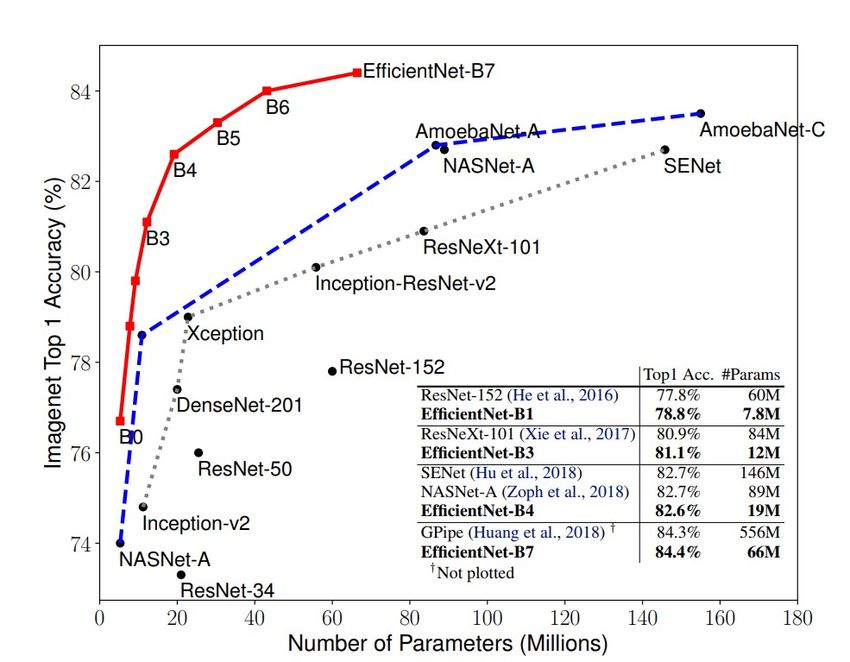
x                                                                       LIST OF FIGURES

    5.5 Test Image showing the sea lions; (a) Pups looks similar to rocks, (b)
        Pups lying very close to female sea lion . . . . . . . . . . . . . . . . . . . 34

    6.1 Circular and Ellipsoid Gaussian Density Map super imposed on Adult-
        male sea lion . . . . . . . . . . . . . . . . . . . . . . . . . . . . . . . . . . . 38
LIST OF FIGURES xi
xii LIST OF FIGURES
Acronyms

ANN Artificial Neural Network.

CCNN Count Convolutional Neural Network.

CNN Convolutional Neural Network.

GPU Graphical Processing Unit.

MAE Mean Absolute Error.

NOAA National Oceanic and Atmospheric Administration.

PCA Principal Component Analysis.

R-CNN Region-Based Convolutional Neural Network.

ReLu Rectified Linear Unit.

RMSE Root Mean Square Error.

SVM Support Vector Machine.

                                    xiii
xiv Acronyms
Chapter 1

Introduction

The ability to automatically count animals may be essential for their survival. Out
of all living mammals on Earth 60 % are livestock, 36 % humans, and only 4 % are
animals that live in the wild [11]. In a relatively short period, human development of
civilization caused a loss of 83 % of all wildlife and 50 % of all plants. Moreover, the
current rate of the global decline in wildlife populations is unprecedented in human
history – and the rate of species extinctions is accelerating [12], [13]. Wildlife sur-
veys provide a population estimate and are conducted for various reasons such as
species management, biology studies, and long term trend monitoring. This infor-
mation may be essential for species survival. For example, biologists use population
trends to investigate the effect of environmental factors such as human activity in a
region on a species’ population. This information can be used to change interna-
tional policies to benefit wildlife conservation. Using satellites or airplanes allows
biologists to survey remote species across vast areas. However, current counting
methods are laborious, expensive, and limited. Automating the counting from pho-
tographs dramatically speeds up wildlife surveys and frees up human resources for
other critical tasks. Moreover, automatic counting supports a higher frequency of
surveys to get better insights into population trends.
    NOAA Fisheries Alaska Fisheries Science Center conducts one such animal sur-
vey to count Steller sea lions’.The Steller (or northern) sea lion is the largest mem-
ber of the family Otariidae, the “eared seals”. In the 90’s Steller sea lions used to be
highly abundant throughout many parts of the coastal North Pacific Ocean. Indige-
nous peoples and settlers hunted them for their meat, fur, oil, and other products. In
the western Aleutian Islands alone, this species declined 94% in the last 30 years.
Because of this widespread population decline, Steller sea lions have been listed
as endangered species under the Endangered Species Act (ESA) in 1990 [14]. The
endangered western population of sea lions, found in the North Pacific, are the focus
of conservation efforts that require annual population counts. Having accurate pop-
ulation estimates enables us to better understand factors that may be contributing

                                           1
2 CHAPTER 1. INTRODUCTION
to a lack of recovery of Steller sea lions in this area, despite the conservation ef-
forts. Specially trained scientists at NOAA Fisheries Alaska Fisheries Science Cen-
ter conducts this survey using airplanes and unmanned aircraft systems to collect
aerial images [15]. Then trained biologists count the sea lions from the thousands of
images collected which takes up to four months for this task. Once individual counts
are conducted, the tallies are be reconciled to confirm their reliability. The results of
these counts are time-sensitive.
Automating the manual counting process will free up critical resources allowing
them to focus more on the actual conservation of sea lions. Therefore, to optimize
the counting process, the NOAA Fisheries organized a Kaggle competition dating
June 2017, seeking developers to build algorithms which accurately count the num-
ber of sea lions in aerial photographs [16].
1.1 Research Question
In this thesis, we use a novel deep learning (DL) algorithm to automatically count
Sea Lions from Aerial Images. We use the dataset from a Kaggle competition [16]
that invited participants to develop algorithms that accurately count the number of
sea lions in aerial photographs. DL is a powerful technique that has demonstrated
excellent performance for a wide range of application domains such as image pro-
cessing and data analysis [17], [18]. DL extends machine learning (ML) by adding
more "depth" (complexity) into the model, transforming the data using various func-
tions that hierarchically allow data representation, through several abstraction levels.
Compared to traditional techniques such as Support Vector Machines and Random
Forests, DL has demonstrated enhanced performance in classification and counting
computer vision-related problems [19].
This research work seeks to address the research question;
"How density map approach could be used for counting task using seg-
mentation algorithm?"
While developing a DL algorithm for automatic sea lions’ counting we also answer
the following research sub-questions:
• What are the different available counting techniques?
• What are the best counting techniques and data annotation for densely crowded
dataset?
• How do the proposed algorithm affected by a complex background environ-
ment in images?
• Where does the proposed algorithm stands with the Kaggle competition?1.2. THESIS OUTLINE 3
1.2 Thesis Outline
The thesis is organized as follows;
• Chapter 2, provides the background for Deep Learning in Computer Vision,
where we discuss the Image Classification, Object detection and Localization,
Segmentation, and related work for different counting techniques.
• In Chapter 3, we deal with dataset construction and preprocessing techniques.
• In Chapter 4, we discuss our implemented methodology.
• In Chapter 5, we evaluate the performance of the proposed algorithm.
• Finally, Chapter 6 concludes the thesis and presents a section for future work.4 CHAPTER 1. INTRODUCTION
Chapter 2

Background/Related Works

2.1       Deep Learning Methods in Computer Vision
Image classification, object detection and localization are some of the major chal-
lenges in computer vision. DL methods such as Convolutional Neural Networks
(CNN) have pushed the limits of traditional computer vision techniques to solve
these challenges. Deep learning (DL) is a branch of machine learning that uses
Artificial Neural Networks (ANN)1 with many layers. A deep neural network ana-
lyzes data with learned representations similar to the way a person would look at
a problem. Rapid progressions in DL and improvements in device capabilities in-
cluding computing power, memory capacity, power consumption, image sensor res-
olution, and optics have improved the performance and cost-effectiveness of further
quickened the spread of vision-based applications [20].

2.1.1     Image Classification
Image Classification is a systematic arrangement of images in groups and cate-
gories based on its features i.e. in simple words for a given input image, outputting
the class labels or the probability that input image is of a particular class, as shown in
Figure.2.1. Before DL, the traditional Computer Vision (CV) techniques used hand-
crafted feature extraction for classification. Features are individual measurable or
informative properties of an image. CV algorithms used edge detection, corner de-
tection or threshold segmentation algorithms to extract features. Each individual
class will have its own distinct features, based on which classification is done. The
difficulty with the CV approach is that it requires choosing which features are im-
portant in each given image for each class. As the number of classes to classify
  1 ANN  are computing systems vaguely inspired by the biological neural networks that constitute
animal brains.

                                               5
6 CHAPTER 2. BACKGROUND/RELATED WORKS
Figure 2.1: Simple CNN model representing image classification [1]
increases, feature extraction will become a more complex task.
The DL’s Convolutional Neural Network (CNN) solves this problem, it uses con-
volutional layers for feature extraction eliminating the manual feature extraction. A
typical CNN classifier architecture consist of repeated blocks of Convolutional layer
with activation function followed by max-pooling layer and finally a fully connected
layer with output Neurons matching number of class as shown in Figure.2.1.
• Convolutional layers are nothing but a set of learn-able 2D filters. Each filter
learns how to extract features and patterns present in the image. The filter is
convolved across the width and height of the input image, and a dot product
operation is computed to give an activation map.
• After each convolution operation, an Activation function is added to decide
whether that particular neuron fires or not. The activation function is a math-
ematical equation that determines the output of a neuron. There are different
activation functions with different characteristics as illustrated in Figure.2.2.
Figure 2.2: Few commonly used activation functions [2]
• Different filters that detect different features are convolved with the input image
and the activation maps are stacked together to form the input for the next2.1. DEEP LEARNING METHODS IN COMPUTER VISION 7
layer. By stacking more activation maps, we can get more abstract features.
However, as the architecture becomes deeper, we may consume too much
memory. In order to solve this problem, Pooling layers are used to reduce
the dimension of the activation maps. Pooling layers will discard a few values
either by keeping maximum value (Max Pooling) or by averaging the values
(Average Pooling). By discarding some values in each filter, the dimension of
the activation map is reduced. This means that if some features have already
been identified in the previous convolution operation, then a detailed image is
no longer needed for further processing, and it is compressed to less detailed
pictures.
• Finally, the convolution blocks is connected to Fully Connected layer which
takes the output information from convolutional networks converting into an
N-dimensional vector, where N is the number of classes, and each N value
representing the probability of being a certain class.
AlexNet, VGG, ResNet etc are few state-of-art classification architectures. These
will have 100’s of feature extraction hidden layer. Once such example architecture,
AlexNet is shown in Figure.2.3
Figure 2.3: Alenet block diagram [3]
2.1.2 Object Detection and Localization
Object detection and Localization is an automated method for locating interesting
object or multiple objects in an image with respect to the background i.e. given
an input image possibly with multiple objects, we need to generate a bounding box
around each object and classify the objects, as shown in Figure.2.4.8 CHAPTER 2. BACKGROUND/RELATED WORKS
Figure 2.4: Object detection and localization with bounding box [4]
The general idea behind object detection and Localization is to predict the prob-
ability of the object being in a class (label) along with the coordinates of the object
location. Predicting label is a classification problem and generating coordinates can
be seen as regression problem2 , which is illustrated in Figure.2.5. The total loss for
the architecture will be a combination of classification loss and regression loss.
Figure 2.5: NN architecture representation for object detection and localization [5]
Multiple object detection and localization tasks can be solved with two approaches,
which lead to two different categories of object detection algorithm.
• Two-Stage Method: This method will first perform a region proposal. This
means regions highly likely to contain an object are selected either with tradi-
tional computer vision techniques (like selective search), or by using a deep
learning-based region proposal network (RPN). Once a small set of candidate
2 Regression is a statistical approach to find the relationship between variables2.1. DEEP LEARNING METHODS IN COMPUTER VISION 9
windows is gathered, we can formulate a set of number of regression models
and classification models to solve the object detection problem. This category
includes algorithms like Faster R-CNN [21], R_FCN [22], and FPN-FRCN [23].
Algorithms in this category are usually called two-stage methods. They are
generally more accurate, but slower than the single-stage method which is
discussed below.
• Single-Stage Method: This method only looks for objects at fixed locations
with fixed sizes. These locations and sizes are strategically selected so that
most scenarios are covered. These algorithms usually separate the original
images into fixed-size grid regions. For each region, these algorithms try to
predict a fixed number of objects of certain, pre-determined shapes and sizes.
Algorithms belonging to this category are called single-stage methods. Ex-
amples of such methods include YOLO [24], SSD [25] and RetinaNet [26].
Algorithms in this category usually run faster but are less accurate. This type
of algorithm is often utilized for applications requiring real-time detection.
Example
R-CNN was one of the state-of-art object detection architecture described in [6]
(2014) by Ross Girshick, et al. from UC Berkeley. It was one of the first large
and successful application of convolutional neural networks to the problem of object
localization, detection, and segmentation. The approach had achieved then state-
of-the-art results on the VOC-2012 dataset and the 200-class ILSVRC-2013 object
detection dataset. The proposed R-CNN model is comprised of three modules;
Figure 2.6: RCNN model architecture [6]
• Module 1: Region Proposal. Extracts independent ROI from the image. A
computer vision technique is used to propose candidate regions or bounding
boxes of potential objects in the image called “selective search,” although the
flexibility of the design allows other region proposal algorithms to be used.10 CHAPTER 2. BACKGROUND/RELATED WORKS
• Module 2: Feature Extractor. Extract features from each ROI. The feature
extractor used by the model was the AlexNet. The output of the CNN was a
4,096 element vector that describes the contents of the image.
• Module 3: Classifier. Classifies features as one of the known classes. A
linear SVM for classification is used, specifically one SVM is trained for each
known class.
2.1.3 Image Segmentation
Semantic segmentation:
Semantic segmentation, or image segmentation, is the task of clustering parts of
an image together that belong to the same object class. It is a form of pixel-level
prediction i.e. image classification at the pixel level, because each pixel in an image
is classified according to a category as shown in Figure.2.7.a. Since the problem
is defined at the pixel level, determining only image class labels and location is not
acceptable, but localizing them at the original image pixel resolution is necessary.
A general semantic segmentation architecture can be broadly thought of an en-
coder network followed by an decoder network.
• The Encoder is usually a pretrained classification architecture like AlexNet,
VGG, or ResNet, which takes an input image and generates a high-dimensional
feature vector.
• Decoder, semantically projects the discriminative features (lower resolution)
learned by the encoder onto the pixel space (higher resolution) to get a dense
classification.
Semantic segmentation not only requires discrimination at pixel level but also a
mechanism to project the discriminative features learn at different stages of the en-
coder onto the pixel space.
Instance Segmentation:
Instance segmentation is a sub-type of image segmentation that identifies each in-
stance of each object within the image at the pixel level, shown in Figure.2.7.b.
Instance segmentation is an important step to achieving a comprehensive image
recognition and object detection algorithms.2.1. DEEP LEARNING METHODS IN COMPUTER VISION 11
Figure 2.7: Sample for semantic segmentation [7]
2.1.4 Image Annotation:
Image annotation is the first task in Deep learning. Image annotation is the human-
powered task of annotating an image with labels. It helps the algorithm to learn
certain patterns and store that into virtual memory to correlate or utilize the same
while analyzing similar data comes into real-life use. Bounding box, Polygon Anno-
tation, 3D Cuboid, Semantic Segmentation, Landmarking, Dot Annotation are few
types of image annotation used for different applications as illustrated in Figure.2.8.
These annotated images are used for training the model.
2.1.5 Counting Related Works
Counting objects is a challenging task for computer vision algorithms, especially
when the instance of objects varies in shape, color, or size. The state-of-art algo-
rithms has demonstrated that DL can obtain good counting performance on these
images. One of the easiest ways of counting objects using DL is first detecting the
object using CNN, and then count all found instances. This is effective but requires
bounding box annotation which is time-consuming especially when objects are heav-
ily crowded. The simplest annotation for highly crowded images is dot-annotation,
here a dot is marked on the center of each object which is used for training DL model.
So based on the annotation methods used to label the dataset, we have divided the
related works for deep-learning based counting algorithms into 3 categories;
Count via detection
In this method, a visual object detector is used to localize individual object instances
in the image. Given the localization, counting becomes trivial. In this case, objects12 CHAPTER 2. BACKGROUND/RELATED WORKS Figure 2.8: Different types of annotations used in Deep learning for image annotation [8] are annotated by a bounding box. Several methods [27], [28], [29], use this type of detection for counting objects. For instance in [27], the authors use the NOAA sea lion dataset proposing a sliding window detection and classification algorithm for counting sea lions. However, counting via detection suffer from occlusion among objects. Moreover, the annotation of densely crowed images is expensive. Count via image-level regression This way of counting is based on image-level label regression which is the least expensive annotation technique. In [30], the authors proposed a regression model for counting tomatoes, where the model learns directly from the input image and predicts the number of tomatoes in the image. Authors claim an accuracy of 91% on real images. Furthermore, the winner of the Kaggle Sealion competition [31] used an image regression method for count estimation. The methods mentioned above can only perform counting but not localization of the object. Thus, they cannot be used in cases where we are interested in both counting as well as localization of the objects.
2.2. SUMMARY                                                                     13

Count via density map

In this case, annotation involves marking a point corresponding to each object’s
location in the image from which a density heat map is generated, wchi is used for
training. The density map gives the spatial distribution of objects in a given image
relative to the total number of objects, which helps us better understand the scene
information and reduce the effect of occlusion. The Learning-to-count model of [32]
introduces a counting approach, which works by learning a linear mapping from
local image features to object density maps. By properly training the DL model, one
can estimate the object count by simply integrating over regions in the density map
produced by the model. The same strategy has also been followed in [33], [34] and
[35]. The novel model called Counting CNN (CCNN) and Hydra CNN were proposed
in [34] for counting crowd density. Essentially, the CCNN model is formulated as a
regression model where the network learns how to map the appearance of the image
patches to their corresponding object density maps. The Hydra CNN constitutes a
scale-aware counting model in order to estimate object densities in various heavily-
crowded scenarios where no geometric information of the scene can be provided.
Similarly, the authors in [35] proposed a modified CCNN model, which is a model
composed of a combination of CCNN and ResNeXt, to estimate the pig density in
pig livestock farms. [33] proposed the DisCountNet model, a two-stage network that
uses theories from both detection and density-map networks. At the first stage,
DiscNet performs a coarse detection of the patches of images from a larger input
image which has dense objects. Following this, the CountNet model operates on
the dense regions of the sparse matrix to generate a density map, which provides
fine locations and count predictions on densities of objects. Here, the author makes
a few assumptions based on observations made on the dataset. Thus, this method
needs prior information about the dataset while choosing the parameters.
    Summing up, the counting techniques mentioned above, it revolve around two
distinct characteristics of the input data:

  1. Sparse data which favors detection networks.

  2. Dense data where density map networks are used.

2.2    Summary
In this chapter we saw various types of deep learning architecture solving different
problems. Figure.2.9 demonstrate the output of classification, Object detection, Se-
mantic segmentation, and Object Instance Segmentation method on a given input
image.
14 CHAPTER 2. BACKGROUND/RELATED WORKS
Figure 2.9: Output of different types of Deep learning application in Computer Vision [9]
In this thesis work, our solution treat sea lion counting problem as counting via
density map. The proposed model uses semantic segmentation algorithms for den-
sity estimation without pixel-level annotation. We use dot annotation i.e. placing
dots at the center of each animal and then generate a Gaussian density map from it,
this largely reduces annotation overhead. The proposed solution greatly improves
the counting and localization performance with minimum annotation.Chapter 3
Dataset
3.1 Data Collection
The Steller Sea Lion dataset from NOAA fisheries [16], consists of 948 aerial im-
ages, which have different categories of sea lions based on age and gender of the
animals: adult males (also known as bulls); sub-adult males; adult females; juve-
niles; and pups. For each image, there are two versions: the original image as well
as the one with dots in the center of each sea lion. Image resolution was not uniform
but was roughly around 5000X 3000, each image roughly occupying around 5MB. The
dataset was split into training (0-800) and testing images (801-947) with 85:15 ratio
respectively. The testing images were used for assessing the model’s performance.
During this phase, the following observations were made on the dataset:
1. The large image resolution gave better details (Figure.3.1.a), but required large
memory size(RAM).
2. The number of sea lions per images varied widely between 3 and 900 animals
3. In most of the images, the sea lions were gathered together in the same place,
leaving large portions of the image with only background
3.2 Data Preparation
To address the observations and challenges described in previous Section, we per-
formed few image pre-processing methods which is illustrated in Figure.3.1.
• First, we used rough cropping to remove the portion of image which had only
background, refer Figure.3.1b.
1516 CHAPTER 3. DATASET
• We set the input image size to 256X 256. Instead of resizing the original image,
we used sliding window cropping with roughly 10% overlap. Approximately,
180000 images of resolution 256X 256 was generated, refer Figure.3.1c
• Post cropping we noticed that few of the images did not had any Sea lions
in it, an example is shown in Figure.3.1c crop 3 and 4. These images were
discarded.
Figure 3.1: Data Preparation Workflow. (a) The original image with dimension
3328X4992. (b) Background removed image. (c) Sliding window
cropped image of dimension 256X256
For the new training images with size 256X 256, the number of sea lion per image
ranged from 1-80 with mean 4 and standard deviation 6. Table 3.1 shows the sea
lions’ distribution in the training dataset. Further, for training the train dataset was
split into Train and Valid set with 80:20 ratio.
Table 3.1: Training images sea lions distribution per image
Sea lions per image Total no. of images
01 - 20 54,870
21 - 40 1,468
>40 1273.3. SUMMARY 17
3.3 Summary
This chapter focused on Dataset used for our work. We discussed our observation
on the dataset and propose the data preparation method. Post data preparation we
were able to get 56465 Training images and 2842 testing image (Table 3.2).
Table 3.2: Training (Train+Valid) and Testing dataset split
Dataset No.of Images
Training Images (Train+Val) 56465
Testing Images 284218 CHAPTER 3. DATASET
Chapter 4

Methodology

4.1    Overview
As discussed earlier, to estimate the number of objects in an image, there are gen-
erally three methods. One is to input the image, use an object detection algorithm to
detect the object instances, and then count instance. Second, is to input the image,
regress the input image and output the total count. And the last one is to input the
image, predict the distribution density map, and get the number of object by sum-
ming the density distribution. Our solution treats the counting problem as the third
one, an object density estimation task. The reasons are as follows:

   • In general, the count via detection and count via regression are not accurate
     enough, and struggles especially when the objects are at different perspec-
     tives, different postures, and highly occluded.

   • For example, count via regression directly gives the object count without having
     any distribution detail or scene information which makes it difficult to visualize
     the result. In count via detection a large number of candidate windows need to
     be detected during the detection process, which reduces the efficiency of the
     algorithm and is not suitable for scenes with multi-perspective and multi-object
     overlapping.

   • The proposed density map approach gives the spatial distribution of objects
     in a given image relative to the total number of objects, which helps us to
     better understand the scene information. The object count can be counted by
     spatial integration, and local area analysis can be performed to produce more
     accurate numbers.

   • Counting via density map is also more suitable for images with different per-
     spective and occlusion.

                                         19
20 CHAPTER 4. METHODOLOGY
Considering this an end-to-end model was designed that takes an input image
and produces a density map with the precise localization of the animal. To gener-
ate density map a semantic segmentation model, UNet [36] is proposed.The main
disadvantage of semantic segmentation algorithms is the tedious pixel-level annota-
tion. Our solution uses dot annotation, which largely reduces annotation overhead.
The proposed solution greatly improves the counting and localization performance
with minimum annotation.
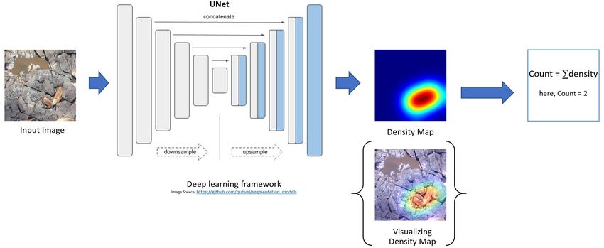
An illustration of the proposed solution is shown in Fig.4.1. The input image is
fed to the proposed architecture, the Encoder section of the architecture generates a
high dimensional feature vector. Decoder, semantically projects the feature learned
by the encoder onto the pixel space generating corresponding density distribution
for the given image. This density map is used to get the number of objects by simply
integrating the density distribution over the region.
Figure 4.1: The proposed architecture block diagram
4.2 Density Map
In order to estimate the object count in an image, the model needs to learn from the
density distribution of the individual image, and once the model learns to generate
density distribution we need to calculate the total count from it. In this section we will
formalize mathematical definition to generate a ground-truth density map and how
we can arrive at the object count from predicted density map.4.2. DENSITY MAP 21
Table 4.1: Average size of Sea-lion based on their classes
Class Size(Avg)
adult males 80X60
sub-adult males 70X40
adult females 60X40
juveniles 40X30
pups 30X20
4.2.1 Density Map Generation:
The Kaggle dataset consisted of sea lion images along with its corresponding dot
annotated images. This dot annotation was done by expert NOAA biologists. The
dotted images were used to extract the coordinates of the center of each sea lions
which is used to generate the ground-truth density map. The density map is gen-
erated by processing the center of point objects with a Gaussian smoothing kernel,
Figure.4.2.
For the given set of annotated images, where all the animals have been marked
with dots, the ground truth density map D I , for an image I, is defined as a sum of
Gaussian functions centered at each dot annotation.
N (p; µ, ), (4.1)
X P
D I (p) =
µ∈A I
where A I is the set of 2D points annotation for image I and N (p; µ, ) represents an
P
isotropic 2D Gaussian function, with a mean µ and a covariance matrix , evaluated
P
at pixel position p . Covariance =σ2 I is a diagonal matrix with σ controlling the
P
spread of the distribution. Based on the average size of the sea lion, we chose
σ = 5.
When 2 points intersects the density map of this intersection area is superim-
posed. Hence, the density map approach is suitable for problems with sparsely
distributed objects as well as images with occlusion, overlapping, and varied per-
spectives.22 CHAPTER 4. METHODOLOGY
Figure 4.2: Training image and corresponding ground-truth Gaussian density map
4.2.2 Counting from Density Map
The density map provides the spatial distribution of objects in a given image, relative
to the total number of objects. Given the density map, D I the total count N I can be
obtained by integrating the pixel values in density map D I over the entire image as
below:
(4.2)
X
NI = D I (p)
p∈I
4.3 Model
The feed-forward regression networks in [34], [35] compress and encode images
into smaller representation vectors. The combination of CCNN+ResNeXt model
in [35] takes an input image of size 72X 72 and produces an output density map
of size 18X 18. Due to down-sampling and the loss of spatial resolution in higher
layers, there is a possibility to lose information. To avoid this, an encoder-decoder
architecture, named UNet is proposed as a learning architecture.
UNet is a Convolutional Neural Network (CNN) architecture, proposed in [36]
for biomedical image segmentation. UNet is an encoder-decoder-type network ar-
chitecture for image segmentation. The name of the architecture comes from its
distinct shape, where the feature maps from the down-sampling block are fed into
the up-sampling block. The down-sampling path captures context and a symmetric
up-sampling path enables precise localization.
Figure 4.3 shows the architecture of the UNet, where each gray box corresponds
to a multi-channel feature map. Yellow box represents the downsampling block and
the Blue box represents the Up-sampling block. The size and number of channels4.3. MODEL 23
Figure 4.3: UNet Architecture
[x,y,c] is provided at the lower-left edge of the box. White boxes represent copied
feature maps. The arrows denote the different operations.
The Down-sampling/Contracting path consists of the repeated application of two
3X 3 convolutions, each followed by a ReLU, batch-normalization layer, and a 2X 2
max pooling operation with stride 1. The number of feature channels (filter size) is
doubled at each downsample block.
Similarly, the Up-sampling/Expansive path consists of a 2X 2 2D up-sampling
convolution with the nearest interpolation. The up-sampling of the feature maps
halves the number of feature channels. This is concatenated with the correspond-
ingly cropped feature map from the contracting path, which is followed with two 3X 3
convolutions, with ReLU activation. At the final layer, a 1X 1 convolution is used to
map feature vector to the desired number of classes. The input data is normalized
before feeding it into the network.
4.3.1 Implementation
To verify the effectiveness of the proposed network architecture, two models were
trained:24 CHAPTER 4. METHODOLOGY
Model-1
Model-1 is the basic UNet without any existing feature extractor architecture. The
UNet architecture shown in figure 4.3 was implemented in Keras using a Tensorflow
backend. The model have 5 downsampling block and 5 upsampling block. The
figure 4.4 shows the total number of parameters for the implemented model.
Figure 4.4: Total number for parameters for Model-1 architecture
Model-2
Here an existing classification model with pre-trained weights is used as feature ex-
traction. Resnet, Resnext, VGG19, Inceptionv3, densenet, inceptionresnetv2, mo-
bilenet, efficientnetb are few state-of-art classification models that could be used
as a feature extractor. Figure 4.5 show the comparison between different architec-
tures. For our application we use Efficientnet version-’5’ [10] as a feature extrac-
tor. Effiecientnet is a Convolutional Neural Network developed by google, that has
set new records for both accuracy and computational efficiency. In high-accuracy
regime, with 66M parameters and 37B FLOPS. At the same time, the model is 8.4x
smaller and 6.1x faster on CPU inference than the former leader, Gpipe.
The architecture was implemented on Keras using TensorFlow backend [37]. Ef-
ficientNetB5 is used as a feature extractor to build the UNet model. All the layer was
set as trainable. ’BatchNormalization’ layer was used between the 2D-Convolution
layer and activation. As we have only one class i.e. sea-lion class, the output ac-
tivation was set to ’sigmoid’ function instead of softmax. The model was initialized
with ’Imagenet’ pretrained weight. The figure 4.6 shows the summary of the model
parameters.
4.3.2 Training Parameter
Loss Function:
To make model learn, an objective optimization function is defined, which measures
the Root Mean Square Error(RMSE) between the predicted density map (D̂ ) and the4.3. MODEL 25
Figure 4.5: Comparison of different classification model [10]
Figure 4.6: Total number for parameters for Model-2 architecture
true density map (D ), defined as:
v
N
u
u1 X
L=t (D̂ − D)2 (4.3)
N n=1
Optimizer:
All the parameters were optimized using Adam with a learning rate of 0.001. A
learning rate reduction during training was also used for further improvement. The
Nvidia GeForce RTX 2060 GPU was used for training, with a batch size of 8.26 CHAPTER 4. METHODOLOGY 4.4 Summary In this chapter we discussed the overview of the proposed architecture. We defined mathematical formulas for Gaussian based counting approach. The architecture description and their implementation details were mentioned. Finally the parameters used for the training the model was stated.
Chapter 5

Performance Evaluation

5.1    Training Results
Both models were trained for 100 epochs and their training results were logged.
Basic UNet (Model-1) took 7 hours for training while UNet with the EfficientNet-B5
feature extractor (Model-2) took 17 hours. According to their performance on the
validation dataset, early stopping was used for selecting the model with the best
performance. Figure 5.1 shows the loss function gradient descent during training
for Model-1 and Model-2. We can see that the Model-2 which used the ’Imagenet’
pre-trained weights already having some prior information about the sea lions, con-
verged faster than Model-1. Even though the plot shows that the loss converges
to some small value for both models, the Model-2 was a little better in finding its
minima.

Figure 5.1: Training Loss function gradient vs. Iteration curve for Basic UNet
            (Model-1) and UNet with EfficientNet-B5 feature extractor architecture
            (Model-2)

                                        27
28 CHAPTER 5. PERFORMANCE EVALUATION
5.2 Model Evaluation
5.2.1 Performance Metrics
For performance evaluation of the proposed models, we use Mean Absolute Error
(MAE) and Root Mean Square Error (RMSE) to measure the accuracy of the pre-
dicted count.
Mean Absolute Error:
MAE is the average of the absolute differences between predicted and actual count.
It measures the average magnitude of the errors in a set of predictions.
1 X N
M AE = |(y i − yˆi )| (5.1)
N i =1
where y i is the actual sea lion count in the i th image, yˆi is the predicted sea lion
count in the i th image and N is the total number of test images.
Root Mean Square Error:
RMSE is the square root of the average of squared differences between predicted
and actual count. Since the errors are squared before they are averaged, the RMSE
gives a relatively high weight to large errors.
v
N
u
u1 X
R M SE = t (y i − yˆi )2 . (5.2)
N i =1
where y i is the actual sea lion count in the i th image, yˆi is the predicted sea lion
count in the i th image and N is the total number of test images.
The MAE characterizes the accuracy of the algorithm, while the RMSE represents
the degree of dispersion in the differences, and examines the robustness of the
models.
5.2.2 Testing Results
The trained model was tested on the testing dataset and RMSE & MAE for animal
count is recorded.5.3. DISCUSSION 29
Table 5.1: Comparison table for Model-1 and Model-2
Model RMS(Train) MAE(Train) RMS(Test) MAE(Test) Parameters Time(min)
Model-1 1.35 0.84 3.33 1.90 ≈15M 4.27
Model-2 1.24 0.61 1.88 1.09 ≈37M 9.83
Model-1
The Model-1 with just 5 blocks (downsampling and upsampling) having only 15M
parameters was able to achieve a reasonably good result. The model reached an
RMSE and MAE value of 1.35 & 0.84 respectively for training images and 3.33 &
1.90 respectively for test images (Table 5.1). Figure 5.3 shows a few test image
predicted density maps, its corresponding ground-truth density map, and the animal
counts for Model-1.
Model-2
The Model-2 with efficientnet as a feature extractor having 37M parameters out-
performed the Model-1 with an RMSE and MAE of 1.24 and 0.61 respectively on
training images and 1.88 and 1.09 respectively on test images (Table 5.1). Figure
5.3 shows a few output prediction and corresponding ground-truth for test images.
Table 5.1 show the comparison between Model-1 and Model-2. The average RMSE
and MAE for training and test dataset and training time per epoch are given in the
table.
5.3 Discussion
To verify the effectiveness of our proposed network architecture, we compare our
solution with the Kaggle competition winning model (named Model-K from now on)
[31] and Count-ception [38], a redundant counting approach based on Inception
modules and fully convolutional network. In this section, we consider only our best-
performing model, which is Model-2. Table 5.2 shows a comparison of RMSE and
MAE for actual and predicted count between the Model-2, Model-K, and Count-
ception.30 CHAPTER 5. PERFORMANCE EVALUATION
Table 5.2: Comparison between Model-2, Model-K, and Count-ception
Model Feature Extractor RMSE MAE Parameters
Model-2 Eff.Net-B5 1.88 1.09 ≈37M
Model-K VGG 2.17 1.43 ≈48M
Count-ception No 5.57 3.54 ≈14M
5.3.1 Comparison with Model-K
The Kaggle winning model (Model-K) [31] architecture is a regression model with
VGG16 without top as a feature extractor. The output layer was flattened and given
to 2 FC layers with linear output. Model-K was initialized with pre-trained Imagenet
weights and then trained using our training dataset. The model was trained using
an Stochastic Gradient Descent (SGD) optimizer and an Mean Square Error (MSE)
loss function. The trained model was tested with a test dataset and the results are
tabulated in Table 5.2.
The Model-K with 48M parameter was able to reach an RMSE and MAE of 2.17
and 1.43 respectively, but our proposed Model-2 with efficientnet feature extractor
having 37M parameters gave slightly better results with RMSE and MAE of 1.88
and 1.09 respectively. Our model gave better counting accuracy with lesser model
complexity.
5.3.2 Comparison with Count-ception
Count-ception network [38] use Inception modules to build a network targeting at
counting object in the image. The whole network is a fully convolutional neural net.
In order not to lose pixel information, no pooling layer is used in the architecture.
After each convolution, batch normalization and leaky ReLU activation are used to
speed up convergence. The model implementation was directly taken from [39]. The
model takes an input image and predicts a map. The count from the prediction can
be calculated using the below formula;
P
x,y F (I )
count = (5.3)
r2
where F(I) is predicted map and r is receptive field size (here, 32) The model was
trained and tested with our dataset. For test images the model gave an RMSE and
MAE value of 5.85 and 3.81 respectively (Table 5.2). The model had better counting
accuracy for images with less overlap, but the accuracy largely dropped when the
overlap was high and the sea lions’ lay close to the image boundary. In our proposed5.3. DISCUSSION 31
(a) Model-1 (b) Model-2
Figure 5.2: Actual vs Predicted scatter plot
Gaussian density approach, it treats the object lying close to the boundary as a
fraction but Count-ception fails to do it resulting in a decrease in count accuracy.
5.3.3 Visualization
Actual vs Predict Count
To visualize the accuracy of predicted count of proposed Model-2 for test images, we
plot an actual vs prediction count scatter plot for both models, as shown in Figure
5.2. The diagonal red line represents the zero error, closer the points to the line
better the prediction. The plots show that Model-2 with efficientnet feature extractor
has a better prediction result compared to Model-1.
Model Outputs
Figure 5.3 and Figure 5.4 show a few test images together with their actual and
predicted density maps and the animal count, for Model-1 and Model-2 respectively.
The Figure 5.3,5.4 (images [a-d]) shows few example predcition where the difference
between the actual and predicted count is small. Both the models are not heavily af-
fected by different illumination, occlusion, and overlapping. The models were able to
perform well despite the challenging environmental conditions like under-water and
complex background. Figure 5.3, 5.4 (image [e-f]) show examples of a noticeable
difference between the true count and predicted count. The major contribution for
the error was from juveniles and pups in the images, this is mainly because;
• Juveniles and pups are inherently difficult to be detected because of their
smaller size compared to other sea lion types. The pups look like rocks in
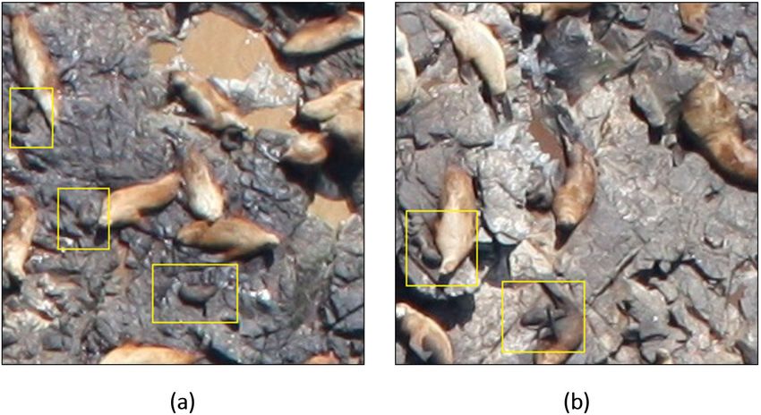
the background 5.5(a).32 CHAPTER 5. PERFORMANCE EVALUATION
Figure 5.3: Actual vs Predicted density maps for Model-1 and corresponding animal
count for test images. From left to right: Input Image, Ground-Truth
Density Map, and Predicted Density Map5.3. DISCUSSION 33
Figure 5.4: Actual vs Predicted density maps for Model-2 and corresponding animal
count for test images. From left to right: Input Image, Ground-Truth
Density Map, and Predicted Density Map34 CHAPTER 5. PERFORMANCE EVALUATION
Figure 5.5: Test Image showing the sea lions; (a) Pups looks similar to rocks, (b)
Pups lying very close to female sea lion
• The pups usually tend to be closer to female sea lions (possibly their moth-
ers), appearing as part of female sea lions, a fact that makes them hard to be
detected, due to occlusion 5.5(b).5.4. SUMMARY 35 5.4 Summary In this chapter, we carry out the performance evaluation of our proposed models. First, we discuss the training results of our models. Later, we define performance metrics and evaluate & compare the models based on defined performance metrics. To know where we stand, we also compare our results with 2 other models (Kag- gle winning model and Count-ception). Finally, we visualize the model outputs and discuss the result.
36 CHAPTER 5. PERFORMANCE EVALUATION
Chapter 6

Conclusions

Multi-object counting in crowded images is an extremely time-consuming task in
real-world application. In a lot of situations, we do not need to detect each ob-
ject, which means we could avoid the hard problem of detecting individual object
instances. Considering this, in this thesis work, we present a solution for sea lion
counting from aerial images using deep learning and density map. A semantic seg-
mentation algorithm, UNet has been employed for counting task. We utilize the
advantages of the Gaussian density map for counting. The tedious pixel-level anno-
tation required for semantic segmentation algorithm is replaced with dot annotation
largely reducing annotation overhead.
    The results showed that by using EfficientNet as a feature extractor architecture,
an RMSE of 1.88 was achieved, regardless of the complex background, the differ-
ent illumination conditions, and the heavy overlapping and occlusion. The proposed
solution had a good count prediction with lesser training parameters and minimum
annotation. The main error in counting accuracy occurs due to animals’ occlusion
and small animals (especially, pups) that look like beach rocks. The proposed solu-
tion could be extended for counting other wild animals and endangered species as
this work provides general implementation rather than specific hand-crafted tech-
niques.

6.1     Future Works

During the course of this thesis work we faced few challenges which could not be
addressed fully. Also, there are few ideas which couldn’t be implemented due to
time limitations and we leave them as possible future improvements.

                                         37
38 CHAPTER 6. CONCLUSIONS
Ellipsoid Gaussian Density
For this work, we use a circular Gaussian density map as ground-truth (6.1a) even
though the density map approach can handle occlusion problems, but when animals
are heavily occluded the density map of one animals overlap with other reducing
the ability of the model to learn. So having an ellipsoid density map (6.1b) would
eliminate the density map pixel overlapping issue. But there rise one more challenge
to find the right orientation (i.e. covariance matrix), which could be done by adding
one more model to find the alignment of the sea lion.
Figure 6.1: Circular and Ellipsoid Gaussian Density Map super imposed on Adult-
male sea lion
Synthetic Dataset
Another approach to increase the prediction accuracy would be with the help of a
synthetic dataset. Synthetic data is a dataset that is artificially manufactured rather
than generated by real-world events. So by training the model with additional syn-
thetic data might help to improve the detection accuracy.
Class-wise Counting
Presently, we just concentrate on estimating the animal density from the image. In
the future, we could also focus on class-wise sea lion counting i.e. we estimate the
density map and classify each density to 5 different sea lion classes (Adult male,
Sub-adult male, Adult female, Juveniles and Pups) and get class-wise animal count.Bibliography
[1] “Simple cnn classifier model.” [Online]. Available: https:
//developers.google.com/machine-learning/practica/image-classification/
images/cnn_architecture.svg
[2] “Activation function.” [Online]. Available: https://miro.medium.com/max/1200/
1*ZafDv3VUm60Eh10OeJu1vw.png
[3] “Alexnet block diagram.” [Online]. Available: https://missinglink.ai/wp-content/
uploads/2019/08/AlexNet-2012.png
[4] “Object detection image.” [Online]. Available: https://www.arunponnusamy.
com/images/yolo-object-detection-opencv-python/yolo-object-detection.jpg
[5] “Object detection block diagram.” [Online]. Available: https://miro.medium.com/
max/1400/1*NTVoRZYBWbwRxNidyLCxPw.png
[6] R. B. Girshick, J. Donahue, T. Darrell, and J. Malik, “Rich feature hierarchies
for accurate object detection and semantic segmentation,” CoRR, vol.
abs/1311.2524, 2013. [Online]. Available: http://arxiv.org/abs/1311.2524
[7] “Image segmentation.” [Online]. Available: https://miro.medium.com/max/2436/
0*QeOs5RvXlkbDkLOy.png
[8] “Image annotation.” [Online]. Available: https://miro.medium.com/max/1400/
1*-mnmd7hI1mEAoQBsrRMpLA.jpeg
[9] “Deep learning summary.” [Online]. Available: https://glassboxmedicine.files.
wordpress.com/2020/01/coco-task-examples-1.png?w=616
[10] M. Tan and Q. V. Le, “Efficientnet: Rethinking model scaling for convolutional
neural networks,” CoRR, vol. abs/1905.11946, 2019. [Online]. Available:
http://arxiv.org/abs/1905.11946
[11] Y. M. Bar-On, R. Phillips, and R. Milo, “The biomass distribution on Earth,”
Proceedings of the National Academy of Sciences, vol. 115, no. 25, pp. 6506–
6511, jun 2018. [Online]. Available: https://www.pnas.org/content/115/25/6506
3940 BIBLIOGRAPHY
[12] S. Diaz, J. Settele, E. Brondizio, H. T. Ngo, M. Gueze, J. Agard, A. Arneth,
P. Balvanera, K. Brauman, S. Butchart, K. Chan, L. Garibaldi, K. Ichii, J. Liu,
S. M. Subramanian, G. Midgley, P. Miloslavich, Z. Molnar, D. Obura, A. Pfaff,
S. Polasky, A. Purvis, J. Razzaque, B. Reyers, R. R. Chowdhury, Y.-J. Shin,
I. Visseren-Hamakers, K. Willis, and C. Zayas, “Summary for policymakers of
the global assessment report on biodiversity and ecosystem services,” Tech.
Rep. May 2019, 2019. [Online]. Available: https://www.ipbes.net/news/ipbes/
ipbes-global-assessment-summary-policymakers-pdf
[13] J. Kamminga, E. Ayele, N. Meratnia, and P. Havinga, “Poaching detection
technologies-A survey,” Sensors (Switzerland), vol. 18, no. 5, p. 1474, 2018.
[14] U.S. Fish and Wildlife Service, “Endangered species act,” 1973,
https://www.fisheries.noaa.gov/topic/laws-policies#endangered-species-act.
[15] N. F. A. F. S. Cente, “Noaa fisheries steller sea lion survey reports.” [Online].
Available: https://www.fisheries.noaa.gov/alaska/marine-mammal-protection/
steller-sea-lion-survey-reports
[16] N. F. A. F. S. Center, “Noaa fisheries steller sea lion
population count.” [Online]. Available: https://www.kaggle.com/c/
noaa-fisheries-steller-sea-lion-population-count/overview
[17] J. Schmidhuber, “Deep learning in neural networks: An overview,”
Neural Networks, vol. 61, p. 85–117, Jan 2015. [Online]. Available:
http://dx.doi.org/10.1016/j.neunet.2014.09.003
[18] Y. Lecun, Y. Bengio, and G. Hinton, “Deep learning,” Nature, vol. 521, no. 7553,
pp. 436–444, 2015.
[19] A. Kamilaris and F. X. Prenafeta-Boldu, “Deep learning in agriculture:
A survey,” CoRR, vol. abs/1807.11809, 2018. [Online]. Available: http:
//arxiv.org/abs/1807.11809
[20] J. Walsh, N. O’ Mahony, S. Campbell, A. Carvalho, L. Krpalkova, G. Velasco-
Hernandez, S. Harapanahalli, and D. Riordan, “Deep learning vs. traditional
computer vision,” 04 2019.
[21] S. Ren, K. He, R. Girshick, and J. Sun, “Faster r-cnn: Towards real-time object
detection with region proposal networks,” IEEE Transactions on Pattern Analy-
sis and Machine Intelligence, vol. 39, no. 6, pp. 1137–1149, 2017.You can also read