Estimation of oceanic subsurface mixing under a severe cyclonic storm using a coupled atmosphere-ocean-wave model - Ocean Science
←
→
Page content transcription
If your browser does not render page correctly, please read the page content below
Ocean Sci., 14, 259–272, 2018
https://doi.org/10.5194/os-14-259-2018
© Author(s) 2018. This work is distributed under
the Creative Commons Attribution 4.0 License.

Estimation of oceanic subsurface mixing under a severe cyclonic
storm using a coupled atmosphere–ocean–wave model
Kumar Ravi Prakash, Tanuja Nigam, and Vimlesh Pant
Centre for Atmospheric Sciences, Indian Institute of Technology Delhi, New Delhi-110016, India

Correspondence: Vimlesh Pant (vimlesh@iitd.ac.in)

Received: 5 October 2017 – Discussion started: 10 October 2017
Revised: 27 January 2018 – Accepted: 7 March 2018 – Published: 3 April 2018

Abstract. A coupled atmosphere–ocean–wave model was               1   Introduction
used to examine mixing in the upper-oceanic layers under
the influence of a very severe cyclonic storm Phailin over the    The Bay of Bengal (BoB), a semi-enclosed basin in the
Bay of Bengal (BoB) during 10–14 October 2013. The cou-           northeastern Indian Ocean, consists of surplus near-surface
pled model was found to improve the sea surface temperature       fresh water due to large precipitation and runoff from the
over the uncoupled model. Model simulations highlight the         major river systems of the Indian subcontinent (Varkey et
prominent role of cyclone-induced near-inertial oscillations      al., 1996; Rao and Sivakumar, 2003; Pant et al., 2015). The
in subsurface mixing up to the thermocline depth. The iner-       presence of fresh water leads to salt-stratified upper-ocean
tial mixing introduced by the cyclone played a central role       water column and the formation of a barrier layer (BL), a
in the deepening of the thermocline and mixed layer depth         layer sandwiched between the bottom of the mixed layer
by 40 and 15 m, respectively. For the first time over the BoB,    (ML) and the top of the thermocline, in the BoB (Lukas and
a detailed analysis of inertial oscillation kinetic energy gen-   Lindstrom, 1991; Vinayachandran et al., 2002; Thadathil et
eration, propagation, and dissipation was carried out using       al., 2007). The BL restricts the entrainment of colder wa-
an atmosphere–ocean–wave coupled model during a cyclone.          ters from thermocline region into the mixed layer; it thereby
A quantitative estimate of kinetic energy in the oceanic wa-      maintains a warmer ML and sea surface temperature (SST).
ter column, its propagation, and its dissipation mechanisms       The warmer SST together with higher tropical cyclone heat
were explained using the coupled atmosphere–ocean–wave            potential (TCHP) makes the BoB one of the active regions for
model. The large shear generated by the inertial oscillations     cyclogenesis (Suzana et al., 2007; Yanase et al., 2012; Vissa
was found to overcome the stratification and initiate mixing      et al., 2013). The majority of tropical cyclones are gener-
at the base of the mixed layer. Greater mixing was found at       ated during the pre-monsoon (April–May) and post-monsoon
the depths where the eddy kinetic diffusivity was large. The      (October–November) seasons (Alam et al., 2003; Longshore,
baroclinic current, holding a larger fraction of kinetic energy   2008). The number of cyclones and their intensity is highly
than the barotropic current, weakened rapidly after the pas-      variable on seasonal and interannual timescales. The oceanic
sage of the cyclone. The shear induced by inertial oscillations   response to the tropical cyclone depends on the stratification
was found to decrease rapidly with increasing depth below         of the ocean. The BL formation in the BoB is associated with
the thermocline. The dampening of the mixing process below        the strong stratification due to the peak discharge from rivers
the thermocline was explained through the enhanced dissipa-       in the post-monsoon season. The intensity of the cyclone
tion rate of turbulent kinetic energy upon approaching the        largely depends on the degree of stratification (Neetu et al.,
thermocline layer. The wave–current interaction and nonlin-       2012; Li et al., 2013). The coupled atmosphere–ocean model
ear wave–wave interaction were found to affect the process        was found to improve the intensity of cyclonic storms when
of downward mixing and cause the dissipation of inertial os-      compared to the uncoupled model over different oceanic re-
cillations.                                                       gions (Warner et al., 2010; Zambon et al., 2014; Srinivas et
                                                                  al., 2016; Wu et al., 2016). Zambon et al. (2014) compared
                                                                  the simulations from the coupled atmosphere–ocean and un-

Published by Copernicus Publications on behalf of the European Geosciences Union.
260                          K. R. Prakash et al.: Estimation of oceanic subsurface mixing under a severe cyclonic storm

coupled models and reported significant improvement in the         The NIO is found to decline with decreasing depth and van-
intensity of storms in the coupled case as compared to the         ishes in the coastal regions (Schahinger, 1988; Chen et al.,
uncoupled case. The uncoupled atmospheric model produced           2017).
large ocean–atmosphere enthalpy fluxes and stronger winds             The aim of this paper is to understand and quantify the
in the cyclone (Srinivas et al., 2016). When the atmospheric       near-inertial mixing due to the very severe cyclonic storm
Weather Research and Forecasting (WRF) model interacted            Phailin in the BoB. Phailin developed over the BoB in the
with the ocean model, the SST was found to be more real-           northern Indian Ocean in October 2013. The landfall of
istic compared to the stand-alone WRF (Warner et al., 2010;        Phailin occurred on 12 October 2013 around 17:00 GMT
Gröger et al., 2015; Jeworek et al., 2017; Ho-Hagemann et          near the Gopalpur district of Odisha state on the east coast
al., 2017). Wu et al. (2016) demonstrated the advantage of         of India. After the 1999 super cyclonic event of the Odisha
using a coupled model over the uncoupled model in a better         coast, Phailin was the second strongest cyclonic event that
simulation of typhoon Megi’s intensity.                            made landfall on the east coast of India (Sanil Kumar and
   Mixing in the water column has an important role in en-         Nair, 2015). The low-pressure system developed in the north
ergy and material transference. Mixing in the ocean can be         of the Andaman Sea on 7 October 2013 and was trans-
introduced by the different agents such as wind, current, tide,    formed into a depression on 8 October at 12◦ N, 96◦ E. This
eddy, and cyclone. Mixing due to tropical cyclones is mostly       depression was converted into a cyclonic disturbance on 9
limited to the upper ocean, but the cyclone-induced internal       October and further intensified while moving to the east-
waves can affect the subsurface mixing. Several studies have       central BoB, showing a maximum wind speed of 200 km h−1
observed that the mixing in the upper-oceanic layer is in-         at 03:00 GMT on 11 October. Finally, landfall occurred at
troduced due to the generation of near-inertial oscillations       17:00 GMT on 12 October. More details on the development
(NIOs) during the passage of tropical cyclones (Gonella,           and propagation of Phailin can be found in the literature
1971; Shay et al., 1989; Johanston et al., 2016). This mixing      (IMD Report, 2013; Mandal et al., 2015). The performance
is responsible for the deepening of the ML and the shoaling        of the coupled atmosphere–ocean model in simulating the
of the thermocline (Gill, 1984). The vertical mixing caused        oceanic parameters temperature, salinity, and currents during
by storm-induced NIO has a significant impact on upper-            Phailin is discussed in Prakash and Pant (2017).
ocean variability (Price, 1981). The NIO are also found to be         Most of the past studies on oceanic mixing under cy-
responsible for the decrease in SST along the cyclone track        clonic conditions were carried out using in situ measure-
(Chang and Anthes, 1979; Leipper, 1967; Shay et al., 1992,         ments, which are constrained by their spatial and temporal
2000). This decrease in SST is caused by the entrainment of        availability. To the best of our knowledge, the present study
cool subsurface thermocline water from the mixed layer into        is the first of its kind to utilize a coupled atmosphere–ocean–
the immediate overlying layer of water. This cooling of sur-       wave model over the BoB to estimate cyclone-induced mix-
face water is one of the reasons for the decay of cyclones         ing, its associated energy propagation on the cyclone track,
(Cione and Uhlhorn, 2003). The magnitude of surface cool-          and the location of maximum surface wind stress during the
ing differs largely depending on the degree of stratification      period of the peak intensity of the cyclone. The study also
on the right-hand side of the cyclone track (Jacob and Shay,       focuses on analyzing the subsurface distribution of NIO with
2003; Price, 1981).                                                its vertical mixing potential. Further, the study quantifies the
   The near-inertial process can be analyzed from the baro-        shear-generated mixing and the kinetic energy of the baro-
clinic component of currents. The vertical shear of horizon-       clinic mode of the horizontal current varying in the vertical
tal baroclinic velocities that is interrelated with buoyancy os-   section at a selected location during the active period of the
cillations of surface layers is utilized in various studies in     cyclone. The dissipation rate of NIO and turbulent eddy dif-
order to gain an adequate understanding of the mixing asso-        fusivity are quantified.
ciated with high-frequency oscillations, i.e., NIO (Zhang et
al., 2014). The shear generated due to NIO is an important
factor for the intrusion of the cold thermocline water into        2     Data and methodology
the ML during near-inertial scale mixing (Price et al., 1978;
Shearman, 2005; Burchard and Rippeth, 2009). The alterna-          2.1    Model details
tive upwelling and downwelling features of the temperature
profile are an indication of the inertial mixing. The kinetic      Numerical simulations during the period of Phailin were
energy bounded with these components of the current shows          carried out using the Coupled Ocean–Atmosphere–Wave–
a rise in magnitude at the right side of a cyclone track (Price,   Sediment Transport (COAWST) model, described in detail
1981; Sanfoard et al., 1987; Jacob, 2003). This high magni-        by Warner et al. (2010). The COAWST modeling system
tude of kinetic energy is linked to strong wind and the rotat-     couples the three-dimensional oceanic Regional Ocean Mod-
ing wind vector conditions of the storm. The spatial distri-       eling System (ROMS), the atmospheric WRF model, and
bution of near-inertial energy is primarily controlled by the      the wind wave generation and propagation model Simulat-
boundary effect for inertial oscillations (Chen et al., 2017).     ing Waves Nearshore (SWAN). The ROMS model used for

Ocean Sci., 14, 259–272, 2018                                                                  www.ocean-sci.net/14/259/2018/
K. R. Prakash et al.: Estimation of oceanic subsurface mixing under a severe cyclonic storm                                 261

the study is a free-surface, primitive-equation, sigma coordi-
nate model. ROMS is a hydrostatic ocean model that solves
finite difference approximations of the Reynolds averaged
Navier–Stokes equations (Chassignet et al., 2000; Haidvo-
gel et al., 2000, 2008; Shchepetkin and McWilliams, 2005).
The atmospheric model component in the COAWST is a
non-hydrostatic, compressible model Advanced Research
Weather Research Forecast Model (WRF-ARW), described
in Skamarock et al. (2005). It has different schemes for the
representation of boundary layer physics and physical pa-
rameterizations of sub-grid-scale processes. In the COAWST
modeling system, appropriate modifications were made in
the code of the atmospheric model component to provide
an improved bottom roughness from the calculation of the
bottom stress over the ocean (Warner et al., 2010). Further,
the momentum equation is modified to improve the repre-
sentation of surface waves. The modified equation needs the
additional information of wave energy dissipation, propa-
gation direction, wave height, and wavelength that are ob-        Figure 1. The block diagram shows the component models WRF,
tained from wave components of the COAWST model. The              ROMS, and SWAN of the COAWST modeling system together with
spectral wave model SWAN, used in the COAWST mod-                 the variables exchanged among the models. MCT, the model cou-
eling system, is designed for shallow water. The wave ac-         pling toolkit, is a model coupler used in the COAWST system.
tion balance equation is solved in the wave model for both
spatial and spectral spaces (Booij et al., 1999). The SWAN
model used in the COAWST system includes the wave wind            2.2   Model configuration and experiment design
generation, wave breaking, wave dissipation, and nonlinear
wave–current–wind interaction. The Model Coupling Toolkit         The coupled model was configured over the BoB to study
(MCT) is used as a coupler in the COAWST modeling sys-            Phailin during the period of 00:00 GMT 10 October–
tem to couple different model components (Larson et al.,          00:00 GMT 15 October 2013. The setup of the COAWST
2004; Jacob et al., 2005). The coupler utilizes a parallel        modeling system used in this study included fully coupled
coupled approach to facilitate the transmission and transfor-     atmosphere–ocean–wave (ROMS+WRF+SWAN) models,
mation of various distributed parameters among component          but sediment transport is not included. A non-hydrostatic,
models. The MCT coupler exchanges prognostic variables            fully compressible atmospheric model with a terrain-
from one model to another model component as shown in             following vertical coordinate system, WRF-ARW (version
Fig. 1. The WRF model receives SST from the ROMS model            3.7.1), was used in the COAWST configuration. The WRF
and supplies the zonal (Uwind ) and meridional (Vwind ) com-      model was used with 9 km horizontal grid resolution over
ponents of 10 m wind, atmospheric pressure (Patm ), relative      the domain 65–105◦ E, 1–34◦ N and 30 sigma levels in the
humidity (RH), cloud fraction (Cloud), precipitation (Rain),      vertical. The WRF was initialized with National Centers for
and shortwave (Swrad ) and longwave (Lwrad ) radiation to         Environmental Prediction (NCEP) Final Analysis (FNL) data
the ROMS model. The SWAN model receives Uwind and                 (NCEPFNL, 2000) at 00:00 GMT 10 October 2013. The lat-
Vwind from the WRF model and transfers significant wave           eral boundary conditions in WRF were provided at a 6 h
height (Hwave ) and mean wavelength (Lmwave ) to the WRF          interval from the FNL data. We used the parameterization
model. A large number of variables are exchanged between          schemes for calculating boundary layer processes, precipi-
ROMS and SWAN models. The ocean surface current com-              tation processes, and surface radiation fluxes. The Monin–
ponents (Us , Vs ), free-surface elevations (η), and bathymetry   Obukhov scheme of surface roughness layer parameteriza-
(Bath) are provided for the SWAN model from the ROMS              tion (Monin and Obukhov, 1954) was activated in the model.
model. The wave parameters, i.e., Hwave , Lmwave , peak wave-     The Rapid Radiation Transfer Model (RRTM) and cloud-
length (Lpwave ), wave direction (Dwave ), surface wave period    interactive shortwave (SW) radiation scheme from Dudhia
(Tpsurf ), bottom wave period (Tmbott ), percentage wave break-   (1989) were used. The Yonsei University (YSU) planetary
ing (Qb ), wave energy dissipation (DISSwcap ), and bottom        boundary layer (PBL) scheme (YSU-PBL), described by
orbit velocity (Ubot ), are provided from the SWAN model to       Noh et al. (2003), was used. At each time step, the calculated
the ROMS model through the MCT coupler. Further details           value of exchange coefficients and surface fluxes off the land
on the COAWST modeling system can be found in Warner et           or ocean surface by the atmospheric and land surface layer
al. (2010).                                                       models (NOAH) was passed to the YSU-PBL. The grid-scale
                                                                  precipitation processes were represented by the WRF single-

www.ocean-sci.net/14/259/2018/                                                                 Ocean Sci., 14, 259–272, 2018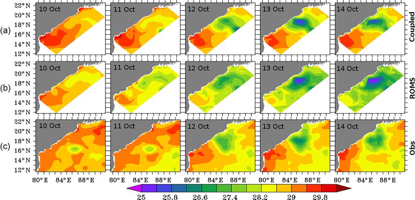
262                          K. R. Prakash et al.: Estimation of oceanic subsurface mixing under a severe cyclonic storm

moment (WSM) six-class moisture microphysics scheme by
Hong and Lim (2006). The sub-grid-scale convection and
cloud detrainment were taken care of with the Kain (2004)
cumulus scheme.
   The terrain-following ocean model ROMS with 40 sigma
levels in the vertical was used in this study. The ROMS model
domain was used with zonal and meridional grid resolutions
of 6 and 4 km, respectively. This high resolution in ROMS
enables us to resolve mesoscale eddies in the ocean. The ver-
tical stretching parameters, i.e., θs and θb were set to 7 and
2, respectively. The northern lateral boundary in ROMS was
represented by the Indian subcontinent. The ROMS model
observed open lateral boundaries in the west, east, and south
in the present configuration. The initial and lateral open
boundary conditions were derived from the Estimating the
Circulation and Climate of the Ocean, Phase II (ECCO2)
data (Menemenlis et al., 2005). The ocean bathymetry was
                                                                 Figure 2. The COAWST model domain (65–105◦ E, 1–34◦ N) over-
provided by the 2 min gridded global relief (ETOPO2) data
                                                                 laid with ETOPO2 bathymetry (m). Locations used for time series
(National Geophysical Data Center, 2006). There was no re-       analysis are marked with stars.
laxation provided for the model for any correction in the
temperature, salinity, and current fields. The generic length
scale (GLS) vertical mixing scheme parameterized as the K-       mosphere, ocean, and wave models at every 600 s. The SST
ε model was used (Warner et al., 2005). Tidal boundary con-      simulation at high spatial and temporal resolutions enables
ditions were derived from the TPXO.7.2 (ftp://ftp.oce.orst.      accurate heat fluxes at the air–sea interface and the exchange
edu/dist/tides/Global) data, which include the phase and am-     of heat between the oceanic mixed layer and atmospheric
plitude of the M2, S2, N2, K2, K1, O1, P1, MF, MM, M4,           boundary layer. The surface roughness parameter calculated
MS4, and MN4 tidal constituents along the east coast of In-      in the WRF model is based on Taylor and Yelland (2001),
dia. The tidal input was interpolated from the TPXO.7.2 grid     which involved parameters from the wave model.
to the ROMS computational grid. The Shchepetkin bound-
ary condition (Shchepetkin and McWilliams, 2005) for the         2.3   Methodology
barotropic current was used at open lateral boundaries of the
domain, which allowed the free propagation of astronomi-         The baroclinic current component was calculated by sub-
cal tide and wind-generated currents. The domains of the         tracting the barotropic component from the mean current
atmosphere and ocean models are shown in Fig. 2. ROMS            with a resolution of 2 m in the vertical. The power spectrum
and SWAN were configured over the common model domain            analysis was performed on the zonal and meridional baro-
shown with the shaded bathymetry data in Fig. 2. The two         clinic currents along the depth section of the selected loca-
locations used for the time series analysis are marked with      tions by using the periodogram method (Auger and Flandrin,
stars in Fig. 2. These two locations, one on-track and another   1995). The continuous wavelet transform using the Morlet
off-track, were selected in the vicinity of the region of max-   wavelet method (Lilly and Olhede, 2012) was carried out to
imum surface cooling and wind stress during the passage of       analyze the temporal variability in the baroclinic current at
Phailin. The wave model SWAN was forced with the WRF-            a particular level of 14 m. The near-inertial baroclinic veloc-
computed wind field. We used 24 frequency (0.04–1.0 Hz)          ities were filtered by the Butterworth second-order scheme
and 36 directional bands in the SWAN model. The bound-           for the cutoff frequency range of 0.028 to 0.038 cycle h−1 .
ary conditions for SWAN were derived from the WaveWatch          The filtered zonal (uf ) and meridional (vf ) inertial baroclinic
III model. In the COAWST system, the free-surface eleva-         currents were used to calculate the inertial baroclinic kinetic
tions (ELV) and current (CUR) simulated by the ocean model       energy (Ef ) in m2 s−2 and inertial shear (Sf ) following Zhang
ROMS are provided for the wave model SWAN. The Kirby             et al. (2014) and using Eq. (1).
and Chen (1998) formulation was used for the computation
of currents. The surface wind applied to the SWAN model                    ∂uf 2   ∂vf 2
                                                                 Sf2 = (      ) +(    )                                       (1)
(provided by WRF) was used in the Komen et al. (1984)                      ∂z      ∂z
closure model to transfer energy from the wind to the wave       As the stratification is a measure of oceanic stability, the
field. The baroclinic time step used in the ROMS model was       buoyancy frequency (N) was calculated using Eq. (2):
5 s. The SWAN and WRF models were used with time steps
of 120 and 60 s, respectively. The coupled modeling system                  g ∂ρ
allows the exchange of prognostic variables among the at-        N2 = −          ,                                            (2)
                                                                            ρ ∂z

Ocean Sci., 14, 259–272, 2018                                                                www.ocean-sci.net/14/259/2018/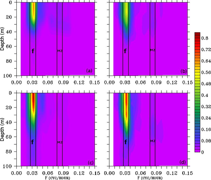
K. R. Prakash et al.: Estimation of oceanic subsurface mixing under a severe cyclonic storm 263
Figure 3. Tracks of Phailin simulated by the coupled model (black)
and IMD reported (red). The 3-hourly positions of the center of
Phailin are marked with solid circles, and the daily position at
00:00 h is labeled with the dates. Location of buoy BD09 is marked
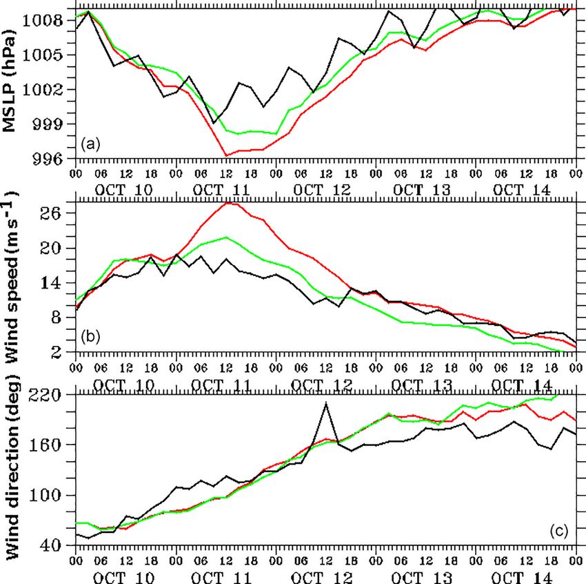
with a blue circle. Figure 4. Comparison of coupled model (green), stand-alone WRF
model (red), and observations from a buoy BD09 (black) for the (a)
mean sea level pressure (hPa), (b) wind speed (m s−1 ), and (c) wind
where ρ is the density of seawater and g is the acceleration direction (degree).
due to gravity.
The analysis of the generation of the inertial oscillations
and their dissipation was performed on the basis of turbu-
lent dissipation rate () and turbulent eddy diffusivity (kρ ). to the IMD track of Phailin. The stand-alone WRF model
These parameters were calculated by using the following for- (not shown here) was found to simulate Phailin’s track in
mula (Mackinnon and Gregg, 2005; van der Lee and Umlauf, an almost identical way to the WRF in the coupled config-
2011; Palmer et al., 2008; Osborn, 1980): uration. However, the intensity (surface wind speed) in the
WRF stand-alone model was higher compared to the cou-
N Slf pled model. Figure 4 shows the comparison of stand-alone
ε = ε0 , (3)
N0 S0 and coupled WRF model-simulated mean sea level pressure
ε
(MSLP), wind speed, and wind direction at a buoy (BD09)
kρ = 0.2 × , (4)
N2 location (marked with a blue circle in Fig. 3). It can be in-
ferred from the figure that stand-alone WRF simulated a
where Slf is the low shear background velocity and N0 = larger pressure drop and higher wind speed compared to
S0 = 3 cycle per hour and ε0 = 10−8 W kg−1 . buoy measurements. In addition to the cyclone-induced pres-
sure drop during 10–12 October, the semidiurnal variations
3 Results and discussion in MSLP were observed in the buoy measurements. These
semidiurnal variations in MSLP, primarily due to the radia-
3.1 Validation of coupled model simulations tional forcing (Pugh, 1987), were not captured by the model
over the cyclone-influenced region. The WRF in coupled
The WRF model-simulated track of Phailin was validated model configuration shows better performance in simulating
against the India Meteorological Department (IMD) reported the surface wind speed and pressure during Phailin. The ex-
best track of the cyclone. A comparison of the model- change of wave parameters with the WRF model in the cou-
simulated track with the IMD track is shown in Fig. 3. Solid pled configuration provides realistic sea surface roughness
circles marked on both the tracks represent the 3-hourly po- that resulted in the improvement of surface wind speed.
sitions of the cyclone’s center, as identified by the mini- The SST simulated by the ROMS model in coupled and
mum surface pressure. The daily positions of the center of stand-alone configurations was validated against the Ad-
Phailin are labeled with the date. The WRF model in the vanced Very High Resolution Radiometer (AVHRR) satel-
coupled configuration does a fairly good job of simulating lite data on each day for the period of Phailin’s passage over
the track, translational speed, and landfall location of Phailin. the BoB. The stand-alone WRF-simulated parameters were
The positional track error was about 40 km when compared used to provide surface boundary conditions in the stand-
www.ocean-sci.net/14/259/2018/ Ocean Sci., 14, 259–272, 2018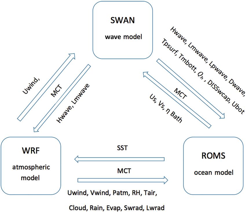
264                           K. R. Prakash et al.: Estimation of oceanic subsurface mixing under a severe cyclonic storm

Figure 5. The daily averaged sea surface temperature (SST) in ◦ C simulated by the coupled model (a) and stand-alone ROMS model (b) and
observed from AVHRR sensor on the satellite (c).

alone ROMS model. Figure 5 shows that the coupled model               track location leads to greater mixing, resulting in a deeper
captures the SST spatial pattern reasonably well with about           mixed layer on 12 October compared to the on-track location.
−0.5 ◦ C bias in northwestern BoB on 13–14 October. This              The surface wind speed at the on-track location shows typi-
order of bias in SST could result from the errors in initial          cal temporal variation in a passing cyclone. The wind speed
and boundary conditions provided for the model. The max-              peaks, drops, and attains a second peak as the cyclone ap-
imum cooling of the sea surface was observed on 13 Octo-              proaches, crosses over, and departs the location. The surface
ber in the northwestern BoB in both the coupled model and             currents forced by these large variations in wind speed and
observations. This post-cyclone cooling is primarily associ-          direction at the on-track location result in a comparatively
ated with the cyclone-induced upwelling resulting from the            weaker magnitude than the off-track location.
surface divergence driven by the Ekman transport. Thus, the              The thermocline, defined as the depth of maximum tem-
coupled model reproduces dynamical processes and vertical             perature gradient, is usually given with reference to the
velocities reasonably well. The stand-alone ROMS model                location-dependent isotherm depth (Kessler, 1990; Wang et
overestimates the cyclone-induced cooling with a −2.2 ◦ C             al., 2000). Over the BoB region, the depth of the 23 ◦ C
bias in SST on 13–14 October (Fig. 5). The stronger surface           isotherm (D23) was found to be an appropriate representative
winds in the stand-alone WRF cause the larger cold bias in            depth of the thermocline (Girishkumar et al., 2013). Based
the stand-alone ROMS model.                                           on the density criteria, we calculated the oceanic mixed
                                                                      layer depth (MLD) as the depth where density increased by
3.2   Cyclone-induced mixing                                          0.125 kg m−3 from its surface value. The inertial mixing in-
                                                                      troduced by the cyclone plays a central role in the deepening
The coupled atmosphere–ocean–wave simulation is an ideal              of D23 and MLD on 12 October 2013. The warmer near-
tool to understand the air–sea exchange of fluxes and their           surface waters mixed downward when the cyclone crossed
effects on the oceanic water column. Surface wind sets up             over this location. After the passage of cyclone, shoaling of
currents on the surface as well as initiating mixing in the in-       D23 and MLD has observed as a consequence of cyclone-
terior of the upper ocean. In order to examine the strength           induced upwelling that entrained colder waters from the ther-
of mixing due to Phailin, the model-simulated vertical tem-           mocline into the mixed layer. The temperature of the upper
perature profile together with the surface wind speed, zonal          surface water (25–30 m) decreased by 3.5 ◦ C from its maxi-
and meridional components of the current, and kinetic energy          mum value of 28 ◦ C after the landfall of the cyclone on 12–13
at the on-track and off-track locations are plotted in Fig. 6.        October at the off-track location (Fig. 6g). In response to the
Comparatively stronger zonal and meridional currents were             strong cyclonic winds, the D23 deepening by 40 m (from 50
observed at the off-track location than the on-track location         to 90 m) was observed during 04:00–12:00 GMT on 12 Oc-
on 12 October. The larger kinetic energy available at the off-

Ocean Sci., 14, 259–272, 2018                                                                      www.ocean-sci.net/14/259/2018/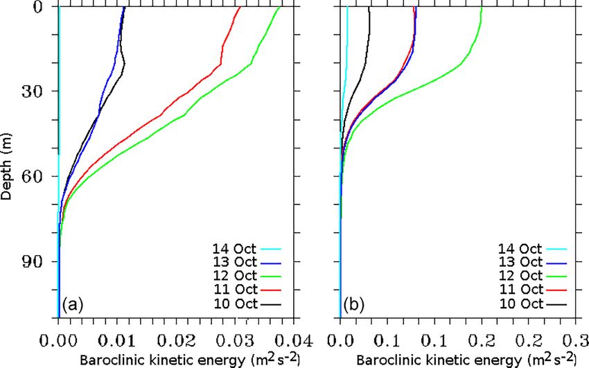
K. R. Prakash et al.: Estimation of oceanic subsurface mixing under a severe cyclonic storm                                            265

Figure 6. Coupled model-simulated and diagnosed variables at the on-track (left panel) and off-track (right panel) locations. (a, f) Surface
wind speed (m s−1 ); (b, g) temperature profile (◦ C) and mixed layer depth (black line); (c, h) u-component of current (m s−1 ); (d, i)
v-component of current (m s−1 ); (e, j) kinetic energy of the baroclinic (m2 s−2 ) and barotropic (× 10−2 m2 s−2 ) current.

tober. At the same time, the MLD, denoted by a thick black              (Fig. 6). The frequency of these reversals in zonal and merid-
line in Fig. 6g, deepens by about 15 m. On the other hand,              ional currents is recognized as a near-inertial frequency gen-
the on-track location showed cooling at the surface only for            erated from the storm at these locations. The direction and
a short time on 13 October, and the deepening of D23 and                magnitude of currents represent a variability that corresponds
MLD were 20 and 10 m, respectively. To examine the role                 to the presence of near-inertial oscillations at the selected lo-
of cyclone-induced mixing in modulating the thermohaline                cations. The kinetic energy (KE) of currents at various depths
structure of the upper ocean, we carried out further analysis           is a proxy of energy available in the water column that be-
on the coupled model simulations as discussed in the follow-            comes conducive to turbulent and inertial mixing. Time se-
ing sections.                                                           ries of KE associated with the barotropic and depth-averaged
                                                                        baroclinic components of the current at the two point loca-
3.2.1   Kinetic energy distribution                                     tions are illustrated in Fig. 6e (on-track) and 6j (off-track).
                                                                        The KE associated with the baroclinic component was found
During the initial phase of Phailin, the zonal and meridional           to be much higher than the barotropic component of current
currents were primarily westward and southward, respec-                 at both on-track and off-track locations. The depth-averaged
tively (Fig. 6c, d, h, and i). However, on and after 12 October         baroclinic and barotropic current components’ KE also de-
when the cyclone attained peak intensity and crossed over               pict the impinging oscillatory behavior. The peak magnitude
the location, alternative temporal sequences running west-              of KE in baroclinic and barotropic currents at the off-track
ward/eastward in the zonal current and southward/northward              location was found to be 1.2 m2 s−2 and 0.3 × 10⁻² m2 s−2 ,
in the meridional current were noticed in current profiles              respectively, on 12 October at 08:00 GMT, whereas the mag-

www.ocean-sci.net/14/259/2018/                                                                           Ocean Sci., 14, 259–272, 2018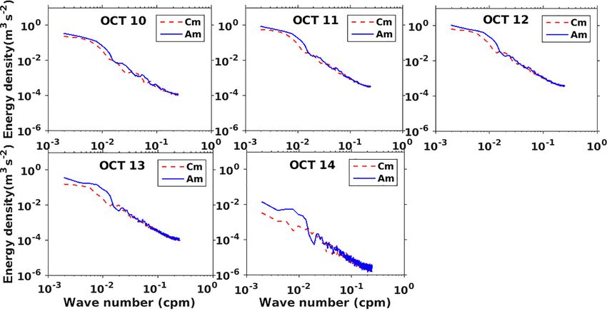
266                           K. R. Prakash et al.: Estimation of oceanic subsurface mixing under a severe cyclonic storm

nitude of KE in baroclinic and barotropic currents at the on-
track location was smaller than the off-track location during
the peak intensity of the cyclone. The peak magnitude of ki-
netic energy in the baroclinic current at the off-track location
was more than double that of on-track location. The com-
paratively smaller magnitude of KE at the on-track location
could be associated with the rapid variations in wind speed
and direction leading to the complex interaction between
subsurface currents in the central region of the cyclone. It is
worth noting that the time of peak KE in baroclinic currents
coincides with the deepening of MLD and D23. Therefore,
the KE generated in NIO is responsible for subsurface mix-
ing that acts to deepen the mixed layer. The analysis suggests
that energy available for the mixing process in the water col-
umn was mostly confined to the baroclinic currents at various
depths.

3.2.2   Primary frequency and depth of mixing
                                                                    Figure 7. The power spectrum analysis (m2 s−1 ) performed on the
The power spectrum analysis was performed on the time se-           simulation period at the on-track (upper panel) and off-track (lower
                                                                    panel) locations for (a, c) the baroclinic zonal current and (b, d) the
ries profiles at the two selected locations to get a distribution
                                                                    baroclinic meridional current.
of all frequencies operating in the mixing process during the
passage of Phailin. The power spectrum analysis was per-
formed on the zonal and meridional components of the baro-          the frequency range of 0.028 to 0.038 cycles h−1 at the se-
clinic current profile and shown in Fig. 7. It is clear from        lected locations. The filtered baroclinic current was further
the figure that the tidal (M2, the semidiurnal component of         utilized to calculate the filtered inertial baroclinic KE (Ef in
tide) and near-inertial oscillations (f) are the two dominant       m2 s−2 ). The daily profiles of baroclinic KE were analyzed
frequencies on the surface during cyclone Phailin. Under the        at the two selected locations and shown in Fig. 8. The peak
influence of cyclonic winds, the NIO signal was stronger            baroclinic KE differs from 0.14 m2 s−2 at the on-track to
(0.84 m2 s−2 ) at the off-track than the on-track location. The     0.23 m2 s−2 at the off-track location on 12 October. As shown
depth penetration of NIO was up to 50 and 35 m at the off-          in Figs. 6 and 7, the filtered baroclinic KE profiles (Fig. 8)
track and on-track location, respectively. The tidal frequency      confirm the dominant presence of NIO at the off-track loca-
(M2) and inertial frequency (f) bands shown in Fig. 7 im-           tion compared to the on-track location. The decay of NIO
plies that the inertial oscillations were dominant over the tidal   with the increasing depth was noticed at both the locations.
constituent in zonal and meridional baroclinic currents. At         However, the NIO baroclinic KE penetrated up to 80 m in
the off-track location, the largest power of the NIO was no-        the case of an off-track location as compared to only 50 m at
ticed at 14 m depth, but the tidal oscillations were almost ab-     the on-track location. The analysis, therefore, suggests that
sent in the vertical section of baroclinic current (Fig. 7). This   the NIOs generated during Phailin were more energetic at
finding motivated us to analyze the significance and distribu-      the selected off-track location, which was also the location
tion of this subsurface variability that resulted in an anoma-      of maximum surface cooling as noted in Fig. 5. Therefore,
lous deepening of MLD. The highest power of this signal             the further analysis in the subsequent sections is limited to
at the off-track location was associated within 0–15 m, with        the off-track location only. To analyze the time distribution
a magnitude of 0.84 m2 s−1 in the zonal baroclinic current,         of the strong NIO, wavelet transform analysis was applied to
and within 0–38 m, with a magnitude of 0.76 m2 s−1 in the           the zonal and meridional baroclinic currents at 14 m depth.
meridional baroclinic current. These signals, however, weak-        The scalogram, shown in Fig. 9, depicts the generation of
ened with increasing depth and almost disappeared around            NIO signal at the off-track location on 12 October that sub-
120 m depth. Compared to any other process, these NIOs              sequently strengthened and attained its peak value in the mid-
were the strongest signals at the 14 m depth in the presence        dle of the day on 13 October. The energy percentage of the
of local wind stress that dominated the mixing. Other pro-          meridional component was always lower than the zonal com-
cesses include the background flows, the presence of eddies,        ponent. The peak values of energy percentage were found in
variations in sea surface height, and nonlinear wave–wave           the time periods between 1 and 1.3 days.
and wave–current interactions (Guan et al., 2014; Park and
Watts, 2005).
   The second-order Butterworth filter was applied to the
baroclinic current components to get the strength of NIO in

Ocean Sci., 14, 259–272, 2018                                                                      www.ocean-sci.net/14/259/2018/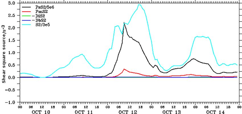
K. R. Prakash et al.: Estimation of oceanic subsurface mixing under a severe cyclonic storm                                         267

Figure 8. Daily averaged baroclinic kinetic energy (m2 s−2 ) profile
at the on-track (a) and off-track (b) locations as marked with stars
in Fig. 2.

3.2.3   Role of the downward propagation of energy                     Figure 9. The scalogram by continuous wavelet transform (CWT)
                                                                       method in percentage at 14 m depth . Wavelet scalogram shown for
To investigate the energy propagation from the surface to              the zonal baroclinic current (a) and for the meridional baroclinic
the interior layers of the upper ocean, we derived the ro-             current (b).
tary spectra (Gonella, 1972; Hayashi, 1979) of near-inertial
wave numbers shown in Fig. 10. The daily averaged verti-
cal wave-number rotary spectra provide a clear picture of              ing the magnitude of bulk shear during the stormy event. The
wind energy distribution in the subsurface water. The anticy-          rest of the terms were relatively weaker and, therefore, con-
clonic spectrum (Am ) dominates the cyclonic spectra (Cm )             tributed only marginally to the variability in the bulk shear.
for the entire duration of the cyclone. This feature indicates            To examine the generation and dissipation of these in-
that the energy generated by these inertial oscillations prop-         ertial oscillations, the shear generated by the near-inertial
agates downward. The magnitude of these oscillations in-               baroclinic current (Sf2 ) and turbulent kinetic energy dissipa-
creased from the initial stage up to 12 October and remained           tion rate (ε) was calculated and analyzed. The shear pro-
at a high energy density for the rest of the cyclone period.           duced by inertial oscillations increased at 20–80 m depth,
This downward-directed energy initiated a process of mixing            and a higher magnitude was associated with the peak wind
between the mixed layer and the thermocline. This energy               speed of the cyclone (Fig. 12a). This shear overcame the
helps to deepen the mixed layer against oceanic stratification         stratification (Fig. 12b), represented by buoyancy frequency
by introducing a strong shear. The buoyancy of the strati-             N 2 , and played important role in the mixing and deepen-
fied ocean was overcome to some extent by the shear gener-             ing of the thermocline and mixed layer on 12 October. The
ated, which assisted in the mixing process during the very             value of the kinetic energy dissipation rate (ε) increased from
severe cyclone. Alford and Gregg (2001) highlighted that               4×10⁻¹⁴ to 2.5×10⁻¹³ W kg−1 on approaching the thermo-
in most of the cases, the energy of inertial oscillations po-          cline (Fig. 12c). The increase in ε indicates the weakening
tentially penetrates the mixed layer but suddenly drops as it          of the shear generated by the inertial waves leading to the
touches the thermocline. The energy dissipation mechanism              fast disappearance of these baroclinic instabilities from the
has been studied in a few other studies (Chant, 2001; Jacob            region. The nonlinear interaction between the NIO and in-
and Shay, 2003). The two-layer model described by Burchard             ternal tides together with the prevailing background currents
and Rippeth (2009) illustrated the process of the generation           causes the rapid dissipation of kinetic energy in the thermo-
of sufficient shear to start mixing near the thermocline. Their        cline. Guan et al. (2014) also reported an accelerated damp-
simple model ignored the effect of the lateral density gra-            ening of NIO associated with the wave–wave interactions be-
dient, mixing, and advection. Burchard et al. (2009) men-              tween NIO and internal tides. The background currents were
tioned four important parameters for shear generation, i.e.,           found to modify the propagation of NIO (Park and Watts,
surface wind stress (PS S 2 ), bed stress (−Db S 2 ), interfacial      2005). The magnitude of the turbulent eddy diffusivity (Kρ ),
stress (−DI S 2 ), and barotropic flow (Pm S 2 ). Utilizing sim-       shown in Fig. 12d, implies that the greater mixing takes place
ulations from our coupled atmosphere–ocean–wave model,                 within the mixed layer where Kρ was high (6.3 × 10⁻¹¹ to
we calculated individual terms as suggested by Burchard et             1.2 × 10⁻¹¹ m2 s−1 ). The daily averaged values of ε and Kρ
al. (2009), and we present them in Fig. 11. Surface wind               were 1.2 × 10⁻¹³ W kg−1 and 1.5 × 10⁻¹⁰ m2 s−1 , respec-
stress was found to be the most dominating term in modulat-            tively, on 12 October, which were higher compared to the

www.ocean-sci.net/14/259/2018/                                                                        Ocean Sci., 14, 259–272, 2018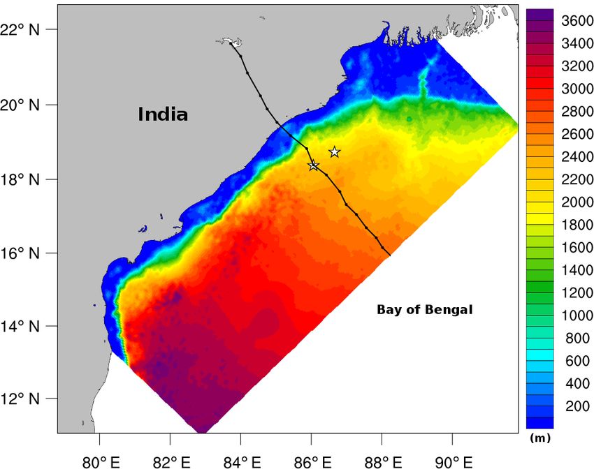
268                            K. R. Prakash et al.: Estimation of oceanic subsurface mixing under a severe cyclonic storm

Figure 10. The daily averaged vertical wave-number rotary spectra of near-inertial oscillations. The anticyclonic and cyclonic spectra are
represented by blue and dotted red lines, respectively.

Figure 11. The model-simulated bulk properties at the selected point location. The vertical shear square axis is multiplied by a factor of
10−6 . The magnitude of bulk shear squared S 2 (cyan color), surface wind stress Ps S 2 (black color), barotropic effect Pm S 2 (red color),
bottom stress – Db S 2 (blue color), and interfacial friction – Di S 2 (green color) are shown for the duration of the cyclone.

initial 2 days of the cyclonic event. Results from the present          Phailin cyclone. A detailed analysis of model-simulated data
study, as well as conclusions from past studies, indicate that          revealed interesting features of generation, propagation, and
wave–current interaction, mesoscale processes, and wave–                dissipation of kinetic energy in the upper-oceanic water col-
wave interaction can affect the process of downward mixing              umn. The deepening of the MLD and thermocline by 15 and
and cause the dissipation of inertial oscillations.                     40 m, respectively, was explained through the strong shear
                                                                        generated by the inertial oscillations that helped to overcome
                                                                        the stratification and initiate mixing at the base of the mixed
4   Conclusions                                                         layer. However, there was a rapid dissipation of the shear
                                                                        with increasing depth below the thermocline. The peak mag-
Processes controlling the subsurface mixing were evalu-                 nitude of kinetic energy in baroclinic and barotropic currents
ated under the high wind speed regime of the severe cy-                 was found to be 1.2 and 0.3 × 10⁻² m2 s−2 , respectively. The
clonic storm Phailin over the BoB. A coupled atmosphere–                power spectrum analysis suggested a dominant frequency op-
ocean–wave (WRF+ROMS+SWAN) model as part of the                         erative in subsurface mixing that was associated with near-
COAWST modeling system was used to simulate atmo-                       inertial oscillations. The peak strength of 0.84 m2 s−1 in the
spheric and oceanic conditions during the passage of the

Ocean Sci., 14, 259–272, 2018                                                                         www.ocean-sci.net/14/259/2018/
K. R. Prakash et al.: Estimation of oceanic subsurface mixing under a severe cyclonic storm 269
Figure 12. Profiles of (a) velocity shear log10 (S 2 ), (b) buoyancy frequency log10 (N 2 ), (c) turbulent kinetic energy dissipation rate log10
(ε), and (d) turbulent eddy diffusivity log10 (Kρ ); (e) and (f) are daily averaged turbulent kinetic energy dissipation rate and turbulent eddy
diffusivity, respectively.
zonal baroclinic current was found at 14 m depth at a lo- ing of the oceanic response under strong wind conditions.
cation in the northwestern BoB. The baroclinic kinetic en- The proper representation of kinetic energy propagation and
ergy remained higher (> 0.03 m2 s−2 ) during 11–12 Octo- oceanic mixing have applications in improving the intensity
ber and decreased rapidly after that. The wave-number ro- prediction of a cyclone, storm surge forecasting, and biolog-
tary spectra identified the downward propagation, from the ical productivity.
surface up to the thermocline, of energy generated by iner-
tial oscillations. A quantitative analysis of shear generated
by the near-inertial baroclinic current showed higher shear Data availability. The atmospheric and ocean model forcing data
generation at 20–80 m depth during peak surface winds. can be obtained from FNL (https://rda.ucar.edu/datasets/ds083.2/;
Analysis highlights that greater mixing within the mixed NCEPFNL, 2000) and ECCO2 (https://ecco.jpl.nasa.gov/products/
layer takes place where the eddy kinetic diffusivity is high all/, last access: October 2016), respectively. The observation
data utilized for model validation are obtained from Indian Na-
(> 6 × 10⁻¹¹ m2 s−1 ). The turbulent kinetic energy dissipa-
tional Centre for Ocean Information Services (http://www.incois.
tion rate increased from 4 × 10⁻¹⁴ to 2.5 × 10⁻¹³ W kg−1 on
gov.in/portal/index.jsp, last access: February 2017). The model
approaching the thermocline, which dampened the mixing simulations used for the research article can be obtained from
process further down into the thermocline layer. The wave– the first author, Kumar Ravi Prakash, by sending an email to
current interaction, mesoscale processes, and wave–wave in- kravi1220@gmail.com.
teraction increased the dissipation rate of shear and, thereby,
limited the downward mixing up to the thermocline. The cou-
pled model was found to be a useful tool to investigate air– Author contributions. KRP and TN performed model simulations
sea interaction, kinetic energy propagation, and mixing in the and analyzed data. VP prepared the manuscript with contributions
upper ocean. The results from this study highlight the impor- from all co-authors.
tance of atmosphere–ocean coupling for a better understand-
www.ocean-sci.net/14/259/2018/ Ocean Sci., 14, 259–272, 2018270 K. R. Prakash et al.: Estimation of oceanic subsurface mixing under a severe cyclonic storm
Competing interests. The authors declare that they have no conflict Dudhia, J.: Numerical study of convection observed during the
of interest. winter monsoon experiment using a mesoscale two dimensional
model, J. Atmos. Sci., 46, 3077–3107, 1989.
Gill, A. E.: On the behavior of internal waves in the wake of storms,
Acknowledgements. ECCO2 is a contribution to the NASA Model- J. Phys. Oceanogr., 14, 1129–1151, 1984.
ing, Analysis, and Prediction (MAP) program. The study benefitted Girishkumar, M. S., Ravichandran, M., and Han, W.: Ob-
from the funding support from the Ministry of Earth Sciences, served intraseasonal thermocline variability in the Bay
Government of India, and the Space Applications Centre, Indian of Bengal, J. Geophys. Res.-Oceans, 118, 3336–3349,
Space Research Organisation. The high-performance computing https://doi.org/10.1002/jgrc.20245, 2013.
(HPC) facility provided by IIT Delhi and the Department of Gonella, J.: A study of inertial oscillations in the upper layers of the
Science and Technology (DST-FIST 2014 at CAS), Government oceans, Deep-Sea Res., 18, 775–788, 1971.
of India, are thankfully acknowledged. Authors are thankful Gonella, J.: A rotary-component method for analysing meteorolog-
to Lingling Xie for his productive suggestions. Graphics were ical and oceanographic vector time series, Deep-Sea Res., 19,
generated in this paper using Ferret and NCL. The constructive 833–846, 1972.
comments from three anonymous reviewers helped to improve the Gröger, M., Dieterich, C., Meier, H. E. M., and Schimanke, S.:
paper. Tanuja Nigam and Kumar Ravi Prakash acknowledge MoES Thermal air-sea coupling in hindcast simulations for the North
and UGC-CSIR, respectively, for their PhD fellowship support. Sea and Baltic Sea on the NW European shelf, Tellus A, 67,
26911, https://doi.org/10.3402/tellusa.v67.26911, 2015.
Edited by: Markus Meier Guan, S., Zhao, W., Huthnance, J. Tian, J., and Wang, J.: Observed
Reviewed by: three anonymous referees upper ocean response to typhoon Megi (2010) in the Northern
South China Sea, J. Geophys. Res.-Oceans, 119, 3134–3157,
https://doi.org/10.1002/2013JC009661, 2014.
Haidvogel, D. B., Arango, H. G., Hedstrom, K., Beckmann, A.,
Malanotte-Rizzoli, P., and Shchepetkin, A. F.: Model evaluation
References experiments in the North Atlantic Basin: Simulations in nonlin-
ear terrain-following coordinates, Dyn. Atmos. Oceans, 32, 239–
Alam, M. M., Hossain, M. A., and Shafee, S.: Frequency 281, 2000.
of Bay of Bengal cyclonic storms and depressions cross- Haidvogel, D. B., Arango, H. G., Budgell, W. P., Cornuelle, B. D.,
ing different coastal zones, Int. J. Climatol., 23, 1119–1125, Curchitser, E., Di Lorenzo, E., Fennel, K., Geyer, W. R., Her-
https://doi.org/10.1002/joc.927, 2003. mann, A. J., Lanerolle, L., Levin, J., McWilliams, J. C., Miller, A.
Alford, M. H. and Gregg, M. C.: Near-inertial mixing: modulation J., Moore, A. M., Powell, T. M., Shchepetkin, A. F., Sherwood,
of shear, strain and microstructure at low latitude, J. Geophys. C. R., Signell, R. P., Warner, J. C., and Wilkin, J.: Regional ocean
Res., 106, 16947–16968, 2001. forecasting in terrain-following coordinates: model formulation
Auger, F. and Flandrin, P.: Improving the Readability of Time- and skill assessment, J. Comput. Phys., 227, 3595–3624, 2008.
Frequency and Time-Scale Representations by the Reassignment Hayashi, Y.: Space-time spectral analysis of rotary vector series, J.
Method, IEEE Transactions on Signal Processing, 43, 1068– Atmos. Sci., 36, 757–766, 1979.
1089, 1995. Ho-Hagemann, H. T. M., Gröger, M., Rockel, B., Zahn, M.,
Booij, N., Ris, R. C., and Holthuijsen, L. H.: A third- Geyer, B., and Meier, H. E. M: Effects of air-sea coupling
generation wave model for coastal regions, Part I, Model de- over the North Sea and the Baltic Sea on simulated sum-
scription and validation, J. Geophys. Res., 104, 7649–7666, mer precipitation over Central Europe, Clim. Dyn., 49, 3851,
https://doi.org/10.1029/98JC02622, 1999. https://doi.org/10.1007/s00382-017-3546-8, 2017.
Burchard, H. and Rippeth, T. P.: Generation of bulk shear spikes Hong, S. Y. and Lim, J. O. J.: The WRF single-moment 6-class
in shallow stratified tidal seas, J. Phys. Oceanogr., 39, 969–985, microphysics scheme (WSM6), J. Korean Meteor. Soc., 42, 129–
2009. 151, 2006.
Chang, S. W. and Anthes, F. A.: The mutual response of the tropical IMD Report: Very Severe Cyclonic Storm, PHAILIN over the Bay
cyclone and the ocean, J. Phys. Oceanogr., 9, 128–135, 1979. of Bengal (08–14 October 2013) A Report, India Meteorological
Chant, R. J.: Evolution of near-inertial waves during an upwelling Department, Technical Report, October 2013.
event on the New Jersey Inner Shelf, J. Phys. Oceanogr., 31, 746– Jacob, S. D. and Shay, L. K.: The role of oceanic mesoscale features
764, 2001. on the tropical cyclone-induced mixed layer response: A case
Chassignet, E. P., Arango, H. G., Dietrich, D., Ezer, T., Ghil, M., study, J. Phys. Oceanog., 33, 649–676, 2003.
Haidvogel, D. B., Ma, C. C., Mehra, A., Paiva, A. M., and Sirkes, Jacob, R., Larson, J., and Ong, E.: M x N Communication and
Z.: DAMEE-NAB: the base experiments. Dyn. Atmos. Oceans, Parallel Interpolation in CCSM Using the Model Coupling
32, 155–183, 2000. Toolkit, Preprint ANL/MCSP1225-0205, Mathematics and Com-
Chen, S., Chen, D., and Xing, J.: A study on some basic features of puter Science Division, Argonne National Laboratory, 25 pp.,
inertial oscillations and near-inertial internal waves, Ocean Sci., 2005.
13, 829–836, https://doi.org/10.5194/os-13-829-2017, 2017. Jeworrek, J., Wu, L., Dieterich, C., and Rutgersson, A.: Character-
Cione, J. J. and Uhlhorn, E. W.: Sea surface tempera- istics of convective snow bands along the Swedish east coast,
ture variability in hurricanes: Implications with respect to Earth Syst. Dynam., 8, 163–175, https://doi.org/10.5194/esd-8-
intensity change, Mon. Weather Rev., 131, 1783–1796, 163-2017, 2017.
https://doi.org/10.1175//2562.1, 2003.
Ocean Sci., 14, 259–272, 2018 www.ocean-sci.net/14/259/2018/K. R. Prakash et al.: Estimation of oceanic subsurface mixing under a severe cyclonic storm 271 Johnston, T. M. S., Chaudhuri, D., Mathur, M., Rudnick, D. available at: https://doi.org/10.7289/V5J1012Q (last access: July L., Sengupta, D., Simmons, H. L., Tandon, A., and Venkate- 2015), 2006. san, R.: Decay mechanisms of near-inertial mixed layer os- Neetu, S., Lengaigne, M., Vincent, E. M., Vialard, J., Madec, G., cillations in the Bay of Bengal, Oceanography, 29, 180–191, Samson, G., Ramesh Kumar, M. R., and Durand, F.: Influence https://doi.org/10.5670/oceanog.2016.50, 2016. of upper-ocean stratification on tropical cyclone-induced surface Kain, J. S.: The Kain-Fritsch convective parameterization: An up- cooling in the Bay of Bengal, J. Geophys. Res., 117, C12020, date, J. Appl. Meteor., 43, 170–181, 2004. https://doi.org/10.1029/2012JC008433, 2012. Kessler, W. S.: Observations of long Rossby waves in the northern Noh, Y., Cheon, W. G., Hong, S. Y., and Raasch, S.: Improvement tropical Pacific, J. Geophys. Res., 95, 5183–5217, 1990. of the K-profile model for the planetary boundary layer based on Kirby, J. T. and Chen, T. M.: Surface waves on vertically sheared large eddy simulation data, Bound. Layer Meteor., 107, 401–427, flows Approximate dispersion relations, J. Geophys. Res., 94, 2003. 1013–1027, https://doi.org/10.1029/JC094iC01p01013, 1989. Osborn, T. R.: Estimates of the Local-Rate of Vertical Diffusion Komen, G. J., Hasselmann, S., and Hasselmann, K.: On the exis- from Dissipation Measurements, J. Phys. Oceanogr., 10, 83–89, tence of a fully developed wind-sea spectrum, J. Phys. Oceanogr., 1980. 14, 1271–1285, 1984. Palmer, M. R., Rippeth, T. P., and Simpson, J. H.: An investigation Larson, J., Jacob, R., and Ong, E.: The Model Coupling Toolkit: A of internal mixing in a seasonally stratified shelf sea, J. Geophys. New Fortran90 Toolkit for Building Multiphysics Parallel Cou- Res., 113, C12005, https://doi.org/10.1029/2007JC004531, pled Models, Preprint ANL/MCS- P1208-1204, Mathematics 2008. and Computer Science Division, Argonne National Laboratory, Pant, V., Girishkumar, M. S., Udaya Bhaskar, T. V. S., Ravichan- 25 pp., 2004. dran, M., Papa, F., and Thangaprakash, V. P.: Observed interan- Leipper, D. F.: Observed Ocean Conditions and Hurricane Hilda, nual variability of near-surface salinity in the Bay of Bengal, J. 1964, J. Atmos. Sci., 24, 182–186, https://doi.org/10.1175/1520- Geophys. Res., 120, 3315–3329, 2015. 0469(1967)0242.0.CO;2, 1967. Park, J. H. and Watts, D. R.: Near-inertial oscillations in- Li, Z., Yu, W., Li, T., Murty, V. S. N., and Tangang, F.: Bimodal teracting with mesoscale circulation in the southwest- character of cyclone climatology in the Bay of Bengal modu- ern Japan/East Sea, Geophys. Res. Lett., 32, L10611, lated by monsoon seasonal cycle, J. Climate, 26, 1033–1046, https://doi.org/10.1029/2005GL022936, 2005. https://doi.org/10.1175/JCLI-D-11-00627.1, 2013. Prakash, K. R. and Pant, V: Upper oceanic response to trop- Lilly, J. M. and Olhede, S. C.: Generalized Morse Wavelets as a ical cyclone Phailin in the Bay of Bengal using a cou- Superfamily of Analytic Wavelets, IEEE Transactions on Signal pled atmosphere-ocean model, Ocean Dynam., 67, 51–64, Processing, 60, 6036–6041, 2012. https://doi.org/10.1007/s10236-016-1020-5, 2017. Longshore, D.: Encyclopedia of Hurricanes, Typhoons, and Cy- Price, J. F.: Upper ocean response to a hurricane, J. Phys. Oceanog., clones, 468 pp., Checkmark, New York, 2008. 11, 153–175, 1981. Lukas, R. and Lindstrom, E.: The mixed layer of the western equa- Price, J. F., Mooers, C. N., and Van Leer, J. C.: Observation and torial Pacific Ocean, J. Geophys. Res., 96, 3343–3357, 1991. simulation of storm-induced mixed-layer deepening, J. Phys. MacKinnon, J. A. and Gregg, M. C.: Spring Mixing: Turbulence Oceanogr., 8, 582–599, and Internal Waves during Restratification on the New England doi10.1175/1520-0485(1978)0082.0.CO;2, Shelf, J. Phys. Oceanogr., 12, 2425–2443 2005. 1978. Mandal, M., Singh, K. S., Balaji, M., and Mohapatra, M.: Per- Pugh, D. T.: Tides, Surges and Mean Sea-Level, John Wiley & Sons, formance of WRF-ARW model in real-time prediction of Chichester, 472 pp., 1987. Bay of Bengal cyclone ‘Phailin’, Pure Appl. Geophys., 173, Rao, R. R. and Sivakumar, R.: Seasonal variability of sea https://doi.org/10.1007/s00024-015-1206-7, 2015. surface salinity and salt budget of the mixed layer of Menenenlis, D., Hill, C., Adcroft, A., Campin, J.-M., Cheng, B., the north Indian Ocean, J. Geophys. Res., 108, 3009, Clottl, B., Fukumori, I., Pheimbach, C., Henze, A., Kohl, T., Lee, https://doi.org/10.1029/2001JC000907, 2003. D., Stammer, J., Taft, and Zhang, J.: NASA supercomputer im- Sanford, T. B., Black, P. G., Haustein, J., Feeney, J. W., Forristall, proves prospects for ocean climate research, Eos Trans. AGU, G. Z., and Price, J. F.: Ocean response to a hurricane. Part I: 86, 89–96, https://doi.org/10.1029/2005EO090002, 2005. Observations, J. Phys. Oceanogr., 17, 2065–2083, 1987. Monin, A. S. and Obukhov, A. M. F.: Basic laws of turbulent mixing Sanil Kumar, V. and Anjali Nair, M.: Inter-annual variations in the surface layer of the atmosphere, Contrib. Geophys. Inst. in wave spectral characteristics at a location off the cen- Acad. Sci. USSR, 151, e187, 1954. tral west coast of India, Ann. Geophys., 33, 159–167, National Centers for Environmental Prediction/National Weather https://doi.org/10.5194/angeo-33-159-2015, 2015. Service/NOAA/U.S. (NCEPFNL): Department of Commerce, Schahinger, R. B.: Near inertial motion on the south Australian NCEP FNL Operational Model Global Tropospheric Analy- shelf, J. Phys. Oceanogr., 18, 492–504, 1988. ses, continuing from July 1999, Research Data Archive at Shay, L. K. and Elsberry, R. L.: Vertical structure of the ocean cur- the National Center for Atmospheric Research, Computational rent response to a hurricane, J. Phys. Oceanog., 19, 649–669, and Information Systems Laboratory, data set, available at: 1989. https://doi.org/10.5065/D6M043C6 (last access: 4 July 2015), Shay, L. K., Black, P., Mariano, A., Hawkins, J., and Elsberry, R.: 2000. Upper ocean response to hurricane Gilbert, J. Geophys. Res., 97, National Geophysical Data Center: 2-minute Gridded Global Relief 227–248, 1992. Data (ETOPO2) v2. National Geophysical Data Center, NOAA, www.ocean-sci.net/14/259/2018/ Ocean Sci., 14, 259–272, 2018
You can also read