Transport, properties, and life cycles of mesoscale eddies in the eastern tropical South Pacific - Ocean Science
←
→
Page content transcription
If your browser does not render page correctly, please read the page content below
Ocean Sci., 14, 731–750, 2018
https://doi.org/10.5194/os-14-731-2018
© Author(s) 2018. This work is distributed under
the Creative Commons Attribution 4.0 License.

Transport, properties, and life cycles of mesoscale eddies in the
eastern tropical South Pacific
Rena Czeschel1 , Florian Schütte1 , Robert A. Weller2 , and Lothar Stramma1
1 GEOMAR     Helmholtz Centre for Ocean Research Kiel, Düsternbrooker Weg 20, 24105 Kiel, Germany
2 Woods   Hole Oceanographic Institution (WHOI), 266 Woods Hole Rd, Woods Hole, MA 02543, USA

Correspondence: Rena Czeschel (rczeschel@geomar.de)

Received: 15 January 2018 – Discussion started: 31 January 2018
Revised: 14 May 2018 – Accepted: 9 July 2018 – Published: 31 July 2018

Abstract. The influence of mesoscale eddies on the flow            floats were trapped in the ACE2 during its westward prop-
field and the water masses, especially the oxygen distri-          agation between the formation region and the open ocean,
bution of the eastern tropical South Pacific, is investigated      which allows for conclusions on lateral mixing of water mass
from a mooring, float, and satellite data set. Two anticy-         properties with time between the core of the eddy and the
clonic (ACE1/2), one mode-water (MWE), and one cyclonic            surrounding water. The strongest lateral mixing was found
eddy (CE) are identified and followed in detail with satel-        between the seasonal thermocline and the eddy core during
lite data on their westward transition with velocities of 3.2 to   the first half of the eddy lifetime.
6.0 cm s−1 from their generation region, the shelf of the Peru-
vian and Chilean upwelling regime, across the Stratus Ocean
Reference Station (ORS; ∼ 20◦ S, 85◦ W) to their decaying
region far west in the oligotrophic open ocean. The ORS            1   Introduction
is located in the transition zone between the oxygen mini-
mum zone and the well oxygenated South Pacific subtropi-           The eastern tropical South Pacific (ETSP) containing the
cal gyre. Velocity, hydrographic, and oxygen measurements          Peruvian upwelling regime, which is one of the four ma-
at the mooring show the impact of eddies on the weak flow          jor eastern boundary upwelling systems, shows pronounced
region of the eastern tropical South Pacific. Strong anomalies     mesoscale and sub-mesoscale variability (e.g. Capet et al.,
are related to the passage of eddies and are not associated        2008; McWilliams et al., 2009; Chaigneau et al., 2011).
with a seasonal signal in the open ocean. The mass trans-          Mesoscale variability in the ocean occurs as linear Rossby
port of the four observed eddies across 85◦ W is between           waves and as nonlinear vortices or eddies. During the last
1.1 and 1.8 Sv. The eddy type-dependent available heat, salt,      two decades eddies have been recognized to play an impor-
and oxygen anomalies are 8.1 × 10¹⁸ J (ACE2), 1.0 × 10¹⁸ J         tant role in the vertical and horizontal transport of momen-
(MWE), and −8.9 × 10¹⁸ J (CE) for heat; 25.2 × 10¹⁰ kg             tum, heat, mass, and chemical constituents of seawater (e.g.
(ACE2), −3.1 × 10¹⁰ kg (MWE), and −41.5 × 10¹⁰ kg (CE)             Chelton et al., 2007; Klein and Lapeyre, 2009) and there-
for salt; and −3.6 × 10¹⁶ µmol (ACE2), −3.5 × 10¹⁶ µmol            fore contribute to the large-scale water mass distribution. Es-
(MWE), and −6.5 × 10¹⁶ µmol (CE) for oxygen showing a              pecially in upwelling areas, eddies have been identified as
strong imbalance between anticyclones and cyclones for salt        major agents for the exchange between coastal waters and
transports probably due to seasonal variability in water mass      the open ocean (e.g. Chaigneau et al., 2008; Pegliasco et al.,
properties in the formation region of the eddies. Heat, salt,      2015; Schütte et al., 2016a). At least three types of eddies
and oxygen fluxes out of the coastal region across the ORS         have been identified: cyclonic, anticyclonic, and anticyclonic
region in the oligotrophic open South Pacific are estimated        mode-water eddies (e.g. McWilliams, 1985; D’Asaro, 1988;
based on these eddy anomalies and on eddy statistics (gained       McGillicuddy Jr. et al., 2007), as well as a transition from
out of 23 years of satellite data). Furthermore, four profiling    cyclonic eddies to “cyclonic thinnies” to exist throughout the
                                                                   world ocean (McGillicuddy Jr., 2015). Usually, isopycnals

Published by Copernicus Publications on behalf of the European Geosciences Union.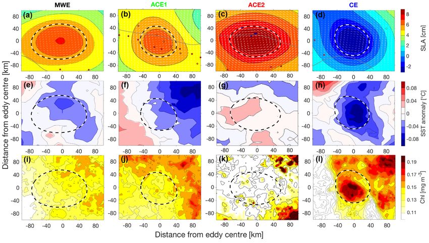
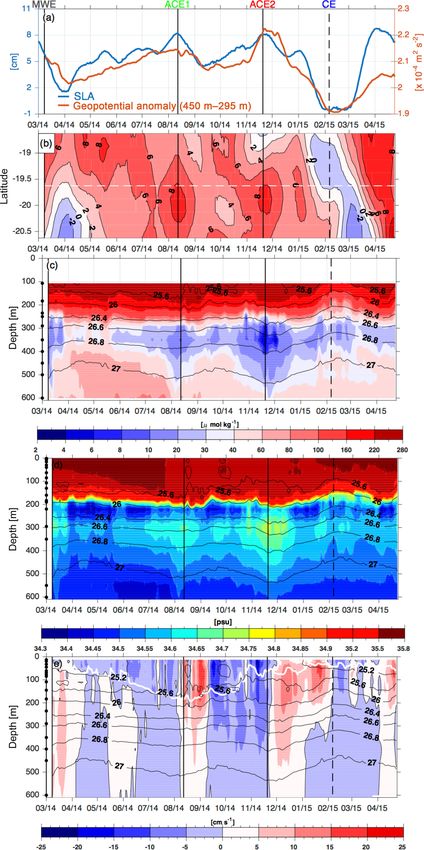
732                                                R. Czeschel et al.: Transport, properties, and life cycles of mesoscale eddies

Figure 1. (a) Percentage of eddy coverage determined from Aviso sea level anomaly (SLA) during the period from 1993 to 2015. The mean
distribution of (b) oxygen, (c) temperature, and (d) salinity on density surface 26.6 kg m−3 derived from the monthly isopycnal and mixed-
layer ocean climatology (MIMOC; Schmidtko et al., 2013). The black ×’s show the location of the float deployments, the westernmost ×
with the circle is also the location of the Stratus mooring. The green, red, and black lines represent trajectories of the anticyclones (ACE1,
ACE2) and the anticyclonic mode-water eddy (MWE), whereas the blue line is associated with the trajectory of a cyclone (CE). Dashed
lines show the extrapolated tracks to the formation regions and the estimated time of formation. All of these eddies have crossed close to the
mooring position and are examined in more detail.

in anticyclonic eddies are depressed for the entire vertical             cyclones and anticyclonic mode-water eddies have been re-
extent of the eddy, while in mode-water eddies a thick lens              ported to create an isolated biosphere, which greatly differs
of water deepens the main thermocline while shoaling the                 from the biosphere present in the surrounding areas (Alta-
seasonal thermocline (McGillicuddy Jr. et al., 2007). Mode-              bet et al., 2012; Löscher et al., 2015). In these eddy cores
water eddies are also often referred to as intrathermocline              the oxygen concentration can decrease with time (Fiedler et
eddies (ITEs; Hormazabal et al., 2013). Cyclones dome both               al., 2016; Schütte et al., 2016b). In wide areas of the world
the seasonal and main pycnocline.                                        ocean eddies with an open-ocean low-oxygen core are ob-
   Several analyses of the mean eddy properties offshore of              served (e.g. North Pacific: Lukas and Santiano-Mandujano,
the Peruvian coast have been conducted in the last decade                2001; South Pacific: Stramma et al., 2013; tropical North
and found the largest eddy frequency in the ETSP off Chim-               Atlantic: Karstensen et al., 2015). These low-oxygen eddies
bote (∼ 9◦ S) and south of San Juan (15◦ S) (e.g. Chaigneau              have strong impacts on sensible metazoan communities and
et al., 2008, or Fig. 1a). Using a combination of Argo float             marine life (Hauss et al., 2016). Anammox is the leading
profiles and satellite data, the three-dimensional mean eddy             nitrogen loss process in ETSP eddies whereas denitrifica-
structure of the eastern South Pacific was described for the             tion was undetectable (Callbeck et al., 2017), while denitri-
temperature, salinity, density, and geostrophic velocity field           fication appears only patchy in the ETSP (Dalsgaard et al.,
of cyclones as well as anticyclones (Chaigneau et al., 2011).            2012). Low-oxygen eddies release a strong negative oxygen
However, a distinction in “regular” anticyclones and anticy-             anomaly during their decay, which may influence the large-
clonic mode-water eddies is still pending in the ETSP. From              scale oxygen distribution (Schütte et al., 2016b).
recent findings (Stramma et al., 2013; Schütte et al., 2016a,               The following paper includes an analysis of the three dif-
b) it seems to be mandatory to distinguish between these                 ferent eddy types and their impact on the water masses and
two eddy types as they strongly differ in their efficiency to            oxygen distribution in the ETSP and is based on the Stratus
transport conservative tracers, especially in upwelling areas.           Ocean Reference Station (ORS) mooring. The Stratus moor-
In addition it is observed that the different eddy types in-             ing is located at ∼ 20◦ S, 85◦ W in the transition zone be-
fluence non-conservative tracers, like dissolved oxygen, in              tween the oxygen minimum zone (OMZ) and the well oxy-
different ways within their isolated eddy cores. Especially              genated subtropical gyre (e.g. Tsuchiya and Talley, 1998).

Ocean Sci., 14, 731–750, 2018                                                                           www.ocean-sci.net/14/731/2018/
R. Czeschel et al.: Transport, properties, and life cycles of mesoscale eddies                                              733

Eddy analyses were also done in the past at the Stratus moor-    ported on their way into the open ocean across several oxy-
ing, where a snapshot of a strong anticyclonic mode-water        gen, temperature, and salinity gradients (Fig. 1b, c, d). The
eddy was observed in March/April 2012 (Stramma et al.,           coastal water mass properties differ, due to the upwelling,
2014). In this paper we investigate in more detail the moor-     which is strongest in the austral winter months from a sea-
ing period March 2014 to April 2015 and set a focus on the       sonal cycle. The upwelled water near the coast identified as
isolation and development of an eddy core during its isolated    Equatorial Subsurface Water (ESSW; e.g. Thomsen et al.,
lifetime. We intensively followed eddies of each kind (two       2016) is colder, fresher, and less oxygenated in austral winter
“regular” anticyclones, one anticyclonic mode-water eddy         than in austral summer.
and one cyclone) which crossed the Stratus mooring posi-            This paper describes the temperature, salinity, and oxygen
tion, from their formation areas near the coast to their decay   anomaly of the different eddy types in the ETSP and their
eastwards of the Stratus mooring (Fig. 1). During their life-    efficiency to dissipate the existing gradients. Of special in-
time one of these eddies was also partly sampled by several      terest is the eddy type-dependent isolation of the eddy cores
profiling floats equipped with oxygen sensors which were de-     during different eddy life stages. Knowledge about the ini-
ployed in March 2014 within the eddies (Fig. 1).                 tial eddy-core conditions near the generation areas, measure-
   In general, the large-scale oxygen distribution in the ETSP   ments during the mid-age of the eddy due to Argo floats, and
is dominated by a strong OMZ at depths of 100–900 m              measurements of the Stratus mooring at the end of the eddy
with minimum oxygen values at about 350 m depth (σθ =            lifetime allows us to investigate the fluxes associated with
26.8 kg m−3 ) and suboxic conditions of
734                                             R. Czeschel et al.: Transport, properties, and life cycles of mesoscale eddies

racy 1, the feature is nonlinear and maintains its coherent
via infrared light.                                                structure while propagating westward (Chelton et al., 2011).
                                                                   The swirl velocity is derived from the mean of the absolute
2.3   Argo floats                                                  values of the maximum 90 h low-pass filtered southward and
                                                                   northward velocity. Error bars for the horizontal eddy bound-
Seven profiling Argo floats with Aanderaa oxygen sen-              aries are computed using the mean of the maximum absolute
sors were deployed in March 2014 at 19◦ 360 S, 84◦ 580 W;          values of the hourly-mean southward and northward veloci-
19◦ 270 S, 83◦ 010 W; 19◦ 150 S, 80◦ 300 W; and 18◦ 580 S,         ties. As a result the swirl velocity increases and likewise the
76◦ 590 W. The deployment locations (Fig. 1a) were chosen to       vertical extent of the eddies due to the ratio between swirl
be close to anticyclonic or cyclonic eddies determined from        velocity U and propagation velocity c. Nonetheless, the de-
SLA figures. The floats were deployed in pairs with drifting       viations of the horizontal boundaries of the eddy are small.
depth at 400 and 1000 dbar and cycling intervals of 10 days,       The deviations of the radius are used to estimate the error for
except for 18◦ 580 S, 76◦ 590 W only one float was deployed at     AHA, ASA, and AOA from uncertainties in the size of the
400 dbar drifting depth. From those seven Argo floats, four        eddies.
floats remained for a longer period within eddies which later         At the time when the mooring was deployed, part of the
crossed the Stratus mooring and are therefore used in more         MWE had already passed the mooring. Assuming a symmet-
detail for our calculations in the paper (the four Argo floats     ric eddy, the centre of the MWE passed the mooring on 8
are: 6900527, 6900529, 6900530, and 6900532). Typically a          March 2014 and fully passed the mooring until end of March
full calibration of the oxygen sensors on the Argo floats is       2014. The measurements of the eastern part of the eddy dur-

Ocean Sci., 14, 731–750, 2018                                                                  www.ocean-sci.net/14/731/2018/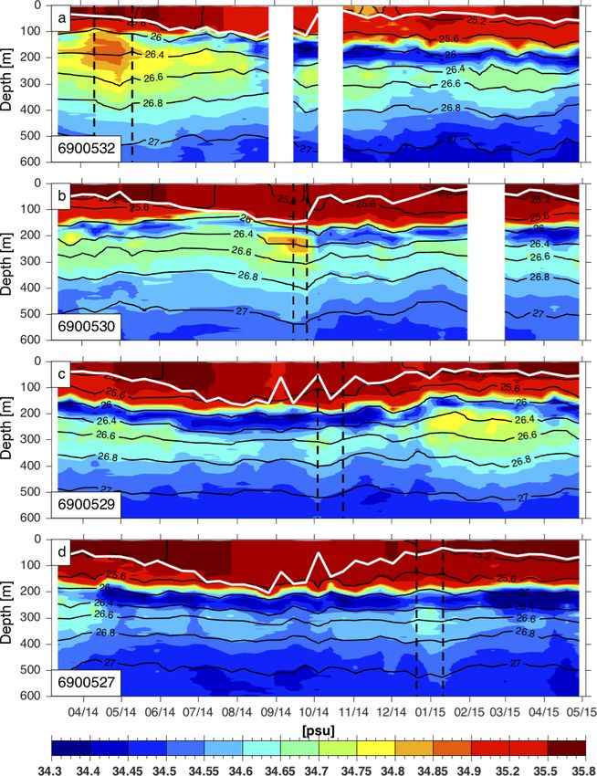
R. Czeschel et al.: Transport, properties, and life cycles of mesoscale eddies 735
ing that time span were mirrored to obtain the full coverage ETSP are covered everyday with eddies (Fig. 1a). Most of
of the MWE. the eddies are generated close to the Peruvian or Chilean
coast, where large horizontal/vertical shears exist in an oth-
3.2 Determining properties of the MWE, ACE1/2, and erwise quiescent region. In almost entire agreement with
CE conducted from satellite data Chaigneau et al. (2008), hotspot locations of eddy gener-
ation are near the coast around 10◦ S and between 16 to
The eddy shape is identified by analysing streamlines of 22◦ S (Fig. 2a, b). The four eddies (MWE, CE, ACE1, and
the SLA-derived geostrophic flow around an eddy centre ACE1) described in detail below originate from the latter re-
(high/low SLA). Often the eddy boundary is defined as the gion. After their generation near the coast, the anticyclonic
streamline with the strongest swirl velocity (for more in- eddies tend to propagate north-westward, whereas cyclonic
formation on such an eddy detection algorithm see Nenci- vortices migrate south-westward (e.g. Chaigneau et al., 2008)
oli et al., 2010). For comparison of our results with the re- into the open ocean. The seasonal cycle of eddy generation,
sults of Chaigneau et al. (2011) we also use the boundary based on all new eddy detections closer than 600 km off the
definition of the streamline with the strongest swirl velocity. coast, peaks in March and has its minimum in September
Note that the identified areas are irregularly circular therefore (Fig. 2c), whereas cyclonic eddies exhibit a stronger am-
the circle-equivalent area is used to estimate the eddy radius. plitude. However, both anticyclonic as well as cyclonic ed-
Due to the resolution of the SLA data, the eddy radius must dies have their seasonal peak of formation in austral sum-
be at least 45 km to unambiguously state that the identified mer/autumn (February/March) and the lowest number at the
area is a coherent mesoscale eddy and not an artificial sig- end of austral spring (September; Fig. 2d).
nal. Clearly identified individual eddies may have a smaller The full eddy generation mechanisms are complex,
radius than 45 km to get tracked. Eddies are tracked forward whereby boundary current separation due to a sharp topo-
and backward in time following the approach described by graphic bend is one important aspect of the eddy formation
Schütte et al. (2016a). To estimate the percentage of eddy (Molemaker et al., 2015; Thomsen et al., 2016). It is sug-
coverage in the ETSP, eddies are identified and tracked be- gested that anticyclones are generated due to instabilities of
tween 1993 and 2015. In the following it was counted how the Peru Chile Undercurrent (PCUC), whereas cyclonic ed-
often a grid point (0.5◦ × 0.5◦ ) was covered by an eddy dies are formed from instabilities of the equatorward surface
structure. For the identification of eddy generation areas, ev- currents (Chaigneau et al., 2013). In this context the strength
ery newly detected eddy closer than 600 km off the coast is of the PCUC is essential (Thomsen et al., 2016). Observa-
counted in 1◦ × 1◦ boxes. The sum of all these boxes is taken tions as well as models show a weak seasonal variability
to compute the seasonal cycle of eddy generation. The Argo in the PCUC off Peru which is stronger in austral summer
float profiles and the mooring time series are separated into and autumn (Thomsen et al., 2016; Chaigneau et al., 2013;
data conducted within cyclones, anticyclones, and the “sur- Penven et al., 2005) and might explain the higher number
rounding area” which is not associated with eddy-like struc- of eddy generation during this season. Other model simula-
tures also following the approach of Schütte et al. (2016a). tions have revealed a seasonal cycle in eddy flux that peaks
In addition the relative position of the mooring or Argo float in austral winter at the northern boundary of the OMZ, while
profile in relation to the eddy centre and eddy boundary could it peaks a season later at the southern boundary (Vergara et
be computed. al., 2016). The PCUC also experiences relatively strong fluc-
Furthermore, the composites of the eddy surface signa- tuations with periods of a few days to a few weeks (Huyer et
tures (SLA, SST, and Chl) consist of 150 × 150 km snap- al., 1991).
shots around the identified eddy centres. To exclude large-
scale variations, the SST data are low-pass filtered (cut-off 4.2 Eddy observations from March 2014 to April 2015
wavelength of 15◦ longitude and 5◦ latitude) and subtracted at the Stratus mooring
from the original data to preserve only the mesoscale vari-
ability (see Schütte et al., 2016a, for more details). From March 2014 to April 2015 the Stratus mooring was lo-
cated at 19◦ 370 S, 84◦ 570 W, about 1500 km offshore in the
4 Results oligotrophic open ocean. Oxygen, salinity, and meridional
velocity component time series for the upper 600 m (Fig. 3;
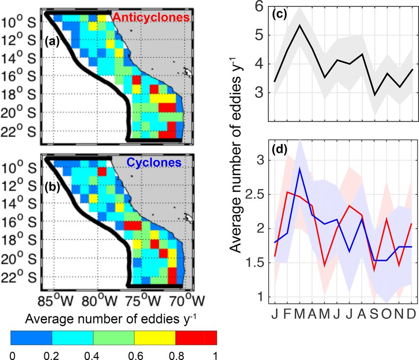
4.1 General eddy generation and its seasonal cycle in Supplement Fig. S2) record the passage of several eddies be-
the ETSP tween March 2014 and April 2015. These observations are in
agreement with the satellite data (SLA, SST, and Chl) at the
In the ETSP, 5244 eddies (49 % cyclones; 51 % anticyclones) mooring location and the 450 to 295 m geopotential anomaly
are found between January 1993 and December 2015 (re- (Fig. 3a).
quirement: having a radius between 45 and 150 km and vis- At the time of the mooring deployment on 8 March 2014
ible for more than 7 days). Both types of eddies have an an anticyclonic MWE with a radius of 43 km passed west-
average radius of about 70 km and on average 15 % of the ward with the eddy centre to the north of the mooring while a
www.ocean-sci.net/14/731/2018/ Ocean Sci., 14, 731–750, 2018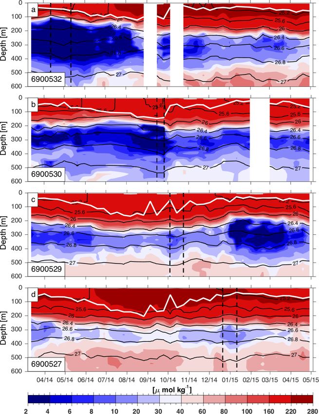
736                                                  R. Czeschel et al.: Transport, properties, and life cycles of mesoscale eddies

                                                                         lowest oxygen values of 3.8 µmol kg−1 were reached in early
                                                                         December 2014 (Fig. 3c). The massive deepening of the py-
                                                                         cnoclines is also reflected by maxima in salinity (34.69 psu)
                                                                         and temperature (10.33 ◦ C) in 350 m depth (not shown).
                                                                         The ACE2 shows high meridional velocities of more than
                                                                         5 cm s−1 in the upper 450 m depth.
                                                                             The lowest SLA and geopotential anomaly of the moor-
                                                                         ing deployment period was connected to a strong upward
                                                                         displacement of the isopycnals in February/March 2015
                                                                         (Fig. 3c). The doming of the pycnoclines from January to
                                                                         March 2015 is associated with the typical signature of cy-
                                                                         clonic eddies, which uplift colder, less saline and low-oxygen
                                                                         waters to shallower depths. Low values for oxygen, temper-
                                                                         ature, and salinity at 183 m depth of 69.1µmol kg−1 , 11.7 ◦ C
                                                                         and 34.54 psu in early February 2015 were related to a cy-
                                                                         clonic eddy (CE) with a radius of 71 km. Water properties
                                                                         of the CE may be associated with the Eastern South Pacific
                                                                         Intermediate Water which is transported by equatorward sur-
Figure 2. Number of (a) anticyclones and (b) cyclones generated in       face currents (Chaigneau et al., 2011).
1◦ × 1◦ boxes (colours) between 1993 and 2015 closer than 600 km             According to the SLA satellite maps the centre of the
off the coast (coastal region). Seasonal cycle of the number of all      MWE passed north of the mooring (Fig. 3b). The centre of
eddies (black line), anticyclones (red line), and cyclones (blue line)   the westward propagating ACE1 and the ACE2 passed the
generated in the coastal region are shown in (c) and (d).                Stratus mooring only 14 km and 17 km, respectively, south of
                                                                         it, hence the Stratus measurements were close to the centre
                                                                         of these two eddies (Fig. 3b; Supplement movie M1). How-
cyclonic eddy was located south of the mooring site (Fig. 3b;            ever, satellite data show that the mooring captured only the
Supplement movie M1). The mooring instruments recorded                   northern segment of the ACE1 (Fig. 3b), therefore the ra-
the parameter distribution at the southern rim of the MWE                dius of 28 km determined from measurements at the Stratus
revealing anomalous low oxygen of less than 10 µmol kg−1                 mooring is small in comparison to a mean radius of 40 km
and anomalous high salinity (temperature) of more than                   from satellite maps (Fig. 5a). Oxygen anomalies from Jan-
34.65 psu (10.6 ◦ C) in the eddy core in 300 m depth. It was             uary to March 2015 are related by two consecutive cyclonic
accompanied with an upward bending of isopycnals above                   eddies explaining the long-lasting and strong anomaly. The
(∼ 250 m depth) and downward bending beneath (∼ 350 m                    first eddy (CE) passed the mooring 43 km north of it and then
depth) the eddy core (Fig. 3c, d), which is typical for a mode-          merged with a second cyclonic eddy and passed to the south
water eddy in contrast to anticyclonic and cyclonic eddies. In           of the mooring (Fig. 3b).
late March 2014 the MWE had passed the mooring.                              Therefore, eddy events lead to a strong signal in water
   A strong oxygen decrease as well as a salinity increase               mass properties up to 196 (40) µmol kg−1 in oxygen, 0.84
with a strong downward displacement of the isopycnals at                 (0.18) psu in salinity, and 6.0 (1.9) ◦ C in temperature in
mid-depth in early August 2014 was related to an anticy-                 183 m (350 m) depth. The oxygen time series at 107 m depth
clonic eddy (eddy ACE1; Fig. 3c) that passed the mooring                 (Supplement Fig. S2) does not show larger anomalies from
south of it (Fig. 3b). In the upper 250 m the oxygen con-                the mean values in March and late August, at the time the
centration increased with the maximum about 10 days later                Stratus mooring near sea surface temperature signal showed
than the oxygen minimum at 290 to 600 m depth (Supple-                   the maximum and minimum of a seasonal signal (Colbo and
ment Fig. S2). At 183 m depth, maxima in oxygen, tempera-                Weller, 2007; their Fig. 3). Hence, the maxima and minima
ture and salinity of 265 µmol kg−1 , 17.73 ◦ C, and 35.38 psu,           described above for the Stratus time series at 183 and 350 m
respectively, were reached in mid-August 2014 reflecting                 are clearly related to eddies and not related to the seasonal
the deepening of the pycnocline which brings warmer, more                signal in the upper layer of the open ocean.
saline and oxygen-rich waters to deeper levels. The ACE1
shows meridional velocities of more than 5 cm s−1 in the up-             4.3   Net transport of heat, salt, and oxygen via eddies in
per 300 m depth (Fig. 3e).                                                     the ETSP
   Another strong oxygen decrease influenced the oxygen
distribution from early November 2014 to early January                   Horizontal eddy transport can be explained by two mecha-
2015. This anticyclonic eddy (eddy ACE2) had a radius of                 nisms: (1) by eddy stirring, which occurs at the periphery of
53 km and showed the strongest downward displacement of                  the eddy (e.g. Gaube et al., 2015; Chelton et al., 2011) and
the isopycnals in the 300 to 600 m range. At 350 m depth                 (2) by eddy transport of water masses trapped in the eddy

Ocean Sci., 14, 731–750, 2018                                                                       www.ocean-sci.net/14/731/2018/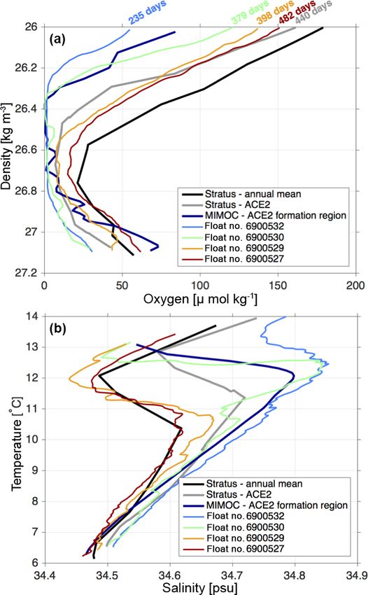
R. Czeschel et al.: Transport, properties, and life cycles of mesoscale eddies                                                            737

Figure 3. Time series for the deployment period 8 March 2014 to 25 April 2015 at the position of the Stratus mooring (19◦ 370 S, 84◦ 570 W)
for (a) weekly-delayed, high-pass filtered sea level anomaly (in cm; blue curve) and geopotential anomaly between 450 and 295 m depth
in m2 s−2 (orange curve), (c) oxygen in µmol kg−1 , (d) salinity, and (e) the meridional velocity component in cm s−1 , Hovmöller diagram
(time–latitude) at the longitude position of the Stratus mooring for (b) SLA in cm. The white curve in (e) is the mixed layer depth defined for
the depth where the potential density anomaly is 0.125 kg m−3 larger than at the surface. The black dots on the vertical line at the left mark
the depths of the used oxygen (c), conductivity (d), and velocity (e) sensors and the black contour lines are selected density contours. Black
solid (dashed) lines show the date of the passages of the anticyclonic (cyclonic) eddies.

www.ocean-sci.net/14/731/2018/                                                                             Ocean Sci., 14, 731–750, 2018
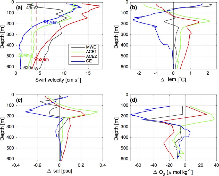
738                                                 R. Czeschel et al.: Transport, properties, and life cycles of mesoscale eddies

Figure 4. Composite of the MWE (a, e, i), ACE1 (b, f, j), ACE2 (c, g, k), and CE (d, h, l) surface signatures for SLA, SST anomaly, and
Chl. The dashed black and white line is the eddy boundary, defined as the streamline of strongest velocity. The grey line in (a) and (d) is the
position of the Stratus mooring during the eddy passage. The locations of the floats crossing the eddies are marked by coloured dots (float
#6900527 – red, #6900529 – orange, #6900530 – green, #6900532 – blue).

interior (Gaube, 2013, 2015). We are focusing on the lat-                 Typically for anticyclones, largest velocities occur in the up-
ter mechanism. The question of how much anomalous wa-                     per 250 m depth, whereas the MWE shows weak rotation
ter properties an eddy is able to trap and transport into the             in the near surface and a deeper core instead. Below 250 m
open ocean depends on the relation between swirl velocity                 depth, the swirl velocity of ACE1 is significantly weaker than
and propagation velocity. The MWE and the ACE2 have a                     the swirl velocity of ACE2. Nonetheless, due to the much
similar propagation velocity of 4.3 and 4.2 cm s−1 , respec-              slower propagation velocity of ACE1 the fluid stays trapped
tively. The CE propagates fastest (6 cm s−1 ) and the ACE1                within the eddy (U/c>1) leading to a deep vertical extent
propagates slowest (3.2 cm s−1 ) (Fig. 6a), which fits well to            of both anticyclones of 504 m (ACE1) and 523 m (ACE2) as
the mean westward propagation speed of 3–6 and 4.3 cm s−1                 described for mean anticyclones in the ETSP (Chaigneau et
estimated for eddies in the region off Peru (Chaigneau et al.,            al., 2011).
2008, 2011).                                                                 Within the eddy boundaries of the two anticyclones (ACE1
   The observed swirl velocity at the Stratus mooring is                  and ACE2), positive anomalies of temperature and salinity
in accordance with other values measured in the ETSP                      were observed between 100 and 600 m depth (Fig. 6b, c). Be-
(Chaigneau et al., 2011; Stramma et al., 2013, 2014). All                 tween 150 and 200 m depth maximum anomalies of 2.1 ◦ C
anticyclones (MWE, ACE1, and ACE2) show high rotation                     (ACE1) and 1.5 ◦ C (ACE2) in temperature and 0.35 psu
values in the upper 200 m depth with maximum velocities                   (ACE1) and 0.24 psu (ACE2) in salinity were measured
of 11, 13, and 17 cm s−1 , respectively (Fig. 6a), which is               which are significantly higher than described for the mean
between the values of mean anticyclonic eddies (9 cm s−1 ;                of a composite of anticyclones (0.8 ◦ C, 0.08 psu; Chaigneau
Chaigneau et al., 2011) and a strong relatively young anticy-             et al., 2011). Due to the uplift (depression) of isopycnals
clonic coastal mode-water eddy (35 cm s−1 ; Stramma et al.,               above (below) 200 m depth the MWE shows negative (pos-
2013). Further, the stronger swirl velocity of ACE2 agrees                itive) anomalies in temperature and salinity between 50 and
very well with an anticyclonic eddy, which passed the Stratus             200 m (below 200 m) depth, which are weak in comparison
mooring during September to December 2011 at about the                    to the other two anticyclones.
same season as for ACE2 (19 cm s−1 ; Stramma et al., 2014).

Ocean Sci., 14, 731–750, 2018                                                                           www.ocean-sci.net/14/731/2018/
R. Czeschel et al.: Transport, properties, and life cycles of mesoscale eddies                                                                                                    739

                                  (a)                        Radius = r                                             (b)      Average maximal rotation = u
                             60
                             50

                                                                                                 [m s -1 ]
                      [km]
                             40                                                                              0.2

                     [km]
                             30
                             20
                             10             1                     2   3         4
                                                                                                               0
                                  0             0.2        0.4      0.6        0.8           1                     0         0.2         0.4      0.6       0.8   1
                                                      normalized eddy lifetime

                                  (c)             Nonlinearity parameter                                            (d)               Rossby number
                              4
                                                                                                             0.5

                                                                                                   [u/fr]
                      [u/c]

                              2

                              0                                                                                0
                                  0             0.2         0.4           0.6       0.8      1                     0         0.2         0.4      0.6       0.8   1

                                      (e)                  Centred SLA                                                 (f)              Centred SST
                             10                                                                              0.1

                              5                                                                                0
                     [cm]

                                                                                                   [°C]
                              0                                                                              -0.1

                             -5                                                                              -0.2
                                  0             0.2        0.4      0.6        0.8           1                      0        0.2        0.4      0.6        0.8   1
                                                      normalized eddy lifetime                                                     normalized eddy lifetime
                                                                                     Normalized eddy lifetime

Figure 5. (a) Eddy radius, (b) averaged maximum rotation velocity, (c) nonlinearity parameter (U/c), (d) Rossby number (U/f r), (e) centred
SLA, and (f) centred SST anomaly against normalized eddy lifetime of the ACE1 (green), ACE2 (red), CE (blue), and MWE (black). The
coloured solid lines mark the passage at the Stratus mooring of the corresponding eddies. The residence times of the four floats trapped in
the ACE2 are marked by red dashed lines in (a).

Figure 6. (a) Swirl velocity vs. depth (solid lines), propagation velocity (dashed lines), and vertical extent of the trapped fluid (circles) of
three anticyclonic eddies (MWE: grey, ACE1: green, ACE2: red) and a cyclonic eddy (CE: blue). Profiles of anomalies of (b) temperature,
(c) salinity, and (d) oxygen (µmol kg−1 ) calculated as the difference between the core of MWE (grey), ACE1 (green), ACE2 (red), and CE
(blue) as well as the 1-year mean of the Stratus mooring (10 April 2014–9 April 2015).

www.ocean-sci.net/14/731/2018/                                                                                                                           Ocean Sci., 14, 731–750, 2018
740 R. Czeschel et al.: Transport, properties, and life cycles of mesoscale eddies Oxygen shows a mainly negative anomaly below 100, 220, The cyclonic eddy in March 2015 (CE) has maximum ve- and 280 m depth respectively within the anticyclones MWE, locities of 14 cm s−1 in 50 m depth (Fig. 6a). Due to the high AC1, and AC2. Both the MWE and the ACE2 are having translation speed of the CE, the vertical extent of 176 m depth their largest negative anomalies in 250 m depth and a second is much shallower than the vertical extent of the anticyclones, minimum in 450 m depth, which is just above and below the which is consistent with the mean cyclones (Chaigneau et core of the OMZ indicating the transport of low oxygenated al., 2011). The mean temperature shows a pronounced neg- water masses from a region with a larger vertical expansion ative anomaly within the eddy boundaries between 70 and of the OMZ (Fig. 6d). In the core depth of the OMZ at 350 m 430 m depth with a maximum anomaly of −2.3 ◦ C in 160 m depth, only weak negative oxygen anomalies are possible as (Fig. 6b) resulting in a negative AHA of −8.9 × 10¹⁸ J. The the oxygen content is already low, but still the passage of the salinity is negative between 40 and 220 m depth with a maxi- stronger anticyclone ACE2 results in an oxygen decrease by mum anomaly of −0.32 psu in 160 m depth (Fig. 6c). This re- 14 µmol kg−1 . sults in an extremely large negative ASA of −41.5×10¹⁰ kg. Water mass anomalies within the MWE lead to avail- Oxygen shows a strong negative anomaly in the upper 320 m able heat, salt, and oxygen anomalies (AHA, ASA, AOA) having a maximum anomaly of −69 µmol kg−1 in 180 m of 1.0×10¹⁸ J, −3.1×10¹⁰ kg, and −3.5×10¹⁶ µmol. These depth (Fig. 6d) due to the uplift of the main thermocline lead- values are about 5 times smaller in comparison to a mode- ing to a negative AOA of −6.5 × 10¹⁶ µmol for the 107 to water eddy that was also measured at the Stratus mooring 176 m depth layer. Although the volume of the CE is in good in February/March 2012 (Stramma et al., 2014; Table 1). agreement with the mean values of Chaigneau et al. (2011), ASA is even negative in 2015 due to the strong doming the estimated AHA and ASA are much higher (Table 1), in the upper 200 m. As both mode-water eddies have about which is likely due to strong seasonal variations during the the same propagation speed and volume, the differences generation of the CE. The CE is formed in austral winter off in water mass properties point towards seasonal or inter- Peru when coastal alongshore winds intensify leading to an annual variations of the water mass characteristics during enhanced upwelling of cold and nutrient-rich and oxygen- their formation. The MWE is generated in February, when poor water due to high biological production. Additionally, upwelling-favourable alongshore winds weaken and SST in- equatorward surface currents, which transport the relatively creases (Gutiérrez et al., 2011), whereas the mode-water cold and fresh Eastern South Pacific Intermediate Water, are eddy observed by Stramma et al. (2014) is generated in April, strongest during austral winter (Gunther, 1936). when the PCUC, which transports oxygen-deficient ESSW Fluxes of mass, heat, salinity, and oxygen are estimated (Hormazabal et al., 2013), has its poleward maximum (Shaf- from the volume, AHA, ASA, and AOA (Table 1) for the fer et al., 1999; Penven et al., 2005; Chaigneau et al., 2013). period in which the MWE, ACE2, and CE cross the 85◦ W In addition, the MWE passed to the north of the Stratus moor- longitude at the Stratus mooring. The ratio of the heat fluxes ing during its deployment, hence the method to define the of the three different eddies mirror the differences between fully MWE parameter might lead to higher deviations to the volume, AHA, ASA, and AOA of the respective eddies be- real eddy parameters. cause of the similar duration of the passages of the eddies. The volume of ACE2 (4.6 × 10¹² m3 ) is in agreement with Transports of mass anomaly for the CE, ACE2, and MWE the mean anticyclones (Chaigneau et al., 2011) and the open- are again similar and range between 1.1 Sv for the CE and ocean anticyclone (Stramma et al., 2013) but 3 times larger 1.8 Sv for ACE2 (Table 2). Due to the local conditions and than the weaker ACE1, which is partly due to the underesti- different water masses during its formation, the CE shows mated radius (Table 1). The AHA, ASA, and AOA of ACE2 a strong negative transport of heat (−3.8 × 10¹² W) and salt are 8.1 × 10¹⁸ J, 25.2 × 10¹⁰ kg, and −3.6 × 10¹⁶ µmol and (−17.5 × 10⁴ kg s−1 ) across the mooring, whereas the ACE2 therefore far greater than the AHA, ASA, and AOA of ACE1 transports the highest positive amount of heat (3.2 × 10¹² W) (1.8 × 10¹⁸ J, 5.5 × 10¹⁰ kg, −0.02 × 10¹⁶ µmol). The weak and salt (10.0 × 10⁴ kg s−1 ) per year. Whereas the transport negative AOA of ACE1 result from the strong and positive of heat and salt of the MWE is relatively small in compari- oxygen anomaly in the upper 280 m depth in comparison to son to the CE and ACE2, the transport of low oxygen water the background water mass. Strong differences between the of −1.8 × 10¹⁰ µmol s−1 is in the same range as the CE and results for ACE1 and ACE2 are of course due to the higher ACE2 due to a thick lens of low-oxygen water within the volume of the ACE2 but might also reflect the conditions at MWE. different seasons during the formation of the eddies leading Available anomalies of heat, salt, and oxygen of cyclonic to varying water mass properties. ACE1 (ACE2) is generated and anticyclonic eddies gained from the Stratus mooring and in austral summer (winter) when upwelling-favourable winds from the literature (Table 1) are now used to estimate the rel- weaken (strengthen). Estimations of AHA and ASA within ative contribution of long-lived eddies to fluxes of mass, heat, ACE2 match the mean values of Chaigneau et al. (2011). In salt, and oxygen in an offshore area of the ETSP. The mean comparison to the open-ocean eddy (Stramma et al., 2013) heat (in W), salt (in kg s−1 ), and oxygen transport (µmol s−1 ) the AHA of the ACE2 is twice as high, but the AOA is only are calculated by multiplying the amount of AHA, ASA, and half as much (Table 1). AOA of the composite eddies with the number of eddies dis- Ocean Sci., 14, 731–750, 2018 www.ocean-sci.net/14/731/2018/
R. Czeschel et al.: Transport, properties, and life cycles of mesoscale eddies                                                               741

Table 1. Properties and available heat, salt, and oxygen anomalies (AHA, ASA, AOA) with error bars of one mode-water eddy (MWE),
two anticyclones (AE1 and AE2), and one cyclonic eddy (CE) measured at the Stratus mooring in 2014/2015 within the vertical layer of the
coherent structure in comparison to measurements in February/March 2012 (Stramma et al., 2014; STR14, mode-water eddy) at the Stratus
mooring, at 16◦ 450 S, 83◦ 500 W in November 2012 (Stramma et al., 2013; STR13, anticyclone) and mean values for 10–20◦ S relative to a
mean climatology (Chaigneau et al., 2011; CH11, anticyclones and cyclones). Based on instruments available, the vertical extent for heat
and salt computations (TS) and oxygen (OX) differs. It is important to note that the radius of the ACE1 might be underestimated.

                                 Mode-water eddies                          Anticyclones                                    Cyclones
                           MWE              STR14    ACE1             ACE2                 STR13       CH11        CE             CH11
    Lifetime (days)        768              315      624              650                                          229
    Propagation            4.3              4        3.2              4.2                  4.8         4.3         6              4.3
    (cm s−1 )
    Radius (km)            43 ± 2           38       (28 ± 2)         53 ± 4               49          58          71 ± 1         62
    Vertical extent   TS   43–620           45–600   13–504           13–523               0–600       0–450       13–176         0–200
    (m)               OX   107–600                   107–504          107–523                                      107–176
    Volume            TS   3.4 ± 0.4        2.5      (1.3 ± 0.2)      4.6 ± 0.4            4.7         4.9         2.7 ± 0.1      2.6
    (×1012 m3 )       OX   2.9 ± 0.4                 (1 ± 0.1)        3.8 ± 0.4                                    1.1 ± 0
    AHA                    1.0 ± 0.2        5.8      (1.8 ± 0.8)      8.1 ± 2.1            3.7         6.5         −8.9 ± 0.7     −5.9
    (×1018 J)
    ASA                    −3.1 ± 0.4       19.3     (5.5 ± 1.0)      25.2 ± 3.7           18.7        17.4        −41.5±0.1      −14.7
    (×1010 kg)
    AOA                    −3.5 ± 1.2       −10.5    (−0.02 ± 0.32)   −3.6 ± 1.9           −7.6        –           −6.5 ± 0.5     –
    (×1016 µmol)

sipating per year in an offshore area (corresponding to a flux        Table 2. Mass, heat, salt, and oxygen transport with error bars of
divergence). We define an area over a north–south direction           MWE, ACE2, CE across 85◦ W of the Stratus mooring 2014/2015.
from 10 to 24◦ S. The transition area is bordered in the east
by a line running parallel to the Peruvian and Chilean coast                                           MWE              ACE2               CE
at a distance of 6◦ and in the west by the 90◦ W longitude              Mass transport              1.7 ± 0.1          1.8 ± 0          1.1 ± 0
corresponding to a size of ∼ 1.7 × 10⁶ km2 . Based on aver-             (Sv)
aged satellite measurements, 58.6 eddies of all eddies that
are generated off the coast (Fig. 2) reach the offshore area            Heat transport              0.5 ± 0.1      3.2 ± 0.6      −3.8 ± 0.3
per year from which 28.9 are cyclones and 29.7 are anticy-              (×1012 W)
clones. Also, 2.1 cyclones and 0.7 anticyclones and mode-               Salt transport             −1.6 ± 0.3     10.0 ± 0.8     −17.5 ± 0.3
water eddies propagate into the area west of the 90◦ W lon-             (×104 kg s−1 )
gitude meaning that 26.8 of the cyclones and 29 of the anti-
                                                                        Oxygen transport           −1.8 ± 0.4    −1.4 ± 0.7       −2.7 ± 0.1
cyclones and mode-water eddies have dissipated and there-
                                                                        (×1010 µmol s−1 )
fore transported a certain amount of heat, salt, and oxygen
into the offshore zone. Based on the mean of AHA, ASA,
and AOA for the composite eddies, the mean transport of
heat (salt, oxygen) per year from the coastal region into the         types of eddies show negative oxygen fluxes in the layer
transition zone is −6.4 × 10¹² W (−2.4 × 10⁵ kg s−1 , −5.7 ×          defined as the depth of the coherent structure of the eddy
1010 µmol kg−1 s−1 ) for cyclones and 4.7 × 10¹² W (1.5 ×             (Table 1) meaning that anticyclones and cyclones transport
105 kg s−1 , −5.9 × 10¹⁰ µmol kg−1 s−1 ) for anticyclones and         less oxygenated water into the upper and mid-depth open
mode-water eddies in agreement with estimates for transport           ocean and therefore have an impact on the balance and size
anomalies of heat and salt in this region by Chaigneau et             of the OMZ in the ETSP, which is also confirmed by models
al. (2011).                                                           (Frenger et al., 2018).
   Heat and especially salt fluxes across the Stratus mooring
as well as for the ETSP reveal an imbalance between anti-             4.4      Properties of the observed eddies MWE, ACE1/2,
cyclones and cyclones which are due to a higher transport                      and CE during their lifetime
of anomalous cold and fresh water within cyclones from the
coast off Peru and Chile into the upper open ocean. Both              With the help of satellite data the four eddies (MWE,
                                                                      ACE1/2, and CE) could be identified and followed from ar-

www.ocean-sci.net/14/731/2018/                                                                               Ocean Sci., 14, 731–750, 2018
742 R. Czeschel et al.: Transport, properties, and life cycles of mesoscale eddies eas near the Peruvian and off the Chilean coast to the ar- during their mid-age (MWE and ACE2) and during the end eas of dissipation westwards of the Stratus mooring in the of their lifetime (ACE1 and CE). The anticyclones ACE1/2 open ocean. The trajectories of the three anticyclonic ed- have their maximum radius during the last third of their life- dies (MWE, ACE1/2) were extrapolated to the formation re- time, whereas the development of the radius of the MWE is gions near the coast between 20 and 23◦ S (Fig. 1). The CE symmetric and the radius of the CE increases during the first formed during end of July 2014 off the Peruvian coast dur- third of its lifetime (Fig. 5a). Note the decreasing maximum ing the winter season when upwelling is usually strong and rotation velocity of the ACE2 during the second half of its decayed in mid-March 2015 after propagating 1200 km in lifetime (Fig. 5b). more than 7 months. Both the MWE and the ACE1 started off Water mass anomalies can only be preserved within an the Chilean coast during the end of the summer season with eddy if the feature is nonlinear and maintains its coherent usually low upwelling. The MWE can be followed for about structure. During their full lifetime, the nonlinear parame- 2 years till March 2015 propagating 2880 km. The ACE1 is ter U/c>1 for all eddies and confirms the coherent feature tracked for 620 days until it decayed at the end of Novem- (Fig. 5c). Nonetheless, significant variations in the nonlin- ber 2014, after propagating 1750 km. The ACE2, which was ear parameter U/c determined at the surface might indicate generated during the upwelling season at the end of winter changes in the volume of the eddies, which can be influenced in September 2013 and decayed in June 2015, propagated by friction, stratification, fluctuations of the mean flow, or the westward for 2350 km in 650 days. collapse with other eddies. Maps of SLA show a permanent As expected from the polarity depending meridional de- change of the radius due to an irregular and varying shape flection of all eddies (anticyclones – equatorward, cyclones – and the merging with other eddies (Supplement: movie M1), poleward), the individual pathways of the ACE1 and ACE2 which makes it sometimes difficult to track an eddy during its also show a north-westward direction whereas the CE mi- whole lifetime. Fluctuations are also produced by the coarse grates more south-westwards (Fig. 1a). Note that the MWE resolution of the satellite data (0.25◦ × 0.25◦ ) and the merg- shows no clear meridional deflection on the way to the west. ing algorithms used by AVISO. However, the MWE and CE Anticyclonic eddies (MWE, ACE1/2) are associated with show stronger fluctuations of the nonlinear parameter than a positive SLA, wherein ACE2 shows the strongest mean el- the ACE1/2, which probably mirrors the higher variability evation of all anticyclonic eddies of 8 cm (Fig. 4c) and cy- in the swirl velocity of both eddy types (Fig. 5b). Nonethe- clonic eddies are identified by a negative SLA, wherein the less, the nonlinear parameter U/c is always higher than 1 and CE shows a mean minimum SLA of −2 cm in the centre of therefore indicates a trapped volume despite strong fluctua- the eddy (Fig. 4d). Nevertheless, the CE showed the largest tions at the surface. The small variations in the eddy proper- SLA differences at the Stratus mooring (Fig. 3a). In general, ties of the ACE2 (Fig. 5a–e) suggest a relatively stable struc- mode-water eddies are difficult to detect by satellite altimetry ture. due to a relatively weak velocity near the surface (Fig. 6a), All eddies indicate a Rossby number Ro
R. Czeschel et al.: Transport, properties, and life cycles of mesoscale eddies                                                          743

Figure 7. Distribution of oxygen (in µmol kg−1 , coloured) and density (black lines) vs. time in the upper 600 m depth of floats 6900532 (a),
6900530 (b), 6900529 (c), and 6900527 (d) which have been trapped within the ACE2 at different stages. The residence time in ACE2 of
the floats in April/May 2014, September 2014, October 2014, and December 2014/January 2015 is marked by dashed black lines. The white
curve is the mixed layer depth defined for the depth where the potential density anomaly is 0.125 kg m−3 larger than at the surface.

2015. During this period, four floats (Fig. 7) were captured             incides with the water mass of the likely formation re-
within the ACE2 during its westward propagation at dif-                  gion of the ACE2 obtained from the monthly isopycnal and
ferent times providing information about different stages of             mixed-layer ocean climatology (MIMOC; Schmidtko et al.,
the eddy. The first float (#6900532) was trapped in the pe-              2013; Fig. 9a, b) reflecting the characteristics of the oxygen-
riod from mid-April to mid-May 2014 at 19.9◦ S, 77.1◦ W                  depleted ESSW. The ESSW is carried poleward by the sec-
(Supplement: movie M1). The eddy shows the core at about                 ondary southern subsurface countercurrent (Montes et al.,
isopycnal 26.4 kg m−3 (∼ 180 m depth) with extremely low                 2014), feeds the subsurface PCUC (Hormazabal et al., 2013),
oxygen of less than 4 µmol kg−1 between 150 and 400 m                    and is then transported along the Peruvian and Chilean coast
depth (Fig. 7a) and enhanced salinity of more than 34.8 psu              where anticyclonic eddies are likely generated (Chaigneau et
in the upper 240 m depth (Fig. 8a). The warm, salty, and                 al., 2011).
oxygen-depleted water mass of the core of the ACE2 co-

www.ocean-sci.net/14/731/2018/                                                                            Ocean Sci., 14, 731–750, 2018
744                                                  R. Czeschel et al.: Transport, properties, and life cycles of mesoscale eddies

Figure 8. Same as Fig. 7 but for salinity distribution.

   In September 2014, about 4 months later and more than 6◦            about σθ = 26.0 kg m−3 . This density level corresponds to a
further west at 19.4◦ S, 83.4◦ W a second float (#6900530)             depth between 100 and 170 m, where a high swirl velocity
was trapped in the same eddy ACE2 (Supplement: movie                   exists within the ACE2 (Fig. 6a), which is essential to keep
M1). The core was still located at isopycnal 26.4 kg m−3               up the coherent structure.
(∼ 230 m depth) showing minimum oxygen values of less                     Shortly after, in October 2014, a third float (#6900529)
than 4 µmol kg−1 (Fig. 7b) and maximum salinity of more                stayed in the ACE2 at about 20.4◦ S, 82.8◦ W. The
than 34.8 psu (Fig. 8b) between 200 and 280 m depth. How-              strongest water property anomaly is now located at isopy-
ever, the vertical extent of anomalously high salinity and             cnal 26.6 kg m−3 (∼ 310 m depth) showing minimum oxy-
anomalously low oxygen has decreased (Fig. 9a, b) which                gen of less than 8 µmol kg−1 (Fig. 7c). The salinity
is likely due to lateral mixing. Mixing mostly takes place             anomaly transported within the eddy has declined further
above the core of the eddy between the density layers                  to about 34.65 psu (Fig. 8c). The development of the wa-
σθ = 25.7 and σθ = 26.3 kg m−3 (Supplement Fig. S3) with               ter mass properties within the eddy points towards mixing
largest changes in oxygen (0.5 µmol kg−1 day−1 ), tempera-             along density surfaces between σθ = 26.0 kg m−3 (∼ 190 m)
ture (−0.007 ◦ C day−1 ), and salinity (−0.002 psu day−1 ) at          and σθ = 26.5 kg m−3 (280 m). The changes are strongest

Ocean Sci., 14, 731–750, 2018                                                                     www.ocean-sci.net/14/731/2018/
R. Czeschel et al.: Transport, properties, and life cycles of mesoscale eddies                                                   745

                                                                      (Fig. 9b), the oxygen anomaly transported in the core agrees
                                                                      well (Fig. 9a).
                                                                         After the ACE2 has passed the Stratus mooring in Novem-
                                                                      ber 2014, the last of the four floats (#6900527) was trapped
                                                                      at the southern rim of the eddy (Fig. 4c) from December
                                                                      2014 to January 2015 at about 20.4◦ S, 86.4◦ W. The eddy
                                                                      core is still clearly visible, although water mass proper-
                                                                      ties within the core of the ACE2 has further changed (oxy-
                                                                      gen >10 µmol kg−1 , Fig. 7d) and the vertical extent of the
                                                                      eddy has declined. Mixing of slightly oxygen-richer water
                                                                      can be observed over the whole water column (Supplement
                                                                      Fig. S3a), whereas warmer and more saline water is entrained
                                                                      in the upper part of the eddy (σθ >26.3 kg m−3 ∼       = 240 m
                                                                      depth) and colder and fresher water below. These changes
                                                                      might also be due to the location of the float outside the eddy
                                                                      boundary.

                                                                      5   Discussion and outlook

                                                                      The ETSP is known for its high eddy frequency (Chaigneau
                                                                      et al., 2008). There is still limited knowledge in this region
                                                                      about the dynamics of eddies especially on their effective
                                                                      transport and their dissipation. In this study the activity of
                                                                      three different types of eddies (mode water, anticyclonic, and
                                                                      cyclonic eddy) during their westward propagation was inves-
                                                                      tigated from the formation area in the upwelling area off Peru
                                                                      and Chile into the open ocean. The focus was on the devel-
                                                                      opment of the eddies, seasonal conditions during their for-
                                                                      mation, their life cycles and fluxes, and the change of water
                                                                      mass properties transported within the isolated eddies using
                                                                      a broad range of observational data such as SLA, SST, and
                                                                      Chl from satellites as well as hydrographic data and oxygen
                                                                      from the Stratus mooring and from Argo floats.
Figure 9. Profiles of (a) oxygen vs. density and (b) temperature–
                                                                         Available heat, salt, and oxygen anomalies could be com-
salinity diagrams at the Stratus mooring (19◦ 370 S, 84◦ 570 W) for
a 1-year mean (10 April 2014 to 9 April 2015; black) and during       puted for the investigated eddies. Generally, heat and salt
the passage of the ACE2 in November 2014 (grey line), from the        anomalies transported within eddies are positive for anti-
estimated formation region at 23◦ S, 71◦ W from the MIMOC cli-        cyclones and negative for cyclones and might be compen-
matology (dark blue) and from data of four floats (69005-27, -29,     sated for as they are of about the same amount (Chaigneau
-30, and -32) trapped in the ACE2 (for coloured lines see legend).    et al., 2011). In this study the negative and positive heat
The age of the ACE2 in days during the respective measurement is      anomalies of the CE (−8.9×10¹⁸ J), ACE2 (8.1×10¹⁸ J), and
indicated in the upper panel. The age of the ACE2 (in days) at the    MWE (1.0 × 10¹⁸ J) almost balance each other. In contrast,
time of the respective float measurements is marked in (a).           the sum of negative and positive salt anomalies transported
                                                                      within the CE (−41.5×10¹⁰ kg), ACE2 (25.2×10¹⁰ kg), and
                                                                      MWE (−3.1 × 10¹⁰ kg) is unbalanced. The AOA is nega-
above the core of the eddy at about σθ = 26.3 kg m−3                  tive for all types of eddies (MWE: −3.5 × 10¹⁶ µmol; ACE2:
(∼ 205 to 240 m) showing the mixing of oxygen-rich                    −3.6×10¹⁶ µmol; CE: −6.5×10¹⁶ µmol), whereby the trans-
(2.8 µmol kg−1 day−1 ), colder (−0.07 ◦ C day−1 ) and fresher         port of oxygen-poor water from the upwelling region into
water (−0.017 psu day−1 ) into the ACE2 (Supplement                   the open ocean is more surface intensified due to the shal-
Fig. S3).                                                             low structure of the cyclonic eddies. A mode-water eddy ob-
   Decreased anomalies might also be related to the fact that         served by Stramma et al. (2014) was generated in year 2011,
the float did not capture the eddy centre as it was located in        which is considered as a La Niña period, when generally
the south-east rim of the eddy (Fig. 4c). Whereas the salin-          lower oxygen and higher salinity values exist in the upper
ity measurements of the float differ from those of the Stra-          100 m depth (Stramma et al., 2016) leading to higher anoma-
tus measurements obtained during the passage of the ACE2              lies of salt and oxygen of the mode-water eddy observed by

www.ocean-sci.net/14/731/2018/                                                                      Ocean Sci., 14, 731–750, 2018
746 R. Czeschel et al.: Transport, properties, and life cycles of mesoscale eddies
Stramma et al. (2014) in comparison to the actual MWE. and shaping the OMZ confirmed by model studies (Frenger
Therefore, seasonal variability such as fluctuation of along- et al., 2018).
shore upwelling-favourable winds off Peru and Chile as well Thus, the variability of eddy generation on different
as interannual variability such as El Niño or La Niña have an timescales might be an important factor for the variability
impact on the water mass properties trapped and transported in the OMZ. Eddy generation off the coast between 8 and
within eddies from the coast of Peru and Chile into the open 24◦ S peak in austral summer/spring, which agrees with the
ocean reflecting the high variability of AHA and ASA. strengthening of the PCUC and the possible mechanism of
For the Atlantic Ocean the low-oxygen eddy cores have the generation of eddies due to instabilities. However, this is
been attributed to high productivity in the surface (Schütte not in agreement with model simulations showing an eddy-
et al., 2016b), enhanced respiration of sinking organic ma- induced offshore transport off Peru that peaks in austral
terial at subsurface depth (Fiedler et al., 2016), and a strong spring (winter) at the southern (northern) boundary of the
isolation of the eddy core (Karstensen et al., 2017). An anti- OMZ (Vergara et al., 2016). As the PCUC also shows strong
cyclonic mode-water eddy observed in the Pacific at the Stra- fluctuations lasting a few days up to a few weeks (Huyer et
tus mooring in February/March 2012 indicated high primary al., 1991) it might be difficult to determine a seasonal di-
production just below the mixed layer (Stramma et al., 2014). mension between the PCUC and the rate of eddy formation.
According to a global investigation of Argo floats, the eastern El Niño (La Niña) events deepen (shoal) the thermocline
South Pacific off Peru and Chile seems to have the highest and intensify (weaken) the PCUC (e.g. Montes et al., 2011;
amount of MWEs, which are also deep reaching compared Combes et al., 2015). Intraseasonal and interannual variabil-
to other regions (Zhang et al., 2017; their Fig. 2). Neverthe- ity is another factor modulating the strength of the PCUC off
less, in the mooring deployment period 2014/2015 only one Chile and therefore the formation rate of anticyclonic eddies
MWE crossed to the north of the mooring and the results (Shaffer et al., 1999).
have to be regarded with caution. Even though the AHA and In this study the development of isolated water mass prop-
ASA of the MWE are small in comparison to both the an- erties was investigated on the basis of four floats trapped
ticyclonic eddies and the cyclonic eddy the transport of low within an anticyclonic eddy indicating lateral mixing of all
oxygen water is in the same range as the other eddies due to water properties (oxygen, temperature, and salinity). The wa-
the typical thick lens of low oxygen water within mode-water ter mass within the core of the ACE2 shows the typical char-
eddies. acteristics of the salty and oxygen-depleted ESSW. The mix-
From a combination of satellite data and Argo profiles, ing is strongest between the seasonal thermocline and the
long-lived eddies (lifetime longer than 30 days) in the core of the eddy at about σθ = 26.3 kg m−3 (∼ 205 to 240 m
Peru-Chile upwelling system (55 % of the sampled anticy- depth) and takes place during the first half of the lifetime of
clonic eddies) had subsurface-intensified maximum temper- the eddy. During this period the variability in the amplitude
ature and salinity anomalies below the seasonal pycnocline, of the ACE2 is negligibly small, which might be due to the
whereas 88 % of the cyclonic eddies are surface intensi- coarse resolution of the satellite data. The radius increases
fied (Pegliasco et al., 2015). The 55 % subsurface-intensified up to 50 km with a nearly consistent rotation velocity at the
anticyclonic eddies represent mode-water eddies while the same time (Fig. 5a, b). During the second half of the lifetime
45 % surface intensified anticyclones are “regular” anticy- the radius of the ACE2 slightly increases but the maximum
clonic eddies. Observations and model results for the Cal- rotation velocity and therefore the nonlinear parameter de-
ifornia Current system showed a good agreement between creases (Fig. 5c) until the decay of the ACE2. Stronger mix-
observed and modelled eddy structures (Kurian et al., 2011). ing during the first half of the eddy lifetime could be related
Satellite-based estimate of the surface-layer eddy heat flux to a stronger wind curl near the coast in comparison to the
divergence, while large in coastal regions, is small when open ocean (Albert et al., 2010, their Fig. 1b). However, as
averaged over the south-east Pacific Ocean, suggesting that the changes might also be due to the fact that the floats might
eddies do not substantially contribute to cooling the sur- be located at different positions within the eddy or near the
face layer in this region (Holte et al., 2013). In this study, outer edge these results should be regarded with caution. Of-
the release of fluxes of heat (cyclones: −6.4 × 10¹² W; an- ten floats are carried with the eddies near the outer edge of
ticyclones: 4.7 × 10¹² W) and salt (−2.4 × 10⁵ kg s−1 ; 1.5 × the eddy, avoid the core of eddies, and hence underestimate
105 kg s−1 ) estimated from long-lived eddies dissipating in the strength of eddies. Especially floats with a parking depth
the ETSP confirms the discrepancy between different types at 400 m stay near the edge of eddies and shift between cy-
of eddies leading to a net transport of colder and fresher water clonic and anticyclonic features. If located in the ETSP at
from the formation regions off Peru and Chile into the open southern boundaries of anticyclones or northern boundaries
ocean. In contrast, all three types of eddies show a negative of cyclones the floats move eastward while floats at north-
oxygen flux of −5.7 × 10¹¹ µmol kg−1 s−1 for cyclones and ern boundaries of anticyclones or southern boundaries of cy-
−5.9 × 10¹⁰ µmol kg−1 s−1 for anticyclones and mode-water clones move westward (see Supplement movie M1).
eddies pointing towards an active role of eddies in balancing Eddies play an important role in the weak circulation re-
gion of the ETSP. Regarding the mean flow in the ETSP at
Ocean Sci., 14, 731–750, 2018 www.ocean-sci.net/14/731/2018/You can also read