Effect of stress history on sediment transport and channel adjustment in graded gravel-bed rivers
←
→
Page content transcription
If your browser does not render page correctly, please read the page content below
Earth Surf. Dynam., 9, 333–350, 2021
https://doi.org/10.5194/esurf-9-333-2021
© Author(s) 2021. This work is distributed under
the Creative Commons Attribution 4.0 License.

               Effect of stress history on sediment transport and
                channel adjustment in graded gravel-bed rivers
                         Chenge An1,2 , Marwan A. Hassan2 , Carles Ferrer-Boix3 , and Xudong Fu1
               1 Department of Hydraulic Engineering, State Key Laboratory of Hydroscience and Engineering,
                                             Tsinghua University, Beijing, China
                   2 Department of Geography, The University of British Columbia, Vancouver, BC, Canada
                           3 Serra Húnter Fellow, Department of Graphic and Design Engineering,

                                     Technical University of Catalonia, Barcelona, Spain
                                     Correspondence: Xudong Fu (xdfu@tsinghua.edu.cn)

                                   Received: 5 August 2020 – Discussion started: 8 September 2020
                           Revised: 13 December 2020 – Accepted: 9 March 2021 – Published: 21 April 2021

       Abstract. With the increasing attention on environmental flow management for the maintenance of habitat
       diversity and ecosystem health of mountain gravel-bed rivers, much interest has been paid to how inter-flood low
       flow can affect gravel-bed river morphodynamics during subsequent flood events. Previous research has found
       that antecedent conditioning flow can lead to an increase in critical shear stress and a reduction in sediment
       transport rate during a subsequent flood. However, how long this effect can last during the flood event has
       not been fully discussed. In this paper, a series of flume experiments with various durations of conditioning
       flow are presented to study this problem. Results show that channel morphology adjusts significantly within
       the first 15 min of the conditioning flow but becomes rather stable during the remainder of the conditioning
       flow. The implementation of conditioning flow can indeed lead to a reduction of sediment transport rate during
       the subsequent hydrograph, but such an effect is limited to within a relatively short time at the beginning of
       the hydrograph. This indicates that bed reorganization during the conditioning phase, which induces the stress
       history effect, is likely to be erased with increasing intensity of flow and sediment transport during the subsequent
       flood event.

1   Introduction                                                    were mostly developed for lowland streams with continuous
                                                                    sediment supply and an average flow regime, which do not
Prediction of sediment transport is of vital importance be-         apply to mountain streams (Gomez and Church, 1989; Rick-
cause it is related to many aspects of river dynamics and           enmann, 2001; Schneider et al., 2015).
management, including river morphodynamics modeling                    For example, the hydrograph of mountain gravel-bed
(Parker, 2004), river restoration (Chin et al., 2009), aquatic      rivers is often characterized by large fluctuations of flow dis-
habitats (Montgomery et al., 1996), natural hazard plan-            charge, including both short-term flash flood and long-term
ning (Marston, 2008), bedrock erosion (Sklar and Dietrich,          inter-flood low flow (Powell et al., 1999). However, research
2004), and landscape evolution (Howard, 1994). In gravel-           on the morphodynamics of mountain rivers often focuses on
bed rivers, sediment transport is controlled by flow magni-         the effects of floods (or constant high flow) and neglects the
tude and flashiness, sediment supply, bed surface structures,       role of inter-flood low flow, with the consideration that most
channel morphology, and the grain size distribution (GSD)           sediment transport and morphological adjustments of moun-
of sediment (Montgomery and Buffington, 1997; Masteller             tain rivers occur during relatively high flows (Klingeman and
et al., 2019). Therefore, prediction of sediment transport in       Emmett, 1982; Paola et al., 1992).
mountain rivers still remains difficult despite the large body         Reid and colleagues (Reid and Frostick, 1984; Reid et al.,
of existing theories. This is due to the fact that these theories   1985) studied the effects of inter-flood low flow on subse-

Published by Copernicus Publications on behalf of the European Geosciences Union.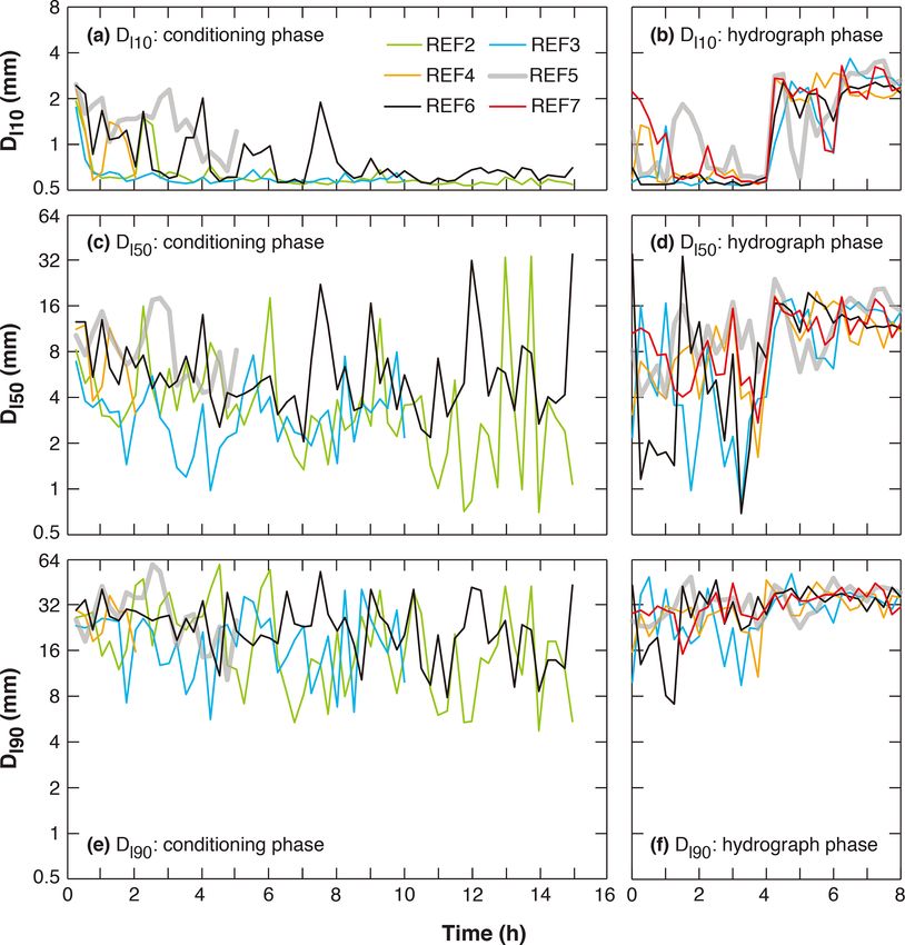
334                                      C. An et al.: Effect of stress history on sediment transport and channel adjustment

quent sediment transport in Turkey Brook, England. They              Because of the above-mentioned research, existing sedi-
found that bed load transport rates were reduced during rel-      ment transport formulae for gravel-bed rivers (e.g., Meyer-
atively isolated flood events (e.g., events separated by long     Peter and Müller, 1948; Parker, 1990; Wilcock and Crowe,
time intervals) compared to those that were closely spaced,       2003; Wong and Parker, 2006) are regarded as inaccurate be-
with the entrainment threshold up to as large as 3 times          cause they do not take the effect of stress history into account.
higher. They linked this with sediment reorganization dur-        To this end, Paphitis and Collins (2005) proposed an empir-
ing prolonged periods of antecedent flow, which can make          ical formula for the exposure correction factor in the critical
the river bed more armored and more resistant to entrain-         shear velocity for a uniform sand-sized bed based on their
ment, thus delaying the onset of sediment mobility in the fol-    experimental data. Johnson (2016) developed a state func-
lowing flood event. Carling et al. (1992) also reported differ-   tion for the critical shear stress in terms of transport disequi-
ences in the initial motion criteria between flood events due     librium, which incorporates the effects of stress history and
to changes in packing and orientation of sediment particles.      hydrograph variability. Ockelford et al. (2019) proposed two
   To further study such “memory” effects of antecedent flow      forms of functions to link the antecedent duration and the
on the sediment transport during a subsequent flood, a num-       critical shear stress. The two alternatives proposed by Ock-
ber of flume experiments and field surveys have been con-         elford et al. (2019) correct the function proposed by Paphitis
ducted in the past decade, and different terms have been pro-     and Collins (2005), whose exposure correction uses a loga-
posed, including “stress history effect” (Monteith and Pen-       rithmic function that implicitly assumes an unbound growth
der, 2005; Paphitis and Collins, 2005; Haynes and Pender,         as antecedent time tends towards infinity.
2007; Ockelford and Haynes, 2013), “flood history effect”            Research to date has shown that antecedent flow can sta-
(Mao, 2018), and “flow history” (Masteller et al., 2019).         bilize the river bed, thus influencing the threshold of sedi-
The difference in the terminology could be partly due to the      ment motion and bed load flux. However, most of the pre-
available data and the chosen approach in different research      vious research about stress history is either under conditions
works. Here we adopt the term “stress history”. It should also    with relatively low sediment transport or with relatively short
be noted that the approach based on shear stress (and there-      durations of sediment transport in order to capture the thresh-
fore terminology), even though widely applied for laboratory      old of sediment motion (Monteith and Pender, 2005; Paphitis
experiments, is much less reliable for field measurements.        and Collins, 2005; Haynes and Pender, 2007; Ockelford and
   Paphitis and Collins (2005) conducted flume experiments        Haynes, 2013; Masteller and Finnegan, 2017; Ockelford et
to study the entrainment threshold of uniform sediment sub-       al., 2019). On the other hand, other researchers have found
jected to antecedent flow durations of up to 120 min. They        that exceptionally high-discharge events can reduce critical
found that with a longer and higher antecedent flow, the crit-    shear stress by disrupting particle interlocking and break-
ical bed shear stress increases and the total bed load flux       ing of bed structure (Lenzi, 2001; Turowski et al., 2009,
decreases. The work of Paphitis and Collins (2005) was ex-        2011; Yager et al., 2012; Ferrer-Boix and Hassan, 2015;
tended by Monteith and Pender (2005) and Haynes and Pen-          Masteller et al., 2019). Flume experiments by Masteller and
der (2007) to consider bimodal sand–gravel mixtures. They         Finnegan (2017) also indicate an increase in the number
found that for a graded bed, longer periods of antecedent flow    of highly mobile, highly protruding grains in response to
increase bed stability due to local particle rearrangement, in    sediment-transporting flows. Therefore, the effect of high-
agreement with Paphitis and Collins (2005), whereas higher        discharge events in reducing the critical shear stress likely
magnitudes of antecedent flow reduce bed stability due to se-     counterbalances the stress history effect of antecedent flow
lective entrainment of the fine matrix on bed surface, counter    to increase the critical shear stress. Besides, the supply of
to Paphitis and Collins’ (2005) conclusion based on uni-          fine sediment (during high-discharge events) is also widely
form sediment. Haynes and Pender (2007) further analyzed          observed to enhance the mobilization of coarse sediment
the two competing effects and concluded that particle rear-       (Wilcock et al., 2001; Curran and Wilcock, 2005; Venditti
rangement may be of greater relative importance than the          et al., 2010). In consideration of these opposing mechanisms,
winnowing of the fine sediment, as it affects subsequent          how long the stress history effect can last during a subsequent
sediment transport. By using high-resolution laser scanning       flood event is not well understood. Such a question is impor-
and statistical analysis of the bed topography, Ockelford and     tant especially in light of the fact that most sediment transport
Haynes (2013) also demonstrated that the response of bed          and channel adjustment of mountain gravel-bed rivers occurs
topography to stress history is grade-specific: bed roughness     during high-discharge events, when the flow shear stress is
decreased in uniform beds but increased in graded beds with       high.
an increase length of an antecedent flow period. Performing a        In this paper, flume experiments consisting of high and low
series of flume experiments, Masteller and Finnegan (2017)        flow are conducted to study this problem. The experimental
studied the evolution of the river bed on particle scale dur-     arrangement is described in Sect. 2. In Sect. 3, we present
ing low flow. They linked reduction of bed load flux to the       the experimental results showing how channel morphology
re-organization of the highest protruding grains (1 %–5 % of      and sediment transport during a subsequent hydrograph re-
the entire bed) on the bed surface.                               spond to various durations of antecedent conditioning flow.

Earth Surf. Dynam., 9, 333–350, 2021                                                 https://doi.org/10.5194/esurf-9-333-2021
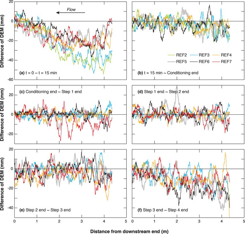
C. An et al.: Effect of stress history on sediment transport and channel adjustment                                              335

The threshold of motion is analyzed in Sect. 4 based on the
experimental data. Implications and limitations of this study
are also discussed in Sect. 4. Finally, conclusions are sum-
marized in Sect. 5.

2   Experimental arrangements

The experimental arrangements were guided by conditions
observed in East Creek, a small mountain creek in Malcolm
Knob Forest, University of British Columbia (for details on
the study site, see Papangelakis and Hassan, 2016). To inves-
tigate the study objectives, we conducted flume experiments
in the Mountain Channel Hydraulic Experimental Labora-
tory at the University of British Columbia. The experiments
were conducted in a tilting flume with a length of 5 m, a
width of 0.55 m, and a depth of 0.80 m. The initial slope was      Figure 1. Water and sediment supply implemented in the experi-
0.04 m/m. Water (but not sediment) was recirculated by an          ments. Markers at the top of the figure denote the time of measure-
axial pump. A set of six experiments (REF2–REF7) was con-          ments during the hydrograph phase. The time of the measurements
ducted; the experimental conditions are briefly summarized         during the conditioning phase is not shown in this figure.
in Table 1. For experiments REF3–REF7, the same hydro-
graph and sedimentograph were conducted but with differ-
ent durations of constant conditioning flow prior to the hy-       sedimentograph consisted of four steps, with each step last-
drograph or sedimentograph. It should be noted that in the         ing for 2 h.
experiments we only implemented the rising limb of the hy-            Figure 2 shows the GSD of the bulk sediment used in the
drograph or sedimentograph, rather than a full hydrograph or       experiments, with the grain size ranging between 0.5 and
sedimentograph with both rising and falling limbs. Rather          64 mm. The GSD was scaled from East Creek by a ratio of 1 :
than studying river adjustment during a flow hydrograph,           4, except that sediment (after scaling) with a grain size less
we aimed at determining the influence of conditioning time         than 0.5 mm was excluded. This preserved the entire gravel
on bed load and bed surface arrangements as flow rates in-         distribution of East Creek with a maximum size of 256 mm
creased. We denote these as REF3 (10), REF4 (2), REF5 (5),         (scaled to 64 mm in Fig. 2). The model was “generic” rather
REF6 (15), and REF7 (0.25), with the numbers in the brack-         than specific. This means that no attempt was made to re-
ets denoting the duration of the conditioning flow in hours.       produce the geometric details of the prototype channel. The
Experiment REF2 (15) consists of a 15 h conditioning pe-           bulk sediment was sieved at half ϕ intervals, and each grain
riod without a subsequent hydrograph or sedimentograph to          size class was painted in different colors for texture analysis
test the reproducibility of our experimental results during the    and visual identification. Before the commencement of each
conditioning flow.                                                 experiment, we hand-mixed and leveled the bulk sediment to
   Figure 1 shows the water and sediment supply imple-             make a flat and uniform layer of loose material with a depth
mented during the experiments. The water discharge was se-         of 0.15 m. The sediment was then slowly flooded and then
lected to represent typical flows in East Creek, with the 25 L/s   drained to aid settlement. The bulk sediment was also used
flow during the conditioning period being equivalent to half       for the sediment feed in each experiment.
the bankfull flow, and the peak flow discharge of 40 L/s dur-         The bed and water surface elevations were measured along
ing the hydrograph being about 1.1 times the bankfull flow         the flume every 0.25 m using a mechanical point gauge with a
in East Creek. Because the purpose of this paper is to study       precision of ±0.001 m. Water depth fluctuations due to wave
the evolution of bed stability, sediment was not fed during        effects at a point were about 5 % or less. Water surface slope
the conditioning flow. For each step of the hydrograph, the        and bed slope are calculated based on a linear regression of
feed rate of sediment was specified to be close to the trans-      the point gauge data measured between 0.5 and 4.75 m up-
port capacity of the flow. Determination of the sediment sup-      stream of the outlet. The most upstream and downstream sec-
ply rates was facilitated by a numerical model, which was          tions are excluded to avoid boundary effects. A green laser
calibrated for similar experimental conditions (Ferrer-Boix        scanner mounted on a motorized cart was also used to mea-
and Hassan, 2014). Sediment was fed into the flume at the          sure the bed surface elevation along the flume. Bed laser
upstream end using a conveyor belt feeder at the calculated        scans were composed of cross sections spaced 2 mm apart
transport rate capacity. The feed rate of the sedimentograph       with 1 mm vertical and horizontal accuracy (for details, see
ranged between 1 and 10 kg/h. Both the hydrograph and the          Elgueta-Astaburuaga and Hassan, 2017). The standard de-

https://doi.org/10.5194/esurf-9-333-2021                                                 Earth Surf. Dynam., 9, 333–350, 2021
C. An et al.: Effect of stress history on sediment transport and channel adjustment
https://doi.org/10.5194/esurf-9-333-2021
Table 1. Summary of the experimental conditions and measurements. The experiments are listed in the table in order of decreasing duration of conditioning flow.
No. Phase Duration Flow Water Flow Froude τb 1zb Sediment Ds50 Ds90 Dl50 Dl90 ∗
τs50 Qs
(h) discharge surface depth number (Pa) (mm) feed (mm) (mm) (mm) (mm) (kg/h)
(L/s) slope (%) (cm) (–) (kg/h)
REF2 (15) Conditioning 15 25 2.62 6.33 0.91 16.27 −30.2 0 15.5 29.7 1.07 5.43 0.065 0.27
REF6 (15) Conditioning 15 25 3.27 6.47 0.88 20.76 −16.6 0 15.7 30.8 35.18 42.84 0.082 0.89
Step 1 2 26 3.34 6.39 0.94 20.93 0.3 1 14.4 30.0 12.51 39.38 0.090 0.68
Step 2 2 28 3.10 6.29 1.03 19.13 0.0 1.5 17.3 29.4 7.28 27.59 0.068 0.76
Step 3 2 32 3.06 6.80 1.05 20.41 −1.9 3.2 16.2 31.8 12.39 36.54 0.078 6.73
Step 4 2 40 2.81 7.78 1.07 21.45 −16.1 10 15.9 31.6 11.48 36.03 0.083 13.39
REF3 (10) Conditioning 10 25 2.73 6.02 0.98 16.12 −25.8 0 14.8 29.2 2.17 9.98 0.067 0.28
Step 1 2 26 2.75 5.93 1.04 16.00 0.1 1 15.6 29.5 2.55 19.94 0.063 1.71
Step 2 2 28 2.69 6.35 1.01 16.77 0.3 1.5 15.8 30.2 4.06 26.99 0.065 2.19
Step 3 2 32 2.88 6.81 1.04 19.25 −1.7 3.2 15.9 30.1 6.18 24.26 0.075 2.44
Step 4 2 40 2.48 8.34 0.96 20.28 −8.0 10 14.2 32.8 14.45 39.13 0.088 12.45
REF5 (5) Conditioning 5 25 3.26 5.51 1.12 17.63 −16.8 0 15.3 32.0 8.23 25.34 0.071 0.49
Step 1 2 26 3.24 6.19 0.98 19.68 −0.6 1 15.4 31.5 6.57 23.63 0.079 2.24
Step 2 2 28 3.09 6.21 1.05 18.82 −0.3 1.5 17.2 31.4 9.38 28.44 0.067 3.30
Step 3 2 32 3.05 6.65 1.08 19.91 −1.2 3.2 16.8 31.9 11.90 47.91 0.073 5.72
Step 4 2 40 2.78 7.82 1.06 21.33 −13.4 10 15.1 34.5 15.09 38.56 0.087 40.03
REF4 (2) Conditioning 2 25 2.82 5.55 1.11 15.34 −17.8 0 12.3 27.8 3.10 15.79 0.077 1.50
Step 1 2 26 2.73 5.55 1.16 14.85 −0.5 1 14.8 28.9 3.90 20.31 0.062 0.96
Step 2 2 28 2.71 6.19 1.06 16.46 −0.1 1.5 15.6 29.2 6.28 46.76 0.065 2.41
Step 3 2 32 3.15 6.85 1.04 21.15 −6.4 3.2 14.5 28.8 17.34 37.76 0.090 26.73
Earth Surf. Dynam., 9, 333–350, 2021
Step 4 2 40 2.76 8.01 1.02 21.69 −7.7 10 13.7 29.7 10.88 35.45 0.098 5.23
REF7 (0.25) Conditioning 0.25 25 3.46 6.20 0.94 21.06 −14.9 0 14.0 29.5 10.54 28.03 0.093 19.44
Step 1 2 26 3.20 6.54 0.90 20.53 −4.8 1 15.6 31.6 7.11 28.91 0.081 3.48
Step 2 2 28 3.14 6.58 0.96 20.27 −0.7 1.5 16.2 21.2 6.91 30.73 0.077 2.52
Step 3 2 32 3.12 7.00 1.00 21.41 −4.5 3.2 14.3 30.5 10.09 37.40 0.092 12.32
Step 4 2 40 2.73 8.29 0.97 22.19 −9.6 10 17.3 33.6 12.13 30.78 0.079 16.80
Qs : bed load transport rate; 1zb : mean difference of bed elevation averaged over the whole river channel; τb : shear stress; Ds50 and Ds90 : D50 and D90 of bed surface; Dl50 and Dl90 : D50 and D90 of bed load; τs50 ∗ : Shields
number for Ds50 . Here D90 denotes the grain size such that 90 % is finer, and D50 denotes the grain size such that 50 % is finer. All values presented in this table are measured at the end of each stage, except for 1zb , which
denotes the mean difference of bed elevation during each stage (i.e., difference between the end of this stage and the end of last stage). A positive value of 1zb denotes aggradation, and a negative value of 1zb denotes
degradation.
336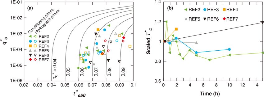
C. An et al.: Effect of stress history on sediment transport and channel adjustment                                              337

                                                                     parameters controlling bed evolution; in addition, the water
                                                                     was too shallow to use an ADV. The water surface slope,
                                                                     rather than bed slope, is implemented in the calculation of
                                                                     shear stress, with the consideration that water surface slope
                                                                     is closer to the friction slope and also has less random fluctu-
                                                                     ations than bed slope.
                                                                        The frequency of measurements during the hydrograph
                                                                     phase is also plotted in Fig. 1a, with the point gauge mea-
                                                                     surements conducted every 30 min, the trap weighting and
                                                                     sampling conducted every hour, and the DEM and Wolman
                                                                     measurements by laser scan and photograph conducted ev-
                                                                     ery 2 h (i.e., at the beginning and end of each stage of the
                                                                     hydrograph). For each measurement of DEM and Wolman,
                                                                     we stopped the pump instantaneously and let the flow slowly
                                                                     lower and then stop to allow for the bed to be scanned by a
                                                                     laser and photographed. The time interval between the stop
Figure 2. Grain size distribution of the bulk sediment used in the   of the pump and the stop of the flow was about 3 to 4 min. To
experiments.
                                                                     avoid the influence of the following rising discharge, all sub-
                                                                     sequent measurements were taken after the flow became sta-
                                                                     ble. The frequency of measurement during the conditioning
viation of bed elevation was calculated based on the digital         phase was adjusted in each experiment in accordance with
elevation model (DEM) data from scans. Before the calcula-           the duration of the conditioning phase and is therefore not
tion of standard deviation, the DEM was detrended based on           plotted in Fig. 1.
linear regression to remove spatial trends with scales larger           The uncertainties associated with the measurement are
than the scale of sediment patterns (e.g., bed slope or undu-        also studied. For the uncertainties of the standard deviation
lations). To estimate the particle size distribution of the bed      of bed elevation, we scanned the floor of the flume twice and
surface we used digital cameras mounted on a motorized cart          calculated the standard deviations of the scanned DEM. The
along the entire flume. Images were merged together to vi-           floor of the flume was horizontal and flat, with no sediment
sualize the bed and perform the particle size analysis (Char-        on the bed. Theoretically, the standard deviation of the DEM
trand et al., 2018). To avoid distortion effects due to image        should be zero. Therefore, the calculated standard deviations
merging, the width of the image strips that were stitched to         of the flume floor are regarded as an estimation of the un-
get a composite image was specified as just 2 cm. The parti-         certainties of our calculations during the experiment. To esti-
cle size distribution of the bed surface was estimated using         mate the uncertainties of the bed surface GSD, for each mea-
the Wolman (point count) method by identifying the grain             surement the Wolman method was implemented five times on
size of particles at the intersections of a 5 cm grid superim-       the same photograph, with 100 samples or counts each time.
posed on the photograph. Individual grains were identified           The five measured GSDs for each time interval were used to
by color. For each experiment, the grain size distribution of        calculate the mean and standard deviation of the bed surface
the bed surface was calculated at different times to quantify        texture (in terms of Ds10 , Ds50 , and Ds90 ). To estimate the
its changes during the experiment.                                   uncertainties of the light table method, we compare the data
   The sediment transport rates for various size ranges were         measured by the light table with the data measured by the
measured at the end of the flume using a light table (for de-        sediment trap, in terms of both sediment transport rate and
tails, see Zimmerman et al., 2008; Elgueta-Astaburuaga and           the characteristic grain sizes of sediment load. To estimate
Hassan, 2017) and automated image analysis at a resolution           the variations of the measured and calculated data, we calcu-
of 1 s. Material evacuated from the flume was trapped in a           late their coefficient of variation (cv), defined as the ratio of
0.25 mm mesh screen in the tailbox, weighted and sieved              the standard deviation to the mean value.
at half ϕ intervals, and then used to calibrate the light ta-
ble data. To avoid random fluctuations in sediment transport,
we report the bed load transport rate measured by light ta-          3   Experimental results
ble at a 5 min resolution and characteristic grain sizes of bed
load at 15 min resolution. A range of methods for the estima-        Table 1 presents an overall schematization of the experi-
tion of bed shear stress has been suggested in the literature        mental results, including water surface slope, flow depth
(reviewed in Whiting and Dietrich, 1990). In this study, the         h, Froude number F r (F r = u/(gh)0.5 ), where u is depth-
shear stress is estimated using the depth–slope product corre-       averaged flow velocity), bed load transport rate Qs , shear
sponding to normal (steady and uniform) flow. This method            stress τb , D50 and D90 of bed surface (Ds50 and Ds90 ), D50
is selected because the focus of this work is on overall (mean)      and D90 of bed load (Dl50 and Dl90 ), and Shields number

https://doi.org/10.5194/esurf-9-333-2021                                                  Earth Surf. Dynam., 9, 333–350, 2021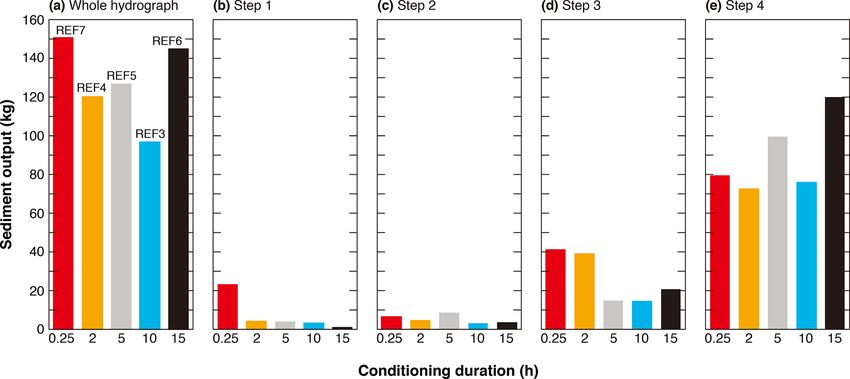
338 C. An et al.: Effect of stress history on sediment transport and channel adjustment
∗ for a given D . D
τs50 s50 90 denotes the grain size such that conditioning phase, as well as during the hydrograph phase,
90 % is finer, and D50 denotes the grain size such that 50 % despite the fact that degradation is evident as the flow ap-
is finer. proaches its peak value. For the standard deviation of bed el-
evation during the conditioning phase, we calculate the coef-
3.1 Channel adjustment
ficient of variation (cv) for REF2 (15), which has the longest
conditioning phase. The result shows a value of 0.038 from
In this section, we present the channel adjustments during t = 15 min to the end of the conditioning flow. For the stan-
each experiment. Figure 3 shows the difference of longitu- dard deviation of bed elevation during the hydrograph phase,
dinal DEM averaged over the cross section, which can rep- we calculate the cv for all experiments; the results show that
resent the adjustment of channel topography during differ- the values of cv vary between 0.031 and 0.075. Besides, the
ent periods of the experiment. The DEM averaged over the value of standard deviation is almost identical for each ex-
cross section is used here to study the overall aggradation or periment, indicating the period of conditioning phase exerts
degradation of the channel. For reference, detailed informa- little effect on the standard deviation of bed elevation.
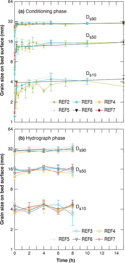
tion about the DEM at different times during the experiment Figure 5 shows the temporal variation of the characteris-
is provided in the Supplement, with REF6 (15) as an exam- tic grain size of bed surface material, as well as an estima-
ple. From Fig. 3a we can see that, for each experiment, ev- tion of the uncertainties associated with measurements of the
ident degradation occurs during the first 15 min, especially surface texture. Three parameters are presented here: Ds10 ,
at the upstream end of the flume. This is due to the fact that Ds50 , and Ds90 . The adjustment of bed surface GSD follows
no sediment supply is implemented during the conditioning similar trends to the adjustment of standard deviation of bed
period and the initial bed material is relatively loose. From elevation; i.e., for all experiments the bed surface is fine at
15 min until the end of the conditioning phase (as shown in the beginning and experiences a fast coarsening period dur-
Fig. 3b), no evident aggradation or degradation is observed ing the first 15 min (along with the bed degradation in Fig. 3
for any experiment, indicating that most of the adjustment of and the increase of bed roughness in Fig. 4). The character-
channel topography during the conditioning phase has been istic grain sizes of bed surface remain relatively stable after
accomplished within the first 15 min. For step 1 of the hydro- the first 15 min, despite variabilities due to the measurement
graph (as shown in Fig. 3c), no evident aggradation or degra- uncertainty. For REF2 (15), which has the longest condition-
dation is observed for any of the experiments (with the mean ing phase, cv (coefficient of variation) values of the mean
difference of bed elevation 1zb less than ±1 mm, as shown Ds10 , Ds50 , and Ds90 (over the five repeated measurements)
in Table 1), except for REF7 (0.25), which has the shortest are 0.15, 0.09, and 0.02, respectively, from t = 15 min to the
conditioning phase and experienced a mean degradation of end of the conditioning flow. It is worth noting that the GSD
4.8 mm over the whole bed channel. Similarly, the channel of bed surface remains relatively constant even during the hy-
remains relatively stable during step 2 of the hydrograph for drograph phase, during which a flood event is introduced in
all experiments (as shown in Fig. 3d), with no evident aggra- the flume and evident bed degradation is observed. For each
dation or degradation being observed (the mean difference of experiment, the cv values of the mean Ds10 , Ds50 , and Ds90
bed elevation 1zb is less than ±1 mm for all experiments). (over the five repeated measurements) are less than 0.13,
With the increase of flow discharge, some degradation (with 0.08, and 0.04, respectively, during the hydrograph phase.
a magnitude of about 10–20 mm) can be observed in step 3
for all experiments at the upstream end of the channel, as 3.2 Sediment transport
shown in Fig. 3e. Such degradation becomes more evident
over the entire channel in step 4 of the hydrograph, when In Fig. 6 we present the instantaneous sediment transport
flow discharge reaches its peak value. This is in agreement rate Qs measured by the light table during each experiment.
with the values of 1zb presented in Table 1. Sediment transport is reported every 5 min, as described in
Figure 4 shows the temporal variation of the standard de- Sect. 2. Accuracy of the results is estimated by comparing
viation of bed elevation, which is often scaled with the bed the light table data with the data measured by the trap. Re-
roughness for gravel-bed rivers (see Chen et al. 2020, for a sults show that for our experiments, the light table method
detailed discussion on this topic), over the length of the erodi- has good accuracy in terms of the sediment transport rate,
ble bed during the experiment. Results show that the standard with an overestimation by 4 % on average (111 samples and
deviation of bed elevation is relatively small at the beginning a standard deviation of 14.5 %). A total of 70 out of 111 sam-
of the experiments (corresponding to a relatively smooth bed ples show an accuracy of ±10 %, and 93 out of 111 samples
depending on the way we prepared the initial bed) but in- show an accuracy of ±20 %. Details of this uncertainty anal-
creases notably within 15 min after the start of the condition- ysis are presented in the Supplement.
ing phase. Such an increase of the standard deviation of bed It can be seen in Fig. 6a that the temporal variation of sed-
elevation is accompanied by significant degradation during iment transport rate during the conditioning phase follows
the first 15 min, as shown in Fig. 3a. The standard deviation the same trend in all six experiments. That is, the sediment
of bed elevation becomes quite stable during the remaining transport rate decreases significantly during the conditioning
Earth Surf. Dynam., 9, 333–350, 2021 https://doi.org/10.5194/esurf-9-333-2021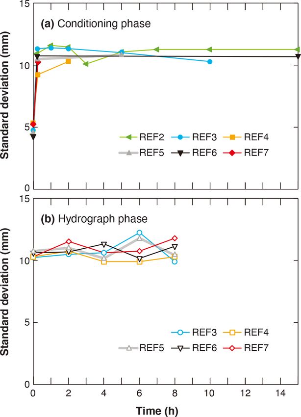
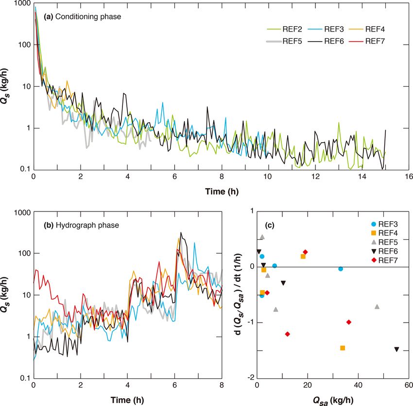
C. An et al.: Effect of stress history on sediment transport and channel adjustment                                                     339

Figure 3. Spatial distribution of elevation difference from cross-sectionally averaged longitudinal DEM during the experiment: (a) from the
beginning of the experiment to t = 15 min, (b) from t = 15 min to the end of the conditioning phase, (c) from the end of the conditioning
phase to the end of step 1 of the hydrograph phase, (d) from the end of step 1 to the end of step 2 of the hydrograph phase, (e) from the end
of step 2 to the end of step 3 of the hydrograph phase, and (f) from the end of step 3 to the end of step 4 of the hydrograph phase.

phase, with the decreasing rate being very large at the be-              spikes imply that partial destruction (or reorganization) of the
ginning and then gradually dropping. In the first 15 min, the            bed structure occurs even after a long duration of condition-
sediment transport rates drop from more than 500 kg/h to less            ing.
than 100 kg/h. Afterwards, it takes about another 2 h for the               Previous researchers (Haynes and Pender, 2007; Masteller
sediment transport rates to drop to close to 1 kg/h. The sed-            and Finnegan, 2017) have suggested that an exponential
iment transport rate eventually approaches a small and rela-             function can be implemented to describe such a decrease of
tively constant value after about 8 h of conditioning flow. For          sediment transport rate under conditioning flow. Additional
REF2 (15) and REF6 (15), which have the longest condition-               analysis is implemented in the Supplement to fit REF2 (15)
ing phase, the sediment transport rates between t = 8 h and              and REF6 (15) (which have the longest duration of condi-
the end of conditioning phase (t = 15 h) show mean values                tioning phase) against a two-parameter exponential function.
of 0.35 kg/h (standard deviation = 0.22 kg/h) and 0.37 kg/h              Results show that the exponential function can describe the
(standard deviation = 0.24 kg/h), respectively. Nevertheless,            general decreasing trend of sediment transport rate during the
there are random high points in the sediment transport rate              conditioning phase, except at the beginning of the experiment
even after 8 h, despite no sediment feed from the inlet. These           where the decrease of sediment transport rate is much more

https://doi.org/10.5194/esurf-9-333-2021                                                        Earth Surf. Dynam., 9, 333–350, 2021
340                                         C. An et al.: Effect of stress history on sediment transport and channel adjustment

Figure 4. Temporal adjustments of standard deviation of bed ele-
vation calculated over the whole erodible bed: (a) the conditioning
phase and (b) the hydrograph phase. The uncertainty of the calcu-
lation is in the range of 1.6–2.5 mm, which is close to the vertical
resolution of the laser (1 mm).

significant than that predicted by the exponential function.
Readers can refer to the Supplement for more details.
   Figure 6b presents the instantaneous sediment transport
rate during the hydrograph phase. Results show that varia-             Figure 5. Temporal adjustments of characteristic grain sizes of bed
tion of sediment transport rate among different experiments            surface material calculated over the whole erodible bed: (a) the con-
prevails in the first step of the hydrograph, with the highest         ditioning phase and (b) the hydrograph phase. Markers show mean
sediment transport rate for the experiment with the shortest           values of five repeated Wolman measurements. Range bars show the
                                                                       mean values ± the standard deviations of the five repeated Wolman
conditioning duration (REF7 (0.25)) and the smallest sedi-
                                                                       measurements.
ment transport rate for the experiment with the longest con-
ditioning duration (REF6 (15)). Such variation among exper-
iments, however, diminishes towards the end of step 1 and
is not observed in the following three steps of the hydro-             step variations of sediment transport rate are investigated in
graph, with the line for each experiment collapsing together           Fig. 6c, with the x axis being the averaged sediment transport
in the figure. Such adjustments of sediment transport rate are         rate of each step Qsa and the y axis being d(Qs /Qsa )/dt. The
consistent with the process of channel deformation shown               value of d(Qs /Qsa )/dt is estimated by linear regression. Here
in Fig. 3. Thus, for both sediment transport and channel de-           the instantaneous sediment transport rate Qs is scaled against
formation, results of REF7 (0.25) deviate from other exper-            the average sediment transport rate of the corresponding step
iments in step 1 (larger sediment transport rate and more              Qsa in order to facilitate the comparison among different hy-
degradation in REF7 (0.25)) but collapse with other exper-             drograph steps.
iments in the following three steps.                                      Results in Fig. 6c show that a large fraction of the data
   Results in Fig. 6b also show large variations of sediment           (11 out of 20) exhibit a decreasing trend in time for Qs
transport rate during each step of the hydrograph. Such intra-         (i.e., a negative value in vertical coordinate). Basically, the

Earth Surf. Dynam., 9, 333–350, 2021                                                       https://doi.org/10.5194/esurf-9-333-2021
C. An et al.: Effect of stress history on sediment transport and channel adjustment 341 Figure 6. Instantaneous sediment transport rate measured by the light table during (a) the conditioning phase and (b) the hydrograph phase. (c) Intra-step temporal change rate of Qs normalized against Qsa for each hydrograph step. Qs is the sediment transport rate, and Qsa is the averaged sediment transport rate of a given hydrograph step. larger the averaged sediment transport rate Qsa , the larger evidently higher. The decreasing and increasing trends of Qs the rate of reduction in Qs . Ferrer-Boix and Hassan (2015) during steps of the hydrograph reflect the transient adjust- observed similar declines in sediment transport during their ments of the bed to the changed water and sediment supply water pulse experiments. They attributed this to (1) the pres- before equilibrium is achieved. ence of bed structures, which could have reduced skin fric- Sediment collected in the trap or tailbox at the flume outlet tion up to 20 %, and (2) streamwise changes in the patterns of allows us to plot the total amount of sediment output dur- bed surface sorting. Out of 20 datasets, 5 exhibit some tem- ing each step of the hydrograph. Figure 7a shows the to- porally increasing trend in Qs (though this is not as evident as tal sediment output during the entire hydrograph. It can be the decreasing trend mentioned before). They are REF5 (5), seen that the effect of conditioning duration on the total sed- REF3 (10), REF6 (15) during the first step and REF7 (0.25), iment output during the entire hydrograph phase is not ev- REF4 (2) during the third step. This shows that for the three ident: a longer duration of conditioning flow does not nec- experiments with a long conditioning duration, Qs is very essarily lead to a smaller (or larger) sediment output. The low at the end of the conditioning phase, and the first step largest sediment output occurs in REF7 (0.25), which is 55 % of the hydrograph sees a temporally increasing trend in Qs , larger than the sediment output in REF3 (10), which has the whereas for the two experiments with a short conditioning smallest output, but is about the same as (only 4 % larger phase, Qs is still high at the end of the conditioning, and thus than) the sediment output in REF6 (15). We further calculate the sediment transport rate keeps decreasing during the first the correlation coefficient between the total sediment output step until an increasing trend in Qs is observed in the third and the duration of conditioning flow and obtain a value of step, at which point the water and sediment supply become https://doi.org/10.5194/esurf-9-333-2021 Earth Surf. Dynam., 9, 333–350, 2021
342                                         C. An et al.: Effect of stress history on sediment transport and channel adjustment

r = −0.14, indicating that there is almost no correlation be-         39.0 %) for Dl10 and an overestimation by 30 % on average
tween the two parameters.                                             (111 samples and a standard deviation of 26.5 %) for Dl90 .
   However, if we study the sediment transport during each            Details concerning this uncertainty analysis are presented in
step of the hydrograph, we can find that in step 1 REF7               the Supplement.
(0.25) has much larger sediment output than the other ex-                The value of Dl10 shows a decreasing trend during the con-
periments, as shown in Fig. 7b. For Step 1, the sediment              ditioning phase (Fig. 8a), with a value of more than 2 mm at
output is 1.1 in REF6 (15); 3.4–4.4 kg in REF4 (2), REF5              the beginning to about 0.6 mm after 15 h, in spite of the large
(5), and REF 3(10); and increases sharply to 23.4 kg in REF7          fluctuations before 8 h. The decrease of Dl10 reflects an in-
(0.25) (which is more than 20 times that in REF6 (15)). This          crease in the fraction of the finest sediment in bed load. In
agrees with the results for instantaneous sediment transport          the first two steps of the hydrograph (Fig. 8b), the value of
rate shown in Fig. 6b and shows that the duration of condi-           Dl10 is relatively stable for experiments with long condition-
tioning flow can influence the sediment transport at the be-          ing phases (i.e., REF6 (15) and REF3 (10)) but shows a de-
ginning of the subsequent flood, with a longer conditioning           creasing trend along with fluctuations for experiments with
phase leading to less sediment transport. When the duration           short conditioning phases (i.e., REF7 (0.25), REF4 (2), and
of conditioning flow is over 2 h, the subsequent sediment             REF5 (5)). The last two steps of the hydrograph see an ev-
transport rate becomes rather insensitive to further increase         ident increase in the value of Dl10 compared with the first
of conditioning duration, indicating that the reorganization          two steps, due to the increase of flow discharge and sediment
of the river bed under conditioning flow is mostly finished           supply (Fig. 8b). We note that such an increase in the Dl10 is
within 2 h. The effects of stress history on subsequent sedi-         larger than the standard deviation of measurements, as shown
ment transport can hardly be observed during step 2 of the            above.
hydrograph (Fig. 7c). Sediment output in REF7 (0.25) re-                 Figure 8c and d show the temporal variation of Dl50 . Com-
duces significantly to a similar magnitude to the other exper-        pared with that of Dl10 , the temporal variation of Dl50 shows
iments because most of the loose bed material in REF7 (0.25)          more significant fluctuations during the conditioning phase
has been moved by the end of step 1. More specifically, the           (especially after t = 10 h), as well as at the beginning of the
volumes of sediment output in this step range between 3.1             hydrograph. This can be shown by the coefficient of varia-
and 8.6 kg, with the largest output occurring in REF5 (5)             tion (cv) of the grain size. For the conditioning phase (af-
and the minimum output occurring in REF3 (10). We further             ter t = 10 h), the cv of Dl10 shows an average value of 0.05,
calculate the correlation coefficient between sediment output         whereas the cv of Dl50 shows an average value of 1.44. For
and conditioning duration and obtain a value of r = −0.61,            step 1 of the hydrograph phase, the cv of Dl10 shows an av-
indicating that a longer conditioning duration can no longer          erage value of 0.35, whereas the cv of Dl50 shows an aver-
lead to a larger sediment output in this step. In Step 3 of the       age value of 0.66. For step 2 of the hydrograph phase, the
hydrograph (Fig. 7d), sediment output in REF7 (0.25) and              cv of Dl10 shows an average value of 0.12, whereas the cv
REF4 (2) is larger than in other three experiments, which             of Dl50 shows an average value of 0.54. As for the temporal
have longer conditioning phases. However, in this step the            variation of Dl90 (in Fig. 8e and f), the fluctuations are still
sediment output in REF7 (0.25) is no more than 3 times that           significant, with the average cv being 0.61, 0.34, and 0.27
of the sediment output in REF3 (10), which has the minimum            for the conditioning phase (after t = 10 h), step 1 of hydro-
sediment output. This difference of sediment output among             graph phase, and step 2 of hydrograph phase, respectively.
experiments is not as significant as in step 1. In the last step of   Besides, there is no significant increase or decrease of Dl90
the hydrograph, with the flow discharge and sediment supply           during the experiment. This indicates that the transport of the
approaching their peaks, the difference in sediment output            coarsest sediment is not sensitive to the variation of our ex-
among the five experiments again becomes small, with the              perimental conditions. The more significant fluctuations in
values ranging between 72.1 kg in REF4 (2) and 119.6 kg in            Dl50 and Dl90 might be attributed to the fact that during rela-
REF6 (15). This demonstrates that little influence of stress          tively low flow coarse sediment is more likely to be near the
history remains in this step.                                         threshold of motion and move intermittently, e.g., as individ-
   Figure 8 shows the temporal variation of the grain size dis-       ual grains, as opposed to the more continuous movement for
tribution of the bed load. Here Dl10 , Dl50 , and Dl90 denote         fine sediment. These fluctuations gradually diminish with the
grain sizes such that 10 %, 50 %, and 90 % are finer in the           increase of flow and sediment supply, as the static armor on
bed load, respectively. Accuracy of the measurements is es-           bed surface transits to mobile armor and the movement of
timated by comparing the light table data with the trap data.         coarse grains becomes more continuous.
Results show that for our experiments, the light table method            With the fractional sediment transport rate measured by
has good accuracy in terms of the median size of bed load             the light table, we also analyze the sediment mobility of each
(Dl50 ), with an overestimation by 3 % on average (111 sam-           size range during the experiment. Results show that sedi-
ples and a standard deviation of 40.1 %). Measurements of             ment transport rate is characterized by equal mobility (i.e.,
Dl10 and Dl90 show less accuracy, with an underestimation             the GSD of sediment load matches the GSD of sediment on
by 20 % on average (111 samples and a standard deviation of           bed surface) at the beginning of the conditioning phase but

Earth Surf. Dynam., 9, 333–350, 2021                                                     https://doi.org/10.5194/esurf-9-333-2021
C. An et al.: Effect of stress history on sediment transport and channel adjustment                                                 343

Figure 7. Sediment output measured at a trap during (a) the whole hydrograph, (b) step 1 of the hydrograph, (c) step 2 of the hydrograph,
(d) step 3 of the hydrograph, and (e) step 4 of the hydrograph.

Figure 8. Temporal adjustments of characteristic grain sizes of bed load: (a) Dl10 during conditioning phase, (b) Dl10 during hydrograph
phase, (c)Dl50 during conditioning phase, (d) Dl50 during hydrograph phase, (e) Dl90 during conditioning phase, and (f) Dl90 during
hydrograph phase.

https://doi.org/10.5194/esurf-9-333-2021                                                     Earth Surf. Dynam., 9, 333–350, 2021
344                                      C. An et al.: Effect of stress history on sediment transport and channel adjustment

moves to partial or selective mobility after a relatively long    mations with the three different methods show a very similar
conditioning phase and during the first two steps of the hy-      temporal trend and variability.
drograph. However, with the increase of flow discharge and                                                    ∗ for each exper-
                                                                     Figure 9a shows the values of qs∗ vs. τs50
sediment supply, the sediment transport regime gradually re-      iment, along with the Wong and Parker (2006) type relation
turns to equal mobility during the last two steps of the hy-      (Eq. 1) with various values for τc∗ (from 0.04 to 0.09). It can
drograph. Details of the analysis are presented in the Supple-    be seen from the figure that the measured sediment trans-
ment.                                                             port rate is relatively low, with most points below the di-
                                                                  mensionless value of 0.001. This indicates that the Shields
                                                                  number in our experiment is slightly larger than the critical
4     Discussion                                                  Shields number, a state that is typical for gravel-bed rivers
                                                                  (Parker, 1978). The four points with dimensionless transport
4.1    Threshold of sediment motion in experiments                rate above 0.001 are all at the beginning of the condition-
The threshold of sediment motion is a key parameter for           ing flow (t = 15 min). The values of qs∗ basically show an
                                                                  increasing trend with the increase of τs50∗ , with the correla-
the prediction of bed load transport. Previous studies on the                                ∗            ∗
stress history effect often start with a conditioning flow that   tion coefficient between τs50 and log(qs ) (consistent with the
is below the threshold of motion and then gradually increase      semi-log scale of Fig. 9a) being 0.58. Besides, the values of
the flow discharge so that the threshold of motion can be di-     critical Shields number τc∗ shown in Fig. 9a cover a rather
rectly estimated in the experiment (e.g., Monteith and Pen-       wide range (from less than 0.06 to larger than 0.09).
der, 2005; Masteller and Finnegan, 2017; Ockelford et al.,           Table 2 shows the values of τc∗ back-calculated at the be-
2019; etc.). Because our experiments implement a condition-       ginning (t = 15 min) and the end of the conditioning phase
ing flow which can mobilize sediment (sediment transport at       in each experiment. The back-calculated values of τc∗ vary in
the beginning of the conditioning phase is especially large),     the range 0.065–0.090 for the conditioning phase, which is
the threshold of motion cannot be observed directly in the        well above the value of 0.0495 recommended by Wong and
experiment. Here we follow the method applied in Hassan           Parker (2006). Lamb et al. (2008) demonstrated that critical
et al. (2020) and estimate the threshold of sediment motion       shear stress can become larger for large bed slope, and they
with the Wong and Parker (2006) sediment transport relation,      proposed a relation which considers the effect of bed slope,
which is a revision of the Meyer-Peter and Müller (1948) re-      τc∗ = 0.15Sb0.25 ,                                           (5)
lation.
   We use the Wong and Parker (2006) relation, which main-        where Sb is bed slope. For comparison, Table 2 also shows
tains the exponent 1.5 of Meyer-Peter and Muller (1948):          the values of τc∗ calculated by Eq. (5). Results shows that
                                                                  for the conditioning phase of our experiments, τc∗ calculated
                     1.5                                         by Eq. (5) is above 0.06, which is much higher than the rec-
qs∗ = 3.97 τs50
             ∗
                − τc∗ ,                                    (1)
                                                                  ommended value of Wong and Parker (2006). Besides, the τc∗
            qs
qs∗ = √               ,                                    (2)    values predicted by the Lamb et al. (2008) relation show little
         RgDs50 Ds50                                              variability among different experiments, compared with the
  ∗        τb                                                     values back-calculated with Eq. (1) based on experimental
τs50 =           ,                                         (3)
        ρgRDs50                                                   data. More specifically, the cv values are 0.032 at t = 15 min
τb = ρghSw ,                                               (4)    and 0.031 at the end of the conditioning phase for τc∗ pre-
                                                                  dicted by Lamb et al. (2008) relation but become 0.10 at
where qs∗ is the dimensionless bed load transport rate (Ein-      t = 15 min and 0.12 at the end of the conditioning phase
stein number) defined by Eq. (2), τs50∗ is the Shields num-       for τc∗ back-calculated with Eq. (1) using measured data.
ber for surface median grain size Ds50 defined by Eq. (3),        Such discrepancies could be ascribed to the fact the relation
τb is the flow shear stress calculated using the depth–slope      of Lamb et al. (2008) considers only the influence of bed
product (Eq. 4), τc∗ is the critical Shields number for the       slope, without considering the effects of other mechanisms
threshold of sediment motion, qs is the volumetric sediment       like organization of surface texture, infiltration of fine parti-
transport rate per unit width, h is water depth, Sw is wa-        cles, etc. These potential effects are discussed in more detail
ter surface slope, R = 1.65 is the submerged specific grav-       in Sect. 4.2.
ity of sediment, g = 9.81 m/s2 is the gravitational acceler-         Here we also estimate the uncertainties associated with the
ation, and ρ = 1000 kg/m3 is the water density. Wong and          calculation of τc∗ . For τc∗ back-calculated with Eq. (1), the
Parker (2006) proposed a value of 0.0495 for τc∗ in Eq. (1).      global uncertainty is estimated by combining the uncertain-
                         ∗ from the measured data of the ex-
Here we obtain qs∗ and τs50                                       ties of each parameter involved in the calculation, i.e., water
periments and back-calculate the value of τc∗ using Eq. (1). It   depth h, water surface slope Sw , sediment transport rate qs ,
is worth mentioning that in Hassan et al. (2020) three differ-    and surface median grain size Ds50 . The applied ranges of h
ent methods, including the method as described above, are         and Sw are the measured values plus or minus the errors as-
applied to estimate the threshold of sediment motion. Esti-       sociated with the gauge point. The applied ranges of qs and

Earth Surf. Dynam., 9, 333–350, 2021                                                   https://doi.org/10.5194/esurf-9-333-2021
C. An et al.: Effect of stress history on sediment transport and channel adjustment 345
∗ using surface median grain size for measured transport rates
Figure 9. (a) Dimensionless sediment transport rate qs∗ vs. Shields number τs50
(points). Also shown are lines for the Wong and Parker (2006) type equation (Eq. 1) using different values for τc∗ . (b) Temporal adjustment of
scaled τc∗ (τc∗ over τc∗ at 15 min) during the conditioning phase. Here τc∗ is back-calculated using Eq. (1) (Wong and Parker, 2006, relation).
Ds50 are the measured values plus or minus the standard de- 4.2 Implications and limitations
viations as reported in Sect. 3. Results of the uncertainties
are presented in the brackets in Table 2. For the τc∗ values Previous research has shown that antecedent conditioning
calculated with Eq. (5), the uncertainties are only from the flow can lead to an increased critical shear stress and re-
bed slope Sw (which is related with the resolution of point duced sediment transport rate during subsequent flood event
gauge) and are lower than ±1 % according to our estimates. (Hassan and Church, 2000; Haynes and Pender, 2007; Ock-
Therefore, the uncertainty of τc∗ calculated with the Eq. (5) elford and Haynes, 2013; Masteller and Finnegan, 2017).
is not presented in the table. It can be seen from Table 2 that Our flume experiments also show a reduction in sediment
the values of τc∗ calculated with the Eq. (5) are mostly within transport rate, especially at the beginning of the hydrograph,
the uncertainty range of τc∗ back-calculated with Eq. (1), with in response to the implementation of antecedent condition-
the values closer to the lower bound of the uncertainty range. ing flow (as shown in Figs. 6b and 7). However, our results
In Fig. 9b, we plot the scaled τc∗ during the conditioning are different from previous research in that the influence of
phase of our experiments. For each experiment, the scaled antecedent conditioning flow is found to last for a relatively
τc∗ is calculated as the ratio between τc∗ and the correspond- short time at the beginning of the following hydrograph and
ing τc∗ at t = 15 min. τc∗ implemented here is back-calculated then gradually diminish with the increase of flow intensity
with Eq. (1). The scaled τc∗ collapses on a value of unity at and sediment supply (Figs. 6 and 7). Such results indicate
t = 15 min (i.e., the first point of each experiment). It can that increasing flow intensity and sediment supply during a
be seen from Fig. 9 that different trends are exhibited for flood event can lead to the loss of memory of stress history. A
the adjustment of τc∗ from t = 15 min to the end of condi- similar phenomenon was observed by Mao (2018) in his ex-
tioning phase, with REF2 (15) and REF3 (10) exhibiting a periment, where sediment transport during a high-magnitude
decreasing trend, REF5 (5) exhibiting very slight changes, flood event was not affected much by the occurrence of
and REF4 (2) and REF6 (15) exhibiting an increasing trend. lower-magnitude flood event before. Besides, the subsequent
The decrease of τc∗ in REF2 (15) and REF3 (10) is accom- hydrograph leads to evident bed degradation (Fig. 3) and in-
panied by a reduction of Shields number τs50 ∗ , mainly due
crease of sediment transport rate (Figs. 6 and 7) but does not
to the increase of surface median grain size Ds50 . Moreover, lead to evident change of surface texture or break of the ar-
the variation of back-calculated τc∗ is mostly within a range mor layer (Fig. 5). This is in agreement with the observation
of ±20 %, in agreement with our observation that variation of Ferrer-Boix and Hassan (2015) during experiments of suc-
of bed topography and bed surface texture become insignifi- cessive water pulses.
cant after 15 min. It should be noted that τc∗ cannot be back- Our results have practical implications for mountain
calculated using Eq. (1) within the first 15 min of the con- gravel-bed rivers. The importance of conditioning flow has
ditioning phase, since the information for flow depth, water long been discussed in the literature, and researchers have
surface slope, and bed surface GSD is not available. Nev- suggested that the stress history effect be considered in the
ertheless, we expect the adjustment of τc∗ could be evident modeling and analysis of gravel-bed rivers. For example, pre-
within the first 15 min, since the adjustments of both bed to- vious research states that existing sediment transport theory
pography and bed surface are significant during this period for gravel-bed rivers (e.g., Meyer-Peter and Müller, 1948;
(as shown in Sect. 3.1). Wilcock and Crowe, 2003; Wong and Parker, 2006; etc.)
might lead to unrealistic predictions if the stress history ef-
https://doi.org/10.5194/esurf-9-333-2021 Earth Surf. Dynam., 9, 333–350, 2021346 C. An et al.: Effect of stress history on sediment transport and channel adjustment
Table 2. Values of τc∗ at the beginning (t = 15 min) and the end of conditioning phase in each experiment. Here τc∗ is back-calculated with
Eq. (1). Also shown here are values of τc∗ estimated with the equation of Lamb et al. (2008) for comparison. Values in the brackets denote
the range of uncertainty associated with the τc∗ values back-calculated with Eq. (1).
t = 15 min End of conditioning
Back-calculated Lamb et al. Back-calculated Lamb et al.
by Eq. (1) (2008) by Eq. (1) (2008)
REF2 (15) 0.073 (0.064, 0.083) 0.063 0.065 (0.057, 0.074) 0.061
REF6 (15) 0.068 (0.053, 0.089) 0.066 0.081 (0.072, 0.093) 0.063
REF3 (10) 0.073 (0.061, 0.088) 0.061 0.067 (0.058, 0.079) 0.060
REF5 (5) 0.072 (0.061, 0.085) 0.065 0.071 (0.062, 0.081) 0.063
REF4 (2) 0.068 (0.059, 0.079) 0.061 0.077 (0.066, 0.090) 0.062
REF7 (0.25) 0.090 (0.075, 0.109) 0.066 0.090 (0.075, 0.109) 0.066
fect is not taken into account (Masteller and Finnegan, 2017; ply is relatively low during low flow conditions. However,
Mao, 2018; Ockelford et al., 2019). Our results indicate that some gravel-bed rivers have quite active hillslopes, and sed-
the stress history effect is important and needs to be consid- iment input from hillslopes to river channel can occur regu-
ered for low flow and the beginning of the flood event but larly (Turowski et al., 2011; Reid et al., 2019). Since the sed-
becomes insignificant as the flow gradually approaches high iment material from hillslopes is typically loose and easy to
flow discharge. transport, under such circumstances a long inter-event dura-
To explain the effect of stress history, Ockelford and tion (i.e., low-flow duration) might lead to an enhanced sed-
Haynes (2013) have summarized the following possible iment transport rate in the subsequent flood (Turowski et al.,
mechanisms. (1) Vertical settling during the conditioning 2011).
flow consolidates the bed into a tighter packing arrange- It should also be noted that in previous experiment on the
ment that is more resistant to entrainment. (2) Local reori- stress history effect, conditioning flow is often set below the
entation and rearrangement of surface particles provide a threshold of sediment motion. One exception is the experi-
greater degree of imbrication, less resistance to fluid flow, ment of Haynes and Pender (2007) in which the conditioning
and direct sheltering on the bed surface. (3) The infiltration flow was above the threshold of motion for D50 . By imple-
of fine particles into low-relief pore spaces can further in- menting conditioning flow with various durations and mag-
crease the bed compaction. In the experiment of Masteller nitudes, they demonstrated that a longer duration of condi-
and Finnegan (2017), it was found that the most drastic tioning flow will increase the bed stability, whereas a higher
changes during conditioning flow are manifested in the ex- magnitude of conditioning flow will reduce the bed stability.
treme tail of the elevation distribution (i.e., the reorientation However, since the subsequent flow they implement to test
of the highest protruding grains into nearby available pock- the bed stability was constant through time, their results did
ets) and therefore go undetected in most bulk measurements not show how a subsequent flow event with increasing in-
(e.g., the mean bed elevation, standard deviation of bed to- tensity would affect the stress history. Here we implement a
pography, or the bed surface GSD). They demonstrated that conditioning flow that can mobilize sediment, especially at
such reorganization of the highest protruding grains can in- the beginning of the conditioning phase, during which evi-
deed lead to noticeable differences in the threshold of sed- dent sediment transport occurs. Moreover, by implementing
iment transport (Masteller and Finnegan, 2017). This might a subsequent (rising limb of) hydrograph, we find that the
explain the observation in our experiment that after the first stress history can persist during the beginning of the hydro-
15 min of the conditioning phase, adjustments of the bed to- graph but is eventually erased out as the flow intensity in-
pography and the bed surface GSD become insignificant, but creases. In our experiments, we varied the duration of con-
the sediment transport rate and its GSD keep adjusting con- ditioning flow by fixing the conditioning flow magnitude.
sistently. In this sense, how the stress history formed under various
In our experiments and previous experiments that study the magnitudes of conditioning flow (both above and below the
effect conditioning flow (e.g., Monteith and Pender, 2005; threshold) would be affected by a subsequent hydrograph
Masteller and Finnegan, 2017; Ockelford et al., 2019), no still merits future research.
sediment supply is implemented during the conditioning Recently, Church et al. (2020) drew attention to the
flow, and the flow can reorganize the bed surface to a state reproducibility of results in geomorphology. They distin-
that is more resistant to sediment entrainment. Therefore, it is guished three levels of “reproducibility”, including “repeti-
straightforward to expect the conclusions based on our flume tion”, “replication”, and “reproduction”. In this paper, the
experiments to apply for natural rivers where sediment sup- repetition of experimental results is tested by repeating the
Earth Surf. Dynam., 9, 333–350, 2021 https://doi.org/10.5194/esurf-9-333-2021You can also read