Two-dimensional and multi-channel feature detection algorithm for the CALIPSO lidar measurements
←
→
Page content transcription
If your browser does not render page correctly, please read the page content below
Atmos. Meas. Tech., 14, 1593–1613, 2021
https://doi.org/10.5194/amt-14-1593-2021
© Author(s) 2021. This work is distributed under
the Creative Commons Attribution 4.0 License.

Two-dimensional and multi-channel feature detection algorithm for
the CALIPSO lidar measurements
Thibault Vaillant de Guélis1,2 , Mark A. Vaughan3 , David M. Winker3 , and Zhaoyan Liu3
1 NASA Postdoctoral Program Fellow, NASA, Langley Research Center, Hampton, VA 23681, USA
2 Science
        Systems and Applications, Inc., Hampton, VA 23666, USA
3 NASA Langley Research Center, Hampton, VA 23681, USA

Correspondence: Thibault Vaillant de Guélis (thibault.vaillantdeguelis@outlook.com)

Received: 14 September 2020 – Discussion started: 29 September 2020
Revised: 22 December 2020 – Accepted: 29 December 2020 – Published: 26 February 2021

Abstract. In this paper, we describe a new two-dimensional       dependent reduction in lidar signals due to attenuation oc-
and multi-channel feature detection algorithm (2D-McDA)          curs much faster at 532 nm than at 1064 nm. Moreover, the
and demonstrate its application to lidar backscatter measure-    photomultiplier tubes used at 532 nm are known to generate
ments from the Cloud-Aerosol Lidar and Infrared Pathfinder       artifacts in an extended area below highly reflective liquid
Satellite Observations (CALIPSO) mission. Unlike previous        clouds, introducing false detections that artificially lower the
layer detection schemes, this context-sensitive feature finder   apparent cloud base altitude, i.e., the cloud base when the
algorithm is applied to a 2-D lidar “scene”, i.e., to the im-    cloud is transparent or the level of complete attenuation of
age formed by many successive lidar profiles. Features are       the lidar signal when it is opaque. By adding the informa-
identified when an extended and contiguous 2-D region of         tion available in the 1064 nm channel, this new algorithm can
enhanced backscatter signal rises significantly above the ex-    better identify the true apparent cloud base altitudes of such
pected “clear air” value. Using an iterated 2-D feature de-      clouds.
tection algorithm dramatically improves the fine details of
feature shapes and can accurately identify previously un-
detected layers (e.g., subvisible cirrus) that are very thin     1   Introduction
vertically but horizontally persistent. Because the algorithm
looks for contiguous 2-D patterns using successively lower       The Cloud-Aerosol Lidar and Infrared Pathfinder Satellite
detection thresholds, it reports strongly scattering features    Observation (CALIPSO) mission (Winker et al., 2010) has
separately from weakly scattering features, thus potentially     provided direct measurements of cloud and aerosol vertical
offering improved discrimination of juxtaposed cloud and         distributions with a very high vertical resolution since 2006.
aerosol layers. Moreover, the 2-D detection algorithm uses       A key component of these measurements is made by the ac-
the backscatter signals from all available channels: 532 nm      tive remote sensing instrument CALIOP (Cloud-Aerosol Li-
parallel, 532 nm perpendicular and 1064 nm total. Since the      dar with Orthogonal Polarization), a two-wavelength (532
backscatter from some aerosol or cloud particle types can        and 1064 nm) polarization-sensitive elastic backscatter lidar.
be more pronounced in one channel than another, simulta-            The knowledge of the cloud and aerosol vertical distribu-
neously assessing the signals from all channels greatly im-      tions and their properties is critical in assessing the planet’s
proves the layer detection. For example, ice particles in sub-   radiation budget (e.g., Shonk and Hogan, 2010), in eval-
visible cirrus strongly depolarize the lidar signal and, con-    uating the atmospheric radiative heating rate (e.g., Huang
sequently, are easier to detect in the 532 nm perpendicular      et al., 2009) and for advancing our understanding of cloud–
channel. Use of the 1064 nm channel greatly improves the         climate feedback cycles that occur as the climate warms (e.g.,
detection of dense smoke layers, because smoke extinction at     Tsushima et al., 2006).
532 nm is much larger than at 1064 nm, and hence the range-

Published by Copernicus Publications on behalf of the European Geosciences Union.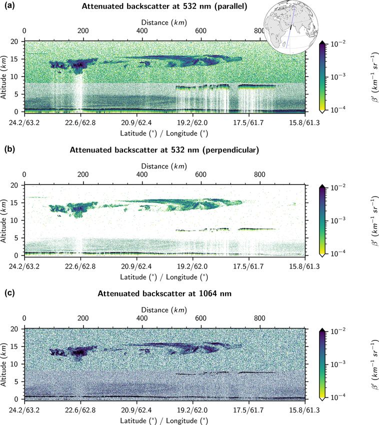
1594                                                                      T. Vaillant de Guélis et al.: 2D-McDA for CALIOP

   The critically important first step in retrieving the spatial      Section 2 presents a refined method for determining fea-
and optical properties of clouds and aerosols is to determine      ture detection thresholds, which are a critically important
where these “features” are located in the vertical, curtain-       component of the detection algorithm. Section 3 presents the
like images (altitude vs. satellite track) of the backscattered    detection algorithm. The detection of the Earth’s surface is
lidar signals (Fig. 1). The CALIPSO feature detection al-          described first as it is performed first and separately from the
gorithms were first developed for ground-based observa-            cloud and aerosol detection. This has been shown to have
tions and then adapted for space-based analyses using LITE         many practical advantages. Then, the cloud and aerosol de-
measurements and CALIPSO simulations. These algorithms,            tection algorithm is described. Finally, the detections from
which were conceived more than 25 years ago (e.g., Winker          each channel are merged into a composite feature detection
and Vaughan, 1994), at a time when computational power             mask. Section 4 shows how this new algorithm improves the
was considerably lower than what is now available, are in-         feature detection compared to the CALIPSO version 4 verti-
voked sequentially on single, one-dimensional (1-D) lidar          cal feature mask (VFM).
signal profiles (possibly generated from averaging data from
several consecutive laser pulses). Moreover, in order to min-
imize the computational load, the current CALIPSO algo-            2   Threshold-based feature detection
rithm is only applied to the 532 nm total signal (Vaughan
                                                                   Atmospheric lidars measure attenuated signal backscattered
et al., 2009).
                                                                   by molecules (m) and particles (p):
   To locate cloud and aerosol layers within lidar backscat-
ter profiles, two main approaches are generally employed:          β 0 (r) = βm (r) + βp (r) Tm (r)2 TO3 (r)2 Tp (r)2 ,

                                                                                                                          (1)
the slope-based method, which looks for zero crossings in
the first derivative of the raw signal (e.g., Pal et al., 1992)    where βm (r) and βp (r) are the volume backscatter coeffi-
and threshold-based methods, which search for regions ex-          cients for molecules and particulates, and Tm (r)2 , TO3 (r)2
ceeding some expectation of the maximum signal value that          and Tp (r)2 are, respectively, the two-way transmittances for
could be measured in “clear air” (e.g., Winker and Vaughan,        molecules, ozone and particles, and r is the range from the
1994; Clothiaux et al., 1998; Campbell et al., 2008). Some         satellite altitude. If there are no particles in the atmosphere,
studies use a combination of both methods (e.g., Wang and          Eq. (1) reduces to the molecular attenuated backscatter coef-
Sassen, 2001; Lewis et al., 2016). A few others adopt a            ficient:
third method: the wavelet analysis (e.g., Davis et al., 2000;
Brooks, 2003). Because these layer detection algorithms are
                                                                    0
                                                                   βm (r) = βm (r)Tm (r)2 TO3 (r)2 .                           (2)
applied successively to individual 1-D profiles (either single
                                                                      A feature, i.e., a cloud or an aerosol layer, appears as
shot or averaged), we define them collectively as “profile-
                                                                   an extended and contiguous region of enhanced attenuated
based processes”. We also define a second, more comprehen-
                                                                   backscatter signal that rises significantly above the expected
sive class of methods as “scene processes”. Scene processes
                                                                   clear-sky (molecules only) value. However, not all signals
can take advantage of the contextual information provided
                                                                   that exceed the expected values of β \0
by a continuous series of profile measurements by searching                                              m (r) necessarily indicate
for cloud and aerosol patterns in the two-dimensional (2-D)        the presence of features; instead, such excursions are often
image formed by successive lidar profiles. While edge de-          caused by noise. To distinguish features from the ambient
tection techniques based on 2-D gradient search routines are       (but noisy) clear-sky signals, a first step is to determine a
not well suited for spatial analysis of lidar data (Vaughan        threshold above which signals can be confidently attributed
et al., 2005), methods based on sliding window operations          to enhanced scattering arising from clouds or aerosols. We
have been shown to greatly improve the feature shape detec-        construct this threshold by first calculating the expected
                                                                   molecular attenuated backscatter, β  \0
tion (e.g., Hagihara et al., 2010; van Zadelhoff et al., 2011;                                           m (r), to which we add k
Herzfeld et al., 2014).                                            times the expected noise-induced standard deviation of the
   Here, we propose a new 2-D and multi-channel feature de-        molecular signal. The resulting range-dependent threshold
tection algorithm (2D-McDA). This “context-sensitive” fea-         is the sum of β\0
                                                                                   m (r) and, based on error propagation theory
ture finder algorithm is then applied to a 2-D lidar sig-          (e.g., Bevington and Robinson, 2003), k times the root mean
nal scene, i.e., to the image formed by many successive li-        square (rms) of the standard deviations due to both range-
dar profiles. Moreover, the 2-D detection algorithm uses the       independent and range-dependent noise sources.
backscatter signals from all available channels: the 532 nm           In constructing thresholds to be applied to CALIOP data,
co-polarized (or parallel) signal, the 532 nm cross-polarized      one must take into account the onboard signal averaging
(or perpendicular) signal and the 1064 nm signal. Since the        that is applied to the backscatter measurements. Because
backscatter from some aerosol or cloud particle types can          the CALIPSO satellite has limited telemetry bandwidth, the
be more pronounced in one channel than another, simultane-         backscatter data are averaged both vertically and horizontally
ously assessing the signals from all channels is expected to       before the data are downlinked from the satellite, with in-
greatly improve the layer detection.                               creasing amounts of averaging applied to data acquired at

Atmos. Meas. Tech., 14, 1593–1613, 2021                                             https://doi.org/10.5194/amt-14-1593-2021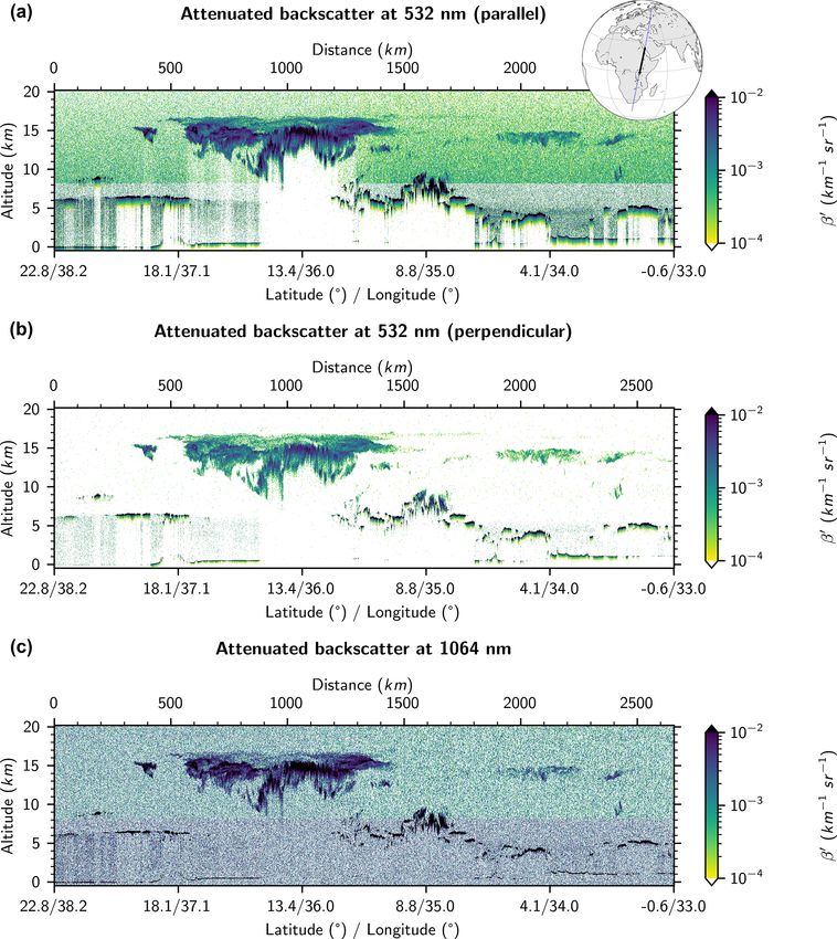
T. Vaillant de Guélis et al.: 2D-McDA for CALIOP                                                                                   1595

Figure 1. Curtain of attenuated backscatter signal measured by CALIOP in the 532 nm parallel channel during nighttime observations on
31 August 2018, 21:46:37 UTC (start point), over the Arabian Sea.

higher altitudes (Hunt et al., 2009). As an example, signals
acquired between 8.2 and 20.2 km are averaged horizontally
over three consecutive lidar pulses and vertically for four
full-resolution (15 m) range bins. Consequently, the down-
linked profile data from within this region have been aver-
aged over 12 full-resolution onboard range bins. We com-
pute a range-dependent threshold specifically tailored for the
CALIOP profiles using
                                 r
                     fcorr (r)                           2
βT0 (r) = β
          \ 0
           m (r) + k √               1βb0 (r)2 + 1β
                                                  \ 0
                                                    m (r) ,   (3)
                        N (r)

where 1βb0 (r) is the standard deviation due to background
noise (range independent1 ), 1β \ 0
                                  m (r) is the expected standard
deviation due to the shot noise (range dependent) in the ex-
                                                                     Figure 2. Range-dependent threshold (red) applied to a single-shot
pected clear sky, and N (r) is the number of bins averaged on-       lidar signal profile (blue) in clear sky during nighttime. The esti-
board. The fcorr (r) term is a correction function which takes       mated molecular signal is shown in black. Jumps in the lidar signal
into account the partial vertical correlation in samples due to      and threshold at −0.5, 8.2 and 20.2 km reveal the change of onboard
the limited electronic bandwidth and the shifting and rebin-         averaging resolution.
ning that can occur in the altitude registration phase of the
level 1A processing (details in Appendix A). The number
of shot noise standard deviations considered in the thresh-
old is quantified by the factor k, which can be tuned accord-        The NSF is evaluated from the solar background signal
ing to the degree of sensitivity needed to avoid false detec-        during daytime for the 532 nm parallel and perpendicu-
        \0                                                           lar channels (Hostetler et al., 2006; Liu et al., 2006). At
tions. β m (r) is derived from modeled profiles of molecular         1064 nm, CALIOP uses an avalanche photodiode (APD) de-
and ozone number densities. 1βb0 (r) is derived from the on-
                                                                     tector rather than the photomultiplier tubes (PMTs) that are
board computation of the rms of the background signal in
                                                                     used for the 532 nm channels. Because the APD dark noise
the high-altitude background region (HABR) between 65 and
                                                    0
                                                                     overwhelms the 1064 nm shot noise, only the background
80 km for each shot (Hostetler et al., 2006). 1β  \
                                                    m (r) is esti-   noise is considered at 1064 nm.
mated using its proportional relation with the square root of           Figure 2 shows the range-dependent threshold (red) com-
\ 0
β m (r) (e.g., Liu and Sugimoto, 2002), called the “noise scale      puted from Eq. (3) with k = 2 applied to the 532 nm par-
factor” (NSF):                                                       allel lidar signal (blue) for a clear-sky case study during
                    q                                                nighttime. Note the noise due to the quantum nature of pho-
  \  0
1βm (r) = NSFβ 0 β    \ 0
                       m (r).                                 (4)    tons (shot noise) in this figure. Indeed, although background
                                                                     noise, mainly due to solar radiation, is quite low during night-
    1 The background noise is range- independent in the digitizer-   time, the lidar signal shows large variations around the ex-
reading domain P . However, it then depends on r when transformed    pected clear-sky return (black). The range-dependent thresh-
to the β 0 domain.                                                   old correctly keeps most the signal below the detection level.

https://doi.org/10.5194/amt-14-1593-2021                                                Atmos. Meas. Tech., 14, 1593–1613, 2021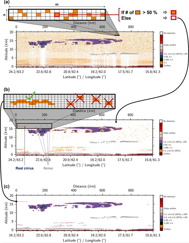
1596                                                                           T. Vaillant de Guélis et al.: 2D-McDA for CALIOP

                                                                        first an independent detection of the Earth’s surface. Doing
                                                                        the surface detection in a first and separate step allows a bet-
                                                                        ter retrieval of the surface echo and prevents complications in
                                                                        the cloud and aerosol layer detection process. Also, knowing
                                                                        where the surface is detected allows subsequent separation
                                                                        of semi-transparent features from opaque features, which is
                                                                        essential for accurately estimating range-resolved profiles of
                                                                        extinction coefficients (Young et al., 2018). Operationally,
Figure 3. Pixels of Fig. 1 where the lidar signal is above the range-
                                                                        atmospheric features are defined as being opaque when no
dependent threshold computed from Eq. (3) with k = 2 are shown          surface return or other atmospheric feature can be detected
in orange. Brown pixels show surface detection.                         below them. From this definition, it follows that the signals
                                                                        received from beneath opaque features have been fully at-
                                                                        tenuated within these features. The Earth surface detection
Jumps at −0.5, 8.2 and 20.2 km reveal the change of onboard             algorithm used here is closely akin to the one described in
averaging resolution. However, a few points of the lidar sig-           Vaughan et al. (2021) and is applied to the 532 nm paral-
nal still exceed the threshold. Some continuity tests are then          lel and 1064 nm channels (details in Appendix B). The sig-
needed to determine whether these high signals are due to               nals from the top of the detected surface echo and below this
noise or instead part of an extended feature. Unlike the cur-           point are removed from the data. To minimize computation
rent CALIPSO detection algorithm, this continuity test will             times, the surface detection algorithm is not applied to the
be applied in two dimensions. Figure 3 shows all pixels of              532 nm perpendicular channel signal. The backscatter from
Fig. 1 where the lidar signal is above the range-dependent              ocean surfaces (covering ∼ 70 % of the planet) does not de-
threshold computed from Eq. (3) with k = 2.                             polarize and, excluding snow and ice, the depolarization of
   Like the current CALIOP layer detection algorithm, the               most land surfaces is relatively low (Lu et al., 2017); hence,
2D-McDA is applied to profiles of attenuated scattering ra-             the preponderance of the surface backscatter is in the paral-
tios, defined as                                                        lel channel. The altitude retrieved in the parallel channel is
            β 0 (r)                                                     used to remove the signal at and below the estimated surface
R 0 (r) =    0 (r)
                    .                                            (5)    altitude in the perpendicular channel. Note that there is some
            βm
                                                                        small chance that a surface echo can appear in the perpen-
The attenuated scattering ratio threshold is then obtained              dicular channel but not be visible or detected in the parallel
from                                                                    channel. The detection of the surface corresponding to Fig. 1
         β 0 (r)                                                        is shown in brown in Fig. 3.
RT0 (r) = T
         \
         β 0 (r)
               m                                                        3.2   Cloud and aerosol detection
                         v
               fcorr (r) u 1                             1
                         u
         = 1+k √         t      2
                                  1βb0 (r)2 + NSF2β 0        .   (6)    The detection of cloud and aerosol layers in a single channel
                 N(r) β    0 (r)
                           \                          \0
                                                      βm (r)
                             m                                          curtain of lidar measurements takes place in four main steps:
  Equation (6) is applied to the three lidar channels (532 nm
                                                                         1. detecting strong features, i.e., identifying contiguous re-
parallel, 532 nm perpendicular and 1064 nm) during the 2D-
                                                                            gions of enhanced attenuated scattering ratios that rise
McDA process.
                                                                            above the feature detection threshold (which is repeat-
                                                                            edly decreased from a very large value of k down to k =
3     2-D and multi-channel feature detection algorithm                     1) without applying any signal averaging (i.e., d = 1–4
                                                                            in Table 1, Sect. 3.2.1);
The 2D-McDA is applied to the scattering ratio signals at
532 nm parallel, 532 nm perpendicular and 1064 nm. First,                2. flagging regions below opaque features as “fully attenu-
the detection of the surface altitude is performed and the sig-             ated” (FA) and regions below transparent features where
nal from this altitude and below is removed from the data.                  the signal is strongly attenuated with the low confidence
Second, the detection of cloud and aerosol layers is done in                flag “almost fully attenuated” (AFA) (Sect. 3.2.2);
each channel based on iterated detection thresholds and 2-
D spatial continuity tests. Finally, the masks from the three            3. averaging of those signals not already flagged using a
channels are merged in a composite feature mask.                            horizontal sliding window (Sect. 3.2.3); and

3.1    Surface detection                                                 4. detecting faint features; features are once again identi-
                                                                            fied as contiguous regions of enhanced signal (i.e., av-
Before detecting cloud and aerosol layers using the detection               eraged attenuated scattering ratios) that rise above the
threshold as described in the previous section, we perform                  recomputed feature detection threshold (Sect. 3.2.1).

Atmos. Meas. Tech., 14, 1593–1613, 2021                                                  https://doi.org/10.5194/amt-14-1593-2021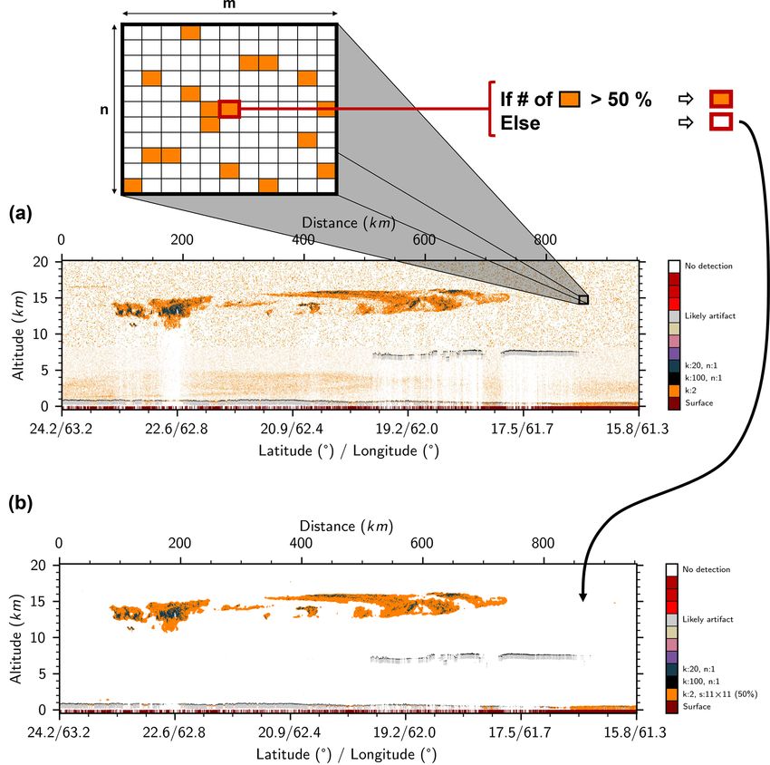
T. Vaillant de Guélis et al.: 2D-McDA for CALIOP                                                                                       1597

Figure 4. Flowchart of the two-dimensional and multi-channel feature detection algorithm (2D-McDA). d is the detection step, k is the
number of total noise standard deviations used in the detection threshold Eq. (3), s is the size of the window used for the spatial coherence
test, n is the minimum number of pixels in each pattern, and a is the size of the averaging window. See the algorithm description in Sect. 3
and the coefficient values in Table 1.

   Figure 4 shows the flowchart of the whole detection algo-             standard deviation with k = 2 (Fig. 5a; orange pixels). Then,
rithm. The parameter values used at the different detection              the second substep is to apply a spatial coherence test win-
levels are given in Table 1.                                             dow (rows a in Table 1) on these detected pixels (Fig. 5a, b).
   The following subsections give the details of the main                Here, an 11 × 11 pixels window is applied to each pixel of
steps presented above.                                                   the image, with the window being centered successively on
                                                                         all pixels. If the number of originally detected pixels in the
3.2.1   Detection                                                        window is greater than half of the total number of pixel in the
                                                                         window (≥ 61 for a 11 × 11 pixels window), then the center
The detection phase is performed following three substeps:               pixel is considered to be detected. If not, the center pixel is
  1. All pixels within the image that exceed the threshold are           considered to be undetected. In this smoothing step, the de-
     first flagged as detected (Fig. 3).                                 termination of detection status does not rely on a single pixel
                                                                         exceeding its threshold but instead on the fraction of neigh-
  2. A spatial coherence test window is applied to the im-               boring pixels that exceed their thresholds. Consequently, a
     age of detected versus undetected pixels. It smooths the            pixel classified as detected may not itself exceed the de-
     shape of detected pattern and removes isolated noisy de-            tection threshold. Similarly, a pixel that exceeds the thresh-
     tected pixels by turning some of detected pixels to un-             old may not ultimately be classified as detected. The pixel
     detected or undetected to detected.                                 count within the window is limited to those detected at the
  3. Smoothed patterns are required to meet a minimum nu-                current detection level d and at the previous detection level
     meric threshold of contiguous pixels. Patterns that fail            d − 1. This allows detection continuity of similar backscatter
     to meet this threshold are removed from consideration               intensities and avoids connecting noise encountered during
     for this level of detection.                                        fainter detections to a strong feature detected earlier. Other
                                                                         flagged pixels (i.e., “surface”, detection ≤ d − 2, “likely arti-
   The scattering ratio image used in the layer detection                fact”, “fully attenuated”, “almost fully attenuated” and “low
scheme has a spatial resolution of one laser pulse horizon-              confidence small strips” (to be described in detail later in
tally and 30 m vertically, equivalent to the finest spatial res-         this section and Sect. 3.2.2) and pixels outside the window
olution of the CALIOP data. As described in Hunt et al.                  when the top or bottom edges of the image are not consid-
(2009), CALIOP data are averaged aboard the satellite with               ered in the window and the total number of candidate pix-
spatial resolutions that vary according to altitude. Scattering          els in the window is decreased accordingly. The shapes of
ratios in regions where the data resolution is coarser than              detected features are smoothed by the spatial coherence test
the image resolution (30 m × 0.33 km horizontally) are du-               window, while the noise (isolated orange pixel) is removed.
plicated as necessary to match the image resolution. For ex-             However, some small clusters of pixels sometimes persist.
ample, between 8.2 and 20.2 km, the spatial resolution of the            Those small clusters cannot be confidently declared as fea-
signal is 1 km horizontally ×60 m vertically. These values               tures at this stage. They can be due to noise or they can be
are replicated 12 times to populate the corresponding area               part of a larger, fainter feature. Then, we decide not to con-
in the 30 m × 0.33 km scattering ratio image. The first sub-             sider these small patterns as detected features and retain these
step is then to flag all pixels of this image which exceed the           regions for inclusion in the signal averaging used in succes-
detection threshold given by Eq. (6) with the value of k de-             sive iterations of the algorithm. To be declared as detected
fined in Table 1. For example, for the 532 nm parallel chan-             features, smoothed detected patterns need to consist of more
nel, at the detection level d = 3, the detected pixels are those
where the signal is greater than 1+k times the expected noise

https://doi.org/10.5194/amt-14-1593-2021                                                    Atmos. Meas. Tech., 14, 1593–1613, 2021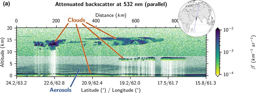
1598                                                                            T. Vaillant de Guélis et al.: 2D-McDA for CALIOP

Table 1. Coefficient k in threshold detection, spatial coherence test window size s, minimum number of pixels in pattern n and averaging
window size a used at each detection level d. Window sizes are given in vertical × horizontal pixel counts, with a single pixel resolution of
30 m × 0.33 km.

                                 d                 1      2              3                  4                  5
                                             k    100    20              2                  1                  1
                                             s     –      –          11 × 11              3 × 21             9 × 51
                        532 nm parallel                         (330 m × 3.67 km)     (90 m × 7 km)     (270 m × 17 km)
                                             n     1      1             60                 200               10 000
                                             a     –      –              –                  –                1 × 15
                                                                                                         (30 m × 5 km)
                                             k    500    100             2                  1                  1
                                             s     –      –          11 × 11              3 × 21             9 × 51
                    532 nm perpendicular                        (330 m × 3.67 km)     (90 m × 7 km)     (270 m × 17 km)
                                             n     1      1             60                 200               1000
                                             a     –      –              –                  –                1 × 15
                                                                                                         (30 m × 5 km)
                                             k     –     20              2                  1                  1
                                             s     –      –          11 × 11              3 × 21             9 × 51
                           1064 nm                              (330 m × 3.67 km)     (90 m × 7 km)     (270 m × 17 km)
                                             n     –      1             60                 200               10 000
                                             a     –      –              –                  –                1 × 15
                                                                                                         (30 m × 5 km)

than n connected pixels (see Table 1); otherwise, they are re-           initial scan is to identify the tops of very strongly scattering
moved from this detection level.                                         liquid clouds and ice clouds containing high fractions of hor-
   This detection procedure is applied several times (the suc-           izontally oriented ice (HOI) crystals. The non-ideal transient
cessive detection level d of Table 1) with different thresholds,         response by PMTs following these very strong signals often
different spatial coherence test windows s and different lim-            generates a spurious, exponentially decaying signal enhance-
its on the number of connected pixels required n (Table 1) in            ment in the underlying range bins (McGill et al., 2007; Hunt
order to detect all layers from the most evident, very strong            et al., 2009; Lu et al., 2020). The presence of these “noise
patterns to the very faint ones and from geometrically small             tails” in the 532 nm signals can introduce large biases into the
patterns to very extended ones. Note that the horizontal spa-            determination of the apparent bases of opaque water clouds.
tial coherence test window (3 × 21) enables the detection of             To exclude this artifact in the detection process, the 600 m
faint but horizontally extended cirrus such as the layer shown           below the base of the detected very strong signal are flagged
between 50 and 100 km in Fig. 1. The detection of this sub-              as “likely artifact” and removed from the signal. Since the
visible cirrus is presented in Fig. 6. Figure 6a–b show the              APD used in 1064 nm channel does not produce these noise
implementation of the 3 × 21 spatial coherence test window.              tails, we rely on the 1064 nm channel for the detection of the
We see that the cirrus pattern is smoothed and now clearly ap-           apparent base of these strongly scattering layers.
pears in Fig. 6b due to the fact that most of the noise around              After detection of the strongest features, i.e., without sig-
has been removed. However, many small clusters of noise                  nal averaging (d = 1 − 4 in Table 1), we flag all pixels below
pixels persist. By applying the minimum numeric threshold                a detected strong feature where the surface has not been de-
of connected pixel n on the detected pattern, we are able to             tected as “fully attenuated” (FA). In this portion of the pro-
remove small clusters due to noise while keeping the real cir-           file, the signal is too weak to be further exploited. Second,
rus (Fig. 6c).                                                           the contiguous pixels located in the vertical extent between
                                                                         two detected features are flagged as “almost fully attenuated”
3.2.2   Special flags                                                    (AFA) whenever the backscatter intensity falls below an em-
                                                                         pirically determined threshold. For the 532 nm parallel chan-
For the 532 nm channels, a first detection of a very strong              nel, these pixels are flagged as AFA when more than 30 %
signal is performed (see d = 1 in Table 1). The aim of this

Atmos. Meas. Tech., 14, 1593–1613, 2021                                                    https://doi.org/10.5194/amt-14-1593-2021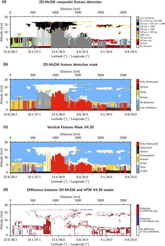
T. Vaillant de Guélis et al.: 2D-McDA for CALIOP                                                                                          1599

Figure 5. Illustration of the spatial coherence test window substep of 2D-McDA on the 532 nm parallel channel for the case study shown in
Fig. 1. (a) Pixels which are over the detection threshold given by Eq. (6) with the value of k = 2 (orange). (b) Result after applying a 11×11
spatial coherence test window on the detected pixels. Note that the insert at the top is just an illustration and does not show the real content
of the image portion.

of the population has backscatter intensities that are less than            After removing all data identified with these low confi-
10 % of the corresponding detection thresholds. These pix-                dence flags from the attenuated scattering ratios, the signal is
els are flagged as AFA in the 532 nm perpendicular channel                averaged in order to try to detect fainter features.
whenever the signals in more than 90 % of the population
fall below (100 % of) the corresponding threshold values. To              3.2.3    Signal averaging
be flagged as AFA in the 1064 nm channel, more than 85 %
of the population must have a signal less than (100 %) of                 We then average the remaining signal (here the attenuated
the corresponding threshold. In all cases, the AFA thresholds             scattering ratios) using a Gaussian sliding window that ex-
were determined experimentally and are tunable. Finally, the              tends over 5 km (15 profiles) horizontally and a single range
horizontal distance between successive (A)FA columns can                  bin vertically (a in Table 1). Using a sliding window, instead
be very small and the likelihood of confidently detecting fea-            of the fixed window used in the CALIOP feature detection al-
tures in these narrow gaps is very low. For this reason, the              gorithm, provides much improved resolution of the horizon-
data in all horizontal extents smaller than 5 km (15 profiles)            tal edges’ position of faint features (0.33 km instead of 5, 20,
that lie between (A)FA columns are flagged as “low confi-                 or 80 km) and makes it possible to detect non-uniform hor-
dence small strips”.                                                      izontal edges. A Gaussian weight with a standard deviation
                                                                          of 1.67 km is applied, thus giving a stronger weight to pixels
                                                                          closer to center of the window than at the edges. We chose
                                                                          a horizontal window here because the spatial extent of very

https://doi.org/10.5194/amt-14-1593-2021                                                      Atmos. Meas. Tech., 14, 1593–1613, 2021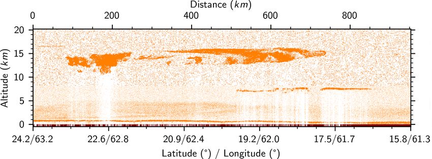
1600                                                                                T. Vaillant de Guélis et al.: 2D-McDA for CALIOP

Figure 6. Illustration of the horizontal spatial coherence test window substep and the pattern size threshold rejection substep of 2D-McDA
on the 532 nm parallel channel for the case study shown in Fig. 1. (a) Pixels which are over the detection threshold given by Eq. (6) with
the value of k = 1 (orange). (b) Result after applying a 3 × 21 spatial coherence test window on the detected pixels. (c) Result after rejecting
all patterns composed by less than n = 200 pixels (note that the insert at the top is just an illustration and does show the real content of the
image portion). Before these substeps, surface is detected first (brown); then, a very strong signal (k = 100) occurring on highly reflecting
liquid clouds is detected (black) and the 600 m below is flagged as “likely artifact” (gray), as it is the region where we see artifacts due to the
time response of photomultiplier tubes (PMTs) in the 532 nm channels. Two detections were also made: one with k = 20 and another with
k = 2, a 11 × 11 spatial coherence test window and n = 60.

faint layers is mainly in the horizontal direction. Typically,              Pixels flagged as surfaces or features are not considered in
thin cirrus have geometrical thicknesses of a few hundreds of               the averaging window. However, if the center pixel of the av-
meters but spread horizontally over several hundreds of kilo-               eraging window (i.e., the pixel to which the averaging is ap-
meters. The use of a horizontal averaging window thus al-                   plied) is a low confidence pixel (i.e., “likely artifact”, (A)FA
lows the detection of thin layers close to each other vertically.           or “low confidence small strips”), then the averaging window

Atmos. Meas. Tech., 14, 1593–1613, 2021                                                        https://doi.org/10.5194/amt-14-1593-2021
T. Vaillant de Guélis et al.: 2D-McDA for CALIOP 1601
Figure 7. Final feature mask of the 532 nm parallel channel.
is applied, and, if the average signal value exceeds the detec- sponse artifacts (note that the light blue color indicates “1064
tion threshold, this center pixel in the feature detection mask only” in Fig. 9a).
is “unflagged” until the end of the detection-level processing,
after which its low confidence flag is restored. This allows
us to maintain connections between features separated by a 4 Performance assessments and comparisons to
few low confidence pixels. Once the averaging is performed, version 4
the detection substeps (Sect. 3.2.1) are then applied to the
averaged signal. Note too that horizontally adjacent features In this section, we present two case studies to show the im-
separated only by a low confidence vertical band (i.e., pix- provements made by this new feature detection approach.
els classified as FA, AFA and/or small strips) are considered
4.1 Variety of cloud type and shape
a single, merged feature when counting the number of con-
nected pixels. Some examples of this horizontal merging are Figure 10 presents the attenuated backscattered lidar signal
seen in the smaller fragments of the aerosol layer found at in the three channels for another case study showing a vari-
about 4 km and an along-track distance of 500 km to 750 km ety of cloud types and shapes which occurred above Ethiopia
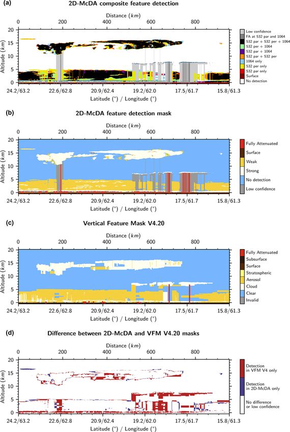
in Fig. 7. on 31 August 2018 during nighttime. We can see that the
Figure 7 shows the final mask for the 532 nm parallel chan- artifacts below liquid water clouds (close to the surface and
nel after the detection of the faint features. up to 8 km) appear in the 532 nm parallel (Fig. 10a) and the
532 nm perpendicular (Fig. 10b) channels but not at 1064 nm
3.3 Three-channel composite detection (Fig. 10c). We note that thin cirrus clouds, like the one at
17 km in altitude between 1550 and 1850 km, are clearly
The detection algorithm is applied individually to the lidar brought out in the 532 nm perpendicular channel (Fig. 10b).
signal from each of the three channels (Fig. 8), and all pix- If we look now at the composite feature detections derived
els identified as features in any of the three channels are re- from these three signals (Fig. 11a), we note again how well
tained in the composite mask (Fig. 9a). Comparing this new the apparent bases of liquid clouds are retrieved by using the
feature mask (Fig. 9a, b) to the current version of the VFM 1064 nm channel. We note also that the successful identifica-
(Fig. 9c), we first note the improvement in the detected con- tion of thin cirrus can largely be attributed to our use of the
tour of the large cirrus. We also note that the 2D-McDA read- 532 nm perpendicular channel. Figure 11b shows the same
ily detects faint cirrus (e.g., as seen between 0 and 75 km) mask as Fig. 11a but with the same colors that are used for the
that is missed by the current VFM. The vertical spreading VFM images (Fig. 11c). This change of colors is intended to
of the clouds seen in the VFM at around 7.5 km in altitude facilitate one-to-one comparisons between the two detection
and between 500 and 900 km horizontally is due to the afore- schemes. However, note that the yellow and white colors do
mentioned PMT artifact afflicting the 532 nm signals beneath not discriminate aerosol from cloud, as in the VFM, but in-
strongly scattering layers. This is not seen in the 2D-McDA stead simply differentiate weak from strong features based on
feature mask because pixels below the cloud top are flagged whether the feature detection required data averaging (yel-
as “likely artifact” in the 532 nm channels and so we make low) or not (white). Finally, Fig. 11d shows the difference
no attempt to retrieve the cloud apparent base of such opaque between the new composite feature detection mask and the
clouds at this wavelength. Instead, in these cases, we retrieve VFM. We see that the contour of features retrieved by the 2D-
the true penetration depth estimates using the 1064 nm sig- McDA represents a distinct improvement over the squared
nals (Fig. 8c), which are not affected by detector transient re- boundaries reported by the VFM. We note too that the new
https://doi.org/10.5194/amt-14-1593-2021 Atmos. Meas. Tech., 14, 1593–1613, 2021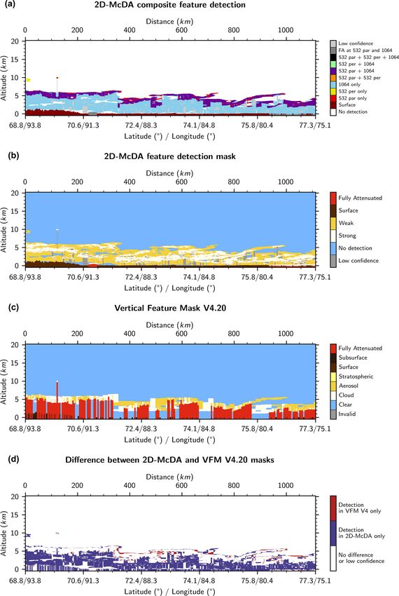
1602 T. Vaillant de Guélis et al.: 2D-McDA for CALIOP
Figure 8. Curtain of attenuated scattering ratios measured by CALIOP during nighttime observations on 31 August, 21:46:37 UTC (start
point), daytime observations at (a) 532 nm parallel (same as Fig. 1), (b) 532 nm perpendicular and (c) 1064 nm.
algorithm detects thin clouds that are obviously missed by cates that the signals are fully attenuated after detecting (at
the VFM and that it eliminates significant detection artifacts 532 nm) the apparent base of the smoke layer. However, at
reported by the VFM between 700 and 900 km. 1064 nm, the dense smoke layer is semi-transparent because
the 1064 nm signals are attenuated significantly less than at
4.2 Dense smoke 532 nm. Then, the surface is readily detected at 1064 nm
(Fig. 12c). This scene clearly illustrates the advantage gained
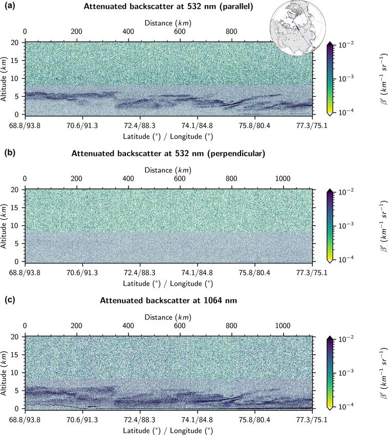
Figure 12 presents a dense smoke event in Siberia on 26 July by using a multi-channel feature detection algorithm, since
2006 during daytime. the full vertical extent of the smoke plume can only be re-
The smoke layer is opaque at 532 nm, and thus we do not trieved by inspecting the 1064 nm measurements (light blue
see any surface echo for this channel (Fig. 12a). Note that the color in Fig. 13a).
smoke is non-depolarizing so there is no perpendicular sig-
nal (Fig. 12b). Because the standard CALIOP layer detection
only examines the 532 nm channel, the VFM (Fig. 13c) indi-
Atmos. Meas. Tech., 14, 1593–1613, 2021 https://doi.org/10.5194/amt-14-1593-2021T. Vaillant de Guélis et al.: 2D-McDA for CALIOP 1603 Figure 9. (a) Composite feature detection mask derived from signals shown in Fig. 8. (b) Same as panel (a) but using the same colors as those used for the VFM. “Strong” (white) features are those detected without averaging in at least one channel; others are flagged as “weak” (yellow). (c) VFM of version 4 of the CALIOP data product. (d) Difference between the new mask and the VFM. https://doi.org/10.5194/amt-14-1593-2021 Atmos. Meas. Tech., 14, 1593–1613, 2021
1604                                                                      T. Vaillant de Guélis et al.: 2D-McDA for CALIOP

Figure 10. Curtain of attenuated scattering ratios measured by CALIOP during nighttime observations on 31 August 2018, 23:25:54 UTC
(start point), over Ethiopia at (a) 532 nm parallel, (b) 532 nm perpendicular and (c) 1064 nm.

5   Conclusions                                                     tails that are often obscured by CALIPSO’s standard multi-
                                                                    resolution averaging scheme. Relative to the CALIPSO ver-
                                                                    sion 4.2 vertical feature mask (VFM) data product, the 2D-
This paper describes the architecture and theoretical un-           McDA shows the following improvements.
derpinnings of a new two-dimensional, multi-channel fea-
ture detection algorithm (2D-McDA) used to identify layer             – Because it is applied to single profiles averaged over
boundaries in the backscatter signals acquired by the elas-             several different horizontal resolutions, the standard
tic backscatter lidar aboard the Cloud-Aerosol Lidar and                CALIOP feature detection produces blocky, rectangu-
Infrared Pathfinder Satellite Observations (CALIPSO) plat-              lar layers. The complex shapes of aerosol and cloud
form. The cloud and aerosol layer detection boundaries re-              features are better preserved by the 2D-McDA win-
ported in the standard CALIPSO data products are detected               dowing and data aggregation operations, which provide
by scanning sequences of 532 nm attenuated scattering ratio             the flexibility required to distinguish fine spatial details.
profiles constructed at increasingly coarser horizontal aver-           It is hoped that this improved feature detection will
aging resolutions. In contrast, the 2D-McDA is more akin to             lead to improvements in classifying features accord-
an image processing algorithm that examines full-resolution             ing to type (e.g., clouds vs. aerosols) and in their op-
lidar scenes and hence can identify many of the fine de-                tical property retrievals. Ideally, separate identification

Atmos. Meas. Tech., 14, 1593–1613, 2021                                              https://doi.org/10.5194/amt-14-1593-2021
T. Vaillant de Guélis et al.: 2D-McDA for CALIOP 1605 Figure 11. (a) Composite feature detection mask derived from signals shown in Fig. 10. (b) Same as panel (a) but using the same colors as those used for the VFM. “Strong” (white) features are those detected without averaging in at least one channel; others are flagged as “weak” (yellow). (c) VFM of version 4 of the CALIOP data product. (d) Difference between the new mask and the VFM. https://doi.org/10.5194/amt-14-1593-2021 Atmos. Meas. Tech., 14, 1593–1613, 2021
1606                                                                        T. Vaillant de Guélis et al.: 2D-McDA for CALIOP

Figure 12. Curtain of attenuated scattering ratios measured by CALIOP during a dense smoke event which occurred in Siberia on 26 July
2006, 06:00:25 UTC (start point), daytime observations at (a) 532 nm parallel, (b) 532 nm perpendicular and (c) 1064 nm.

     of strongly scattering and weakly scattering features by             thermal budget and drive dynamics of the tropopause
     the 2D-McDA will also offer improved discrimination                  region (e.g., Hartmann et al., 2001; McFarquhar et al.,
     between juxtaposed cloud and aerosol layers or identifi-             2000).
     able regions of ice and liquid water within a cloud. The
     improvement of the cloud shape detection is by itself             – The apparent base altitudes of highly reflective clouds,
     important, for example, for studies interested in anvil             i.e., the levels of complete attenuation of the lidar signal,
     clouds (e.g., Bony et al., 2016; Hartmann, 2016).                   which are routinely biased low (by several hundred me-
                                                                         ters) due to the non-ideal transient response of 532 nm
  – The detection of subvisible cirrus is significantly en-              photomultiplier tubes, are now more correctly retrieved
    hanced by both the 2-D detection scheme and the use of               by incorporating measurements made by the 1064 nm
    the 532 nm perpendicular channel, which is especially                channel. The apparent cloud base altitude, which re-
    sensitive to the presence of depolarizing ice crystals.              sults from both attenuation of the direct beam and mul-
    Those clouds play an important role in the climate sys-              tiple scattering effects, has been directly linked with
    tem as they regulate the vertical transport of water va-             the amount of longwave radiation escaping the Earth
    por near the upper troposphere–lower stratosphere (e.g.,             at the top of the atmosphere (Vaillant de Guélis et al.,
    Jensen et al., 1996; Luo et al., 2003), influence the local          2017a, b), making its accurate estimation very impor-

Atmos. Meas. Tech., 14, 1593–1613, 2021                                               https://doi.org/10.5194/amt-14-1593-2021
T. Vaillant de Guélis et al.: 2D-McDA for CALIOP 1607 Figure 13. (a) Composite feature detection mask derived from signals shown in Fig. 12. (b) Same as panel (a) but using the same colors as those used for the VFM. “Strong” (white) features are those detected without averaging in at least one channel; others are flagged as “weak” (yellow). (c) VFM of version 4 of the CALIOP data product. (d) Difference between the new mask and the VFM. https://doi.org/10.5194/amt-14-1593-2021 Atmos. Meas. Tech., 14, 1593–1613, 2021
1608                                                               T. Vaillant de Guélis et al.: 2D-McDA for CALIOP

     tant for cloud feedback studies (Vaillant de Guélis et al.,
     2018).
  – The 2D-McDA can retrieve the full vertical extent of
    dense smoke layers by examining the 1064 nm channel.
    Within smoke, the 1064 nm signals are attenuated sig-
    nificantly less than at 532 nm and hence can more often
    penetrate the full vertical extent of these layers. Those
    biomass burning aerosols play a significant role in the
    Earth’s radiative balance by their scattering and absorp-
    tion of incoming solar radiation (e.g., Penner et al.,
    1992; Christopher et al., 1996) and the interaction they
    have with clouds (e.g., Kaufman and Fraser, 1997). The
    full detection of those layers will lead to more accurate
    aerosol optical depth retrievals which will improve es-
    timates of the radiation budget. Profiling the full depth
    of the smoke layer will also help to understand whether
    the layer is in contact with underlying clouds and able
    to affect cloud microphysics.
While the current implementation of the algorithm is compu-
tationally intensive, numerous optimizations are underway,
and it is now feasible to apply the 2D-McDA operationally
using CALIPSO’s available computer resources. However,
while fundamentally important, feature detection is only the
first step in extracting a comprehensive suite of geophysical
parameters from raw lidar measurements. Taking full advan-
tage of the improved spatial analyses delivered by the 2D-
McDA thus requires the development of a companion set of
2-D scene processes to replace the 1-D profile-based pro-
cesses that are currently used in the CALIPSO retrieval ar-
chitecture to perform the essential tasks of discriminating be-
tween clouds and aerosols, identifying cloud thermodynamic
phase and classifying aerosols by type.

Atmos. Meas. Tech., 14, 1593–1613, 2021                                    https://doi.org/10.5194/amt-14-1593-2021
T. Vaillant de Guélis et al.: 2D-McDA for CALIOP 1609
Appendix A: Correction functions A2 Correction due to redistribution in altitude
registration
A1 Correction due to electronic bandwidth
An additional correlation arises from the data redistribution
A correction should be applied to Eq. (3) due to the fact in the altitude registration of level 0 data during the level 1A
that the nominal sample range interval (15 m) of the lidar processing. Indeed, the altitudes of the sample bins of a raw
is smaller than its range resolution (≈ 40 m) determined by data profile are recalculated with more accurate information
the electronic bandwidth (2 MHz; Hunt et al., 2009). Con- about the satellite altitude and laser viewing angle in the data
sequently, a 15 m sample bin is partially correlated with the processing on ground. A shift for a few range bins (no more
two bins above and the two bins below. As a result, vertical than three in most of the cases) can be needed for the full-
averaging of several 15 m bins Nbin does not reduce the noise resolution (30 m) samples. The number of 30 m bins shifted
standard deviation as much as it would if the samples were Nshift30 (which we express below in terms of an equivalent
independent. A function fa (Nbin ) > 1 is then applied to cor- number of 15 m bins shifted; Nshift15 ) only add correlation to
rect from this partial correlation. This function is evaluated regions in the profile data where the vertical range resolution
as follows. is coarser than 30 m, i.e., where the vertical range resolutions
A 15 m bin bi has a variance Var(bi ). If Nbin 15 m bins are are 60, 180 and 300 m (Winker et al., 2006). Indeed, in those
vertically averaged together to form a larger bin B, then the regions, a vertical shift by Nshift30 30 m bins led to the ne-
variance of the mean is given by cessity of rebinning two neighboring bins larger than 30 m
1 X Nbin which introduce additional correlation to those bins. When
Var(B) = Var bi there is a shift of Nshift15 15 m bins (an even number since
Nbin i=1 shifts are performed at 30 m resolution), each new shifted bin
Nbin Bk0 , with vertical resolution coarser than 30 m, is computed
1 X from the weighted average of the two original bins (with Nbin
= 2
Var bi
Nbin i=1 size resolution) it steps across (Bk and Bk+1 ; Fig. A1) follow-
Nbin ing
1 X
= Cov(bi , bj )
2
Nbin Nbin − Nshift15 Nshift15
i,j =1 Bk0 = Bk + Bk+1 , (A4)
Nbin
Nbin Nbin
1 X X
= 2 Var(bi ) + 2 Cov(bi , bj ) , (A1) where
Nbin i=1 1≤i1610 T. Vaillant de Guélis et al.: 2D-McDA for CALIOP
The variance of a Bk0 can be written as
Var(Bk0 )
Nbin − Nshift15 Nshift15
= Var Bk + Bk+1
Nbin Nbin
2
Nshift15 2
Nbin − Nshift15
= Var(Bk ) +
Nbin Nbin
Nbin − Nshift15 Nshift15
Var(Bk+1 ) + 2 Cov(Bk , Bk+1 )
Nbin Nbin
" 2 2 #
Nbin − Nshift15 Nshift15 Var(b)
= +
Nbin Nbin Nbin
Nbin − Nshift15 Nshift15 Var(b)
fa (Nbin )2 + 2 2
Nbin Nbin Nbin
Nbin
X Cov(bi , bNbin +j )
i,j =1
Var(b)
" #
Nbin − Nshift15 2 Nshift15 2
Var(b)
= +
Nbin Nbin Nbin
Nbin Figure A1. Scheme of redistribution in altitude registration.
Nbin − Nshift15 Nshift15 1 X
fa (Nbin )2 + 2
Nbin Nbin Nbin i,j =1
R(Nbin + j − i) zdsurf given by a digital elevation model (DEM). The width of
this region will vary according to surface type. Since we are
Var(b)
"
Nbin − Nshift15
2
Nshift15
2 # highly confident of the surface altitude over the ocean (where
= + zdsurf = 0), we will only search in a very narrow range of al-
Nbin Nbin Nbin
titudes for profiles measured over the ocean. On the other
fa (Nbin )2 hand, we are somewhat less confident of the DEM surface
Nbin
Nbin − Nshift15 Nshift15 X m altitudes reported over land and even much less confident
+2 R(m) over Greenland and Antarctica, so our search regions over
Nbin Nbin m=1 Nbin
land will be larger. The surface echo can be very weak due to
NX
bin −1
Nbin − m attenuation by aerosol and cloud layers above. Then, we try
+ R(Nbin + m) . (A7)
m=1
Nbin to detect even the weakest surface echo as long as it is sub-
stantially above background noise. This procedure is applied
It follows that the correction function to apply on the stan- at single-shot resolution only. For each shot, the method is
dard deviation to take into account both the vertical partial made up of the following steps:
correlation due to the electronic bandwidth and the redistri-
1. Compute rd surf , the estimated range of the surface, from
bution in altitude registration is
surf and the satellite altitude zsat .
zd
fcorr (Nbin , Nshift15 ) 2. Compute 1βb0 (rdsurf ), the standard deviation due to back-
"
Nbin − Nshift15 2
#
Nshift15 2 ground noise in the β 0 domain at the range rd surf .
= + fa (Nbin )2
Nbin Nbin 3. Compute isurfd , the bin index of the estimated surface al-
Nbin
Nbin − Nshift15 Nshift15 X m NX
bin −1 titude, i.e., when z(isurf
d ) is closest to zd
surf .
+2 R(m) +
Nbin Nbin N
m=1 bin m=1 4. Define isurf
d ± 1i, the range of the surface search region
1/2 according to the International Geosphere-Biosphere
Nbin − m
R(Nbin + m) . (A8) Programme (IGBP) classification of the surface type at
Nbin the lidar footprint:
a. If surface type is Water and zd
surf = 0, then 1i =
Appendix B: Surface detection
2(≡ 60 m).
The aim of this procedure is to detect a surface echo in the b. Otherwise, if surface type is Permanent-Snow, then
near-neighborhood region of the estimated surface altitude 1i = 17(≡ 510 m).
Atmos. Meas. Tech., 14, 1593–1613, 2021 https://doi.org/10.5194/amt-14-1593-2021T. Vaillant de Guélis et al.: 2D-McDA for CALIOP 1611
c. Otherwise, 1i = 5 (≡ 150 m).
5. Compute the derivatives of the lidar signal for bin index
range 289–578 (8.2 to −0.5 km):
0
β 0 − βi−1
0
dβ
= i . (B1)
dz i zi − zi−1
6. Determine zmin and zmax , the altitudes of the minimum
and maximum values of the derivatives in the surface
search region, and imin and imax , their respective bin in-
dices.
0 , the maximum signal magnitude lying
7. Determine βmax
between zmin and zmax .
8. Sequentially test the three following rules to determine
if we have identified a legitimate surface return:
a. zmin > zmax ;
b. imin −imax ≤ N with N = 2 for the 532 nm channels
and N = 4 for the 1064 nm channel;
0
c. βmax > 31βb0 (rd
surf ).
9. If all rules are passed, set surface bin index isurf follow-
ing these conditions:
0
a. if dβ 0
dz i −1 > 0 or βimin −1 ≤ 0, then isurf = imin ;
min
0
b. otherwise (i.e., dβ dz ≤ 0 and βi0min −1 > 0),
imin −1
isurf = imin−1 for the 532 nm channels and isurf =
imin−2 for the 1064 nm channel.
10. If surface detection arose in a profile (profile horizontal
index p) but not in the previous (p−1) and the following
(p + 1) profiles, then the surface detection is canceled if
d ± 1. This last step reduces the surface search
isurf 6 ∈ isurf
region for isolated surface detection to prevent false de-
tection in a very attenuated region.
https://doi.org/10.5194/amt-14-1593-2021 Atmos. Meas. Tech., 14, 1593–1613, 20211612 T. Vaillant de Guélis et al.: 2D-McDA for CALIOP
Data availability. The CALIPSO level 1 lidar profile prod- tion of Hydrometeor Returns in Micropulse Lidar Data, J. Atmos.
uct used throughout this study is publicly distributed by Ocean. Tech., 15, 1035–1042, https://doi.org/10.1175/1520-
the NASA Langley Research Center Atmospheric Science 0426(1998)0152.0.CO;2, 1998.
Data Center: https://www-calipso.larc.nasa.gov/products/ Davis, K. J., Gamage, N., Hagelberg, C. R., Kiemle,
CALIPSO_DPC_Rev4x92.pdf (last access: 5 February 2021, C., Lenschow, D. H., and Sullivan, P. P.: An Ob-
https://doi.org/10.5067/CALIOP/CALIPSO/LID_L1-Standard-V4- jective Method for Deriving Atmospheric Structure
10, Vaughan et al., 2020). from Airborne Lidar Observations, J. Atmos. Ocean.
Tech., 17, 1455–1468, https://doi.org/10.1175/1520-
0426(2000)0172.0.CO;2, 2000.
Author contributions. TVdG led the design of 2D-McDA and Hagihara, Y., Okamoto, H., and Yoshida, R.: Development of
wrote the manuscript. MAV and DMW provided the knowledge of a combined CloudSat-CALIPSO cloud mask to show global
the weaknesses of the previous detection algorithm and brought the cloud distribution, J. Geophys. Res.-Atmos., 115, D00H33,
main ideas to address them. ZL developed the correction function https://doi.org/10.1029/2009JD012344, 2010.
and contributed to discussion and feedback essential to the study. Hartmann, D. L.: Tropical anvil clouds and climate sen-
sitivity, P. Natl. Acad. Sci. USA, 113, 8897–8899,
https://doi.org/10.1073/pnas.1610455113, 2016.
Competing interests. The authors declare that they have no conflict Hartmann, D. L., Holton, J. R., and Fu, Q.: The heat
of interest. balance of the tropical tropopause, cirrus, and strato-
spheric dehydration, Geophys. Res. Lett., 28, 1969–1972,
https://doi.org/10.1029/2000GL012833, 2001.
Herzfeld, U. C., McDonald, B. W., Wallin, B. F., Neumann,
Acknowledgements. The authors are grateful to Brian Magill for
T. A., Markus, T., Brenner, A., and Field, C.: Algorithm
helping improving the runtime of the algorithm and to Kenneth
for Detection of Ground and Canopy Cover in Micropulse
Beaumont and Brian Getzewich for running the algorithm on the
Photon-Counting Lidar Altimeter Data in Preparation for the
cluster of the Atmospheric Science Data Center. Thibault Vaillant
ICESat-2 Mission, IEEE T. Geosci. Remote, 52, 2109–2125,
de Guélis’ research was supported by an appointment to the NASA
https://doi.org/10.1109/TGRS.2013.2258350, 2014.
Postdoctoral Program at the NASA Langley Research Center, ad-
Hostetler, C. A., Liu, Z., Reagan, J., Vaughan, M., Winker, D., Os-
ministered by Universities Space Research Association under con-
born, M., Hunt, W. H., Powell, K. A., and Trepte, C.: Lidar Level
tract with NASA.
I ATBD. Calibration and Level 1 Data Products, Algorithm The-
oretical Basis Document, NASA Langley Research Document
PC-SCI-201, 66 pp., available at: https://www-calipso.larc.nasa.
Review statement. This paper was edited by Ulla Wandinger and gov/resources/pdfs/PC-SCI-201v1.0.pdf (last access: 5 February
reviewed by two anonymous referees. 2021), 2006.
Huang, J., Fu, Q., Su, J., Tang, Q., Minnis, P., Hu, Y., Yi, Y.,
and Zhao, Q.: Taklimakan dust aerosol radiative heating derived
from CALIPSO observations using the Fu-Liou radiation model
References with CERES constraints, Atmos. Chem. Phys., 9, 4011–4021,
https://doi.org/10.5194/acp-9-4011-2009, 2009.
Bevington, P. R. and Robinson, D. K.: Data Reduction and Error Hunt, W. H., Winker, D. M., Vaughan, M. A., Powell, K. A., Lucker,
Analysis for the Physical Sciences, McGraw-Hill, New York, P. L., and Weimer, C.: CALIPSO Lidar Description and Per-
NY, USA, 3rd edn., 2003. formance Assessment, J. Atmos. Ocean. Tech., 26, 1214–1228,
Bony, S., Stevens, B., Coppin, D., Becker, T., Reed, K. A., https://doi.org/10.1175/2009JTECHA1223.1, 2009.
Voigt, A., and Medeiros, B.: Thermodynamic control of anvil Jensen, E. J., Toon, O. B., Pfister, L., and Selkirk, H. B.: Dehy-
cloud amount, P. Natl. Acad. Sci. USA., 113, 8927–8932, dration of the upper troposphere and lower stratosphere by sub-
https://doi.org/10.1073/pnas.1601472113, 2016. visible cirrus clouds near the tropical tropopause, Geophys. Res.
Brooks, I. M.: Finding Boundary Layer Top: Ap- Lett., 23, 825–828, https://doi.org/10.1029/96GL00722, 1996.
plication of a Wavelet Covariance Transform Kaufman, Y. J. and Fraser, R. S.: The effect of smoke parti-
to Lidar Backscatter Profiles, J. Atmos. Ocean. cles on clouds and climate forcing, Science, 277, 1636–1639,
Tech., 20, 1092–1105, https://doi.org/10.1175/1520- https://doi.org/10.1126/science.277.5332.1636, 1997.
0426(2003)0202.0.CO;2, 2003. Lewis, J. R., Campbell, J. R., Welton, E. J., Stewart, S. A.,
Campbell, J. R., Sassen, K., and Welton, E. J.: Elevated and Haftings, P. C.: Overview of MPLNET Version 3
Cloud and Aerosol Layer Retrievals from Micropulse Li- Cloud Detection, J. Atmos. Ocean. Tech., 33, 2113–2134,
dar Signal Profiles, J. Atmos. Ocean. Tech., 25, 685–700, https://doi.org/10.1175/JTECH-D-15-0190.1, 2016.
https://doi.org/10.1175/2007JTECHA1034.1, 2008. Liu, Z. and Sugimoto, N.: Simulation study for cloud
Christopher, S. A., Kliche, D. V., Chou, J., and Welch, R. M.: First detection with space lidars by use of analog detec-
estimates of the radiative forcing of aerosols generated from tion photomultiplier tubes, Appl. Opt., 41, 1750–1759,
biomass burning using satellite data, J. Geophys. Res.-Atmos., https://doi.org/10.1364/AO.41.001750, 2002.
101, 21265–21273, https://doi.org/10.1029/96JD02161, 1996. Liu, Z., Hunt, W., Vaughan, M., Hostetler, C., McGill, M., Powell,
Clothiaux, E. E., Mace, G. G., Ackerman, T. P., Kane, T. J., Spin- K., Winker, D., and Hu, Y.: Estimating random errors due to shot
hirne, J. D., and Scott, V. S.: An Automated Algorithm for Detec-
Atmos. Meas. Tech., 14, 1593–1613, 2021 https://doi.org/10.5194/amt-14-1593-2021You can also read