HIRM v1.0: a hybrid impulse response model for climate modeling and uncertainty analyses - GMD
←
→
Page content transcription
If your browser does not render page correctly, please read the page content below
Geosci. Model Dev., 14, 365–375, 2021
https://doi.org/10.5194/gmd-14-365-2021
© Author(s) 2021. This work is distributed under
the Creative Commons Attribution 4.0 License.

HIRM v1.0: a hybrid impulse response model for
climate modeling and uncertainty analyses
Kalyn Dorheim, Steven J. Smith, and Ben Bond-Lamberty
Joint Global Change Research Institute, Pacific Northwest National Laboratory, College Park,
MD 20740, United States of America

Correspondence: Kalyn Dorheim (kalyn.dorheim@pnnl.gov)

Received: 31 January 2020 – Discussion started: 27 April 2020
Revised: 2 September 2020 – Accepted: 26 November 2020 – Published: 22 January 2021

Abstract. Simple climate models (SCMs) are frequently             1   Introduction
used in research and decision-making communities because
of their flexibility, tractability, and low computational cost.   Climate models encompass a diverse collection of ap-
SCMs can be idealized, flexibly representing major climate        proaches to representing Earth system processes at various
dynamics as impulse response functions, or process-based,         levels of complexity and resolution. The most complex are
using explicit equations to model possibly nonlinear climate      the Earth System Models (ESMs): highly detailed represen-
and Earth system dynamics. Each of these approaches has           tations of the physical, chemical, and biological processes
strengths and limitations. Here we present and test a hybrid      governing the Earth system at high spatial and temporal res-
impulse response modeling framework (HIRM) that com-              olution (Hurrell et al., 2013). These models are computation-
bines the strengths of process-based SCMs in an idealized         ally expensive and therefore can only be run for a limited
impulse response model, with HIRM’s input derived from            number of scenarios. Slightly less complex and more com-
the output of a process-based model. This structure enables       putationally efficient are the Earth System Models of Inter-
the model to capture some of the major nonlinear dynam-           mediate Complexity (EMICs) (Stocker, 2011). Finally, Sim-
ics that occur in complex climate models as greenhouse gas        plified Climate Models (SCMs) sacrifice process realism but
emissions transform to atmospheric concentration to radia-        are computationally inexpensive (van Vuuren et al., 2011).
tive forcing to climate change. As a test, the HIRM frame-        Although SCMs are generally low resolution in space and
work was configured to emulate the total temperature of the       time, they have a wide range of applications, including em-
simple climate model Hector 2.0 under the four Represen-          ulation (Dorheim et al., 2020a), probabilistic estimates de-
tative Concentration Pathways and the temperature response        manding thousands of separate model runs (Stainforth et al.,
of an abrupt 4 times CO2 concentration step. HIRM was able        2005; Webster et al., 2012), factor separation analysis (Meehl
to reproduce near-term and long-term Hector global temper-        et al., 2007), and Earth system model development and diag-
ature with a high degree of fidelity. Additionally, we con-       nosis (Meinshausen et al., 2011).
ducted two case studies to demonstrate potential applications        SCMs vary in complexity. Process-based SCMs such as
for this hybrid model: examining the effect of aerosol forcing    Hector (Hartin et al., 2015) and MAGICC (Meinshausen et
uncertainty on global temperature and incorporating more          al., 2011) consist of systems of equations that represent, al-
process-based representations of black carbon into a SCM.         beit in highly simplified form, carbon cycle and climate dy-
The open-source HIRM framework has a range of appli-              namics. Other SCMs are more abstract, consisting of a few
cations including complex climate model emulation, uncer-         highly parameterized equations. Some of the more ideal-
tainty analyses of radiative forcing, attribution studies, and    ized SCMs (sensu Millar et al., 2017) use impulse response
climate model development.                                        functions (IRFs) to approximate climate dynamics (Millar et
                                                                  al., 2017). IRF-based SCMs are themselves diverse; some
                                                                  are highly idealized, such as the Impulse Response Func-
                                                                  tion used in the Fifth IPCC Assessment Report (Myhre et al.,

Published by Copernicus Publications on behalf of the European Geosciences Union.
366                                                                                               K. Dorheim et al.: HIRM v1.0

2013) (AR5_IR), while others are quasi process-based, only          2     Methods
using IRFs to approximate linear climate dynamics, with the
rest of the climate system represented by process-based equa-       2.1    Parent model description
tions (Strassmann and Joos, 2018; Smith et al., 2018a; Joos
and Bruno, 1996).                                                   In this study we used Hector v 2.3.0 as the parent model,
   One of the fundamental differences between process-              providing both of HIRM’s primary and only inputs. We se-
based SCMs and idealized IRF-based SCMs is in their rep-            lected Hector because it is open source, well documented,
resentation of the important nonlinear climate dynamics oc-         fast-executing, and has a structure that makes it easy to obtain
curring during the evolution of emissions to climate impacts.       “clean” IRFs from model runs (Schwarber et al., 2019). As
Process-based models (whether SCMs or ESMs) have equa-              noted above, however, HIRM can be coupled with any parent
tions that represent emissions accumulating as concentra-           model that can provide its inputs. Hector has been well docu-
tions, which in turn affect the energy (radiative forcing) re-      mented (Hartin et al., 2015), but we provide a brief summary
sulting in climate changes (most prominently, temperature           here.
change) (Harvey et al., 1997; Claussen et al., 2002). The              Hector (Hartin et al., 2015; Link et al., 2019) is an open-
system of equations used by process-based SCMs represents           source, process-based SCM carbon–climate model avail-
some, though not all, of the more complex and often nonlin-         able at https://github.com/jgcri/hector (last access: 11 Jan-
ear dynamics observed in the Earth system. These dynam-             uary 2021). The model is written in C++ and has an object-
ics include interactions between atmospheric chemical con-          oriented structure, allowing for substitutions of different
stituents (Wigley et al., 2002); nonlinear relationships be-        model components; it has both internal and external auto-
tween greenhouse gas concentrations and energy absorption,          mated testing, e.g., enforced unit-checking, which provide
i.e., radiative forcing (Shine et al., 1990; Myhre et al., 2013);   robustness and quality assurance. Hector models carbon and
and carbon–climate feedbacks such as ocean surface CO2 up-          energy flows between the ocean, atmosphere, and terrestrial
take (Wenzel et al., 2014; Tang and Riley, 2015). Compre-           biosphere, starting with a preindustrial steady-state system
hensive process-based SCMs such as Hector and MAGICC                that is then perturbed by anthropogenic emissions provided
have thousands of lines of code and take significant effort         as input files. The model runs on an annual time stamp, al-
to expand. On the other extreme, simple impulse response            though the carbon cycle as an adaptive time step solver to en-
models can be expressed in a few equations and are readily          sure smooth numerical changes when fluxes (primarily ocean
implemented, but these simplifications can produce biases in        uptake) are large. The terrestrial carbon cycle is divided into
results (van Vuuren et al., 2011; Schwarber et al., 2019). We       biota, litter, and soil across multiple biomes; the ocean fea-
discuss here a framework that can be used as a test bed for         tures surface, intermediate, and deep pools in different hemi-
SCM development and analysis.                                       spheres, with heat uptake governed by an implementation
   In this paper we document and demonstrate a highly ide-          of the DOECLIM (Kriegler, 2005; Urban et al., 2014) one-
alized IRF-based framework. This modeling framework is              dimensional heat diffusion sub-model. Hector models the
configured using output from a process-based model to cap-          dynamics of 37 different radiative forcing agents. The total
ture nonlinear and complex climate dynamics, we refer to            radiative forcing in turn affects global temperature change,
it as a hybrid impulse response modeling (HIRM) frame-              with all of Hector’s radiative forcing agents exhibiting the
work. HIRM was configured using the open-source, object-            same temperature response to change in radiative forcing. In
oriented, process-based SCM Hector v2.3.0, although in the-         effect, Hector can be considered to interpret forcing assump-
ory it could potentially use information from any climate           tions as effective radiative forcing values, which are more
model (ESM, EMIC, SCM). The first two experiments in this           closely related to surface temperature changes than the previ-
paper demonstrate HIRM’s ability to accurately reproduce            ously used values for stratospheric-adjusted radiative forcing
global mean temperature, including the temperature response         (Richardson et al., 2019; Smith et al., 2018b). This has no im-
to large climate system perturbations. We also demonstrate          pact on the model dynamics that are our focus here and only
the potential utility of this framework in an uncertainty anal-     impacts how numerical values are selected as input settings.
ysis and examine how changing the response function for             Note that Hector also assumes that the temporal shape of the
black carbon impacts HIRM output. We discuss the implica-           response function is the same for all forcers, a simplifying
tions of these results and potential future uses of this frame-     assumption that has consequences for HIRM configuration
work.                                                               but also the consequences of which we examine below.

                                                                    2.2    HIRM description

                                                                    HIRM’s total atmospheric temperature response is calculated
                                                                    as the sum of the Green’s function of a temperature response
                                                                    to a radiative forcing perturbation with radiative forcing time
                                                                    series, an approach taken by many SCMs (Joos et al., 1999,

Geosci. Model Dev., 14, 365–375, 2021                                                 https://doi.org/10.5194/gmd-14-365-2021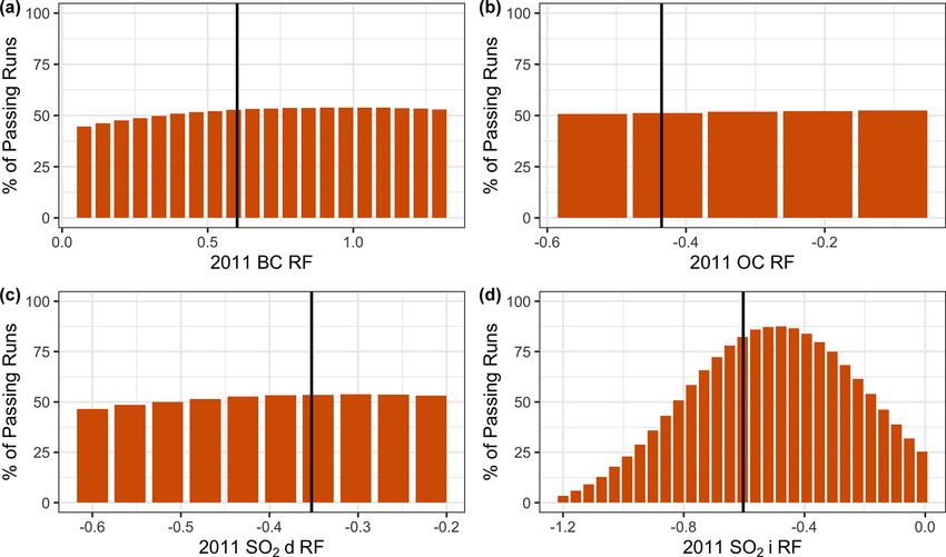
K. Dorheim et al.: HIRM v1.0                                                                                                 367

2013; Van Vuuren 2011; Millar et al., 2015; Boas, 2006).           forcing agent since there are no gas cycle or forcing interac-
By relying on a process-based climate model to compute re-         tions with other species within Hector, making it straightfor-
sponse function (RF) values, HIRM is able to use a linear          ward to derive the IRF, but other forcing agents could have
IRF in a simple impulse response model and capture the ma-         been selected for the perturbation run. During the reference
jor nonlinear dynamics between the emissions to radiative          model run Hector was driven with the Representative Con-
forcing calculations by using radiative forcing time series as     centration Pathway (RCP) 4.5 scenario, while for the pertur-
input data.                                                        bation model run BC emissions were doubled relative to RCP
   HIRM calculates the atmospheric temperature change              4.5 BC emissions in a single year. RCP 4.5 CO2 concentra-
from preindustrial temperature (T ) as the sum of the temper-      tions were prescribed during these runs, suppressing Hector’s
ature contribution from individual forcing agents Ti (Eq. 1):      normal carbon cycle–temperature feedbacks.
           n
                                                                      For the two validation experiments we did not include car-
                                                                   bon cycle–climate feedbacks into the IRF as we wanted to
           X
T (t) =          Ti (t).                                    (1)
           i=1                                                     examine the relative importance of nonlinearities in emission
                                                                   to forcing calculations, at least as represented in Hector, as
Here the individual temperature contribution is equal to the       compared to nonlinearities in Hector’s forcing to tempera-
convolution of the radiative forcing time series RFi with the      ture calculations (as represented within DOECLIM). For this
temperature response to a radiative forcing pulse IRFi for a       reason the IRF should represent only the response of tem-
single radiative forcing agent (Eq. 2).                            perature to radiative forcing; otherwise, the temperature re-
                                                                   sponse from these feedback mechanisms would be incorpo-
           Zt
                                                                   rated into the IRF, which would then be doubled-counted as
Ti (t) =        RFi (t 0 )IRFi (t − t 0 )dt 0               (2)
                                                                   forcing time series are being used as inputs. For the replica-
           t0                                                      tion experiments we also focus on reproducing Hector tem-
The method we used to obtain RFi and IRFi for HIRM re-             perature without carbon–climate feedbacks. Other applica-
lies on output from a parent process-based model. The subse-       tions of HIRM may require IRFs that include the temperature
quent sections discuss how we obtained RFi and IRFi specif-        response from carbon cycle feedbacks.
ically from Hector. It is important to note that while HIRM           The temperature response (Tresponse ) to the BC emissions
can be set up with unique IRFs for each radiative forcing          perturbation is equal to the difference between
                                                                                                                   the reference
agent (as demonstrated below), this was not done in this ap-       (Tref ) and perturbation temperature Tp (Eq. 3), with the per-
plication since Hector uses one IRF for all species.               turbation occurring at year t0 :
   HIRM is an open-source R package (https://github.com/           Tresponse (t − t0 ) = Tp (t − t0 ) − Tref (t − t0 ) .      (3)
jgcri/hirm, last access: 11 January 2021) with Doxygen-style
comments, unit tests, and online documentation via pkgdown         The temperature response to a radiative forcing perturbation
(Wickham and Hesselberth, 2020). The online documenta-             was calculated by dividing the temperature response to the
tion available at https://jgcri.github.io/HIRM/ (last access:      emissions perturbation by the size of the radiative forcing
11 January 2021) documents all of the package functions and        pulse (Eq. 4). The size of the radiative forcing pulse (Xy )
links with a vignette (example) that demonstrates how to set       was set equal to the difference in radiative forcing between
up and run HIRM. The package contains all of the IRFs and          the reference and emissions perturbation runs (described in
RF inputs used in this paper that can be used in a customiz-       the paragraph above) in the perturbation year:
able configuration matrix to set up and run HIRM.
                                                                   IRFi (t − t0 ) = Tresponse (t − t0 ) /Xy .                 (4)
2.3   IRF derivation
                                                                   This IRF had a length of 300 years, in order to ensure the IRF
As previously mentioned, one of Hector’s assumptions is            was long enough to be convolved with the RF inputs; the
that all of Hector’s radiative forcing agents elicit the same      end of the IRF was extrapolated with an exponential decay
temperature response to a change in radiative forcing. Even        function to a length of 3000 years with a decay constant of
though HIRM can use a unique IRF for each radiative forc-          0.20. Extending the length of the IRF prevents the IRF from
ing agent, for the purposes of HIRM validation exercises in        being padded with zeros and having to truncate the RF inputs.
this study, HIRM’s setup must be analogous to that of its par-        The majority of Hector’s temperature response to a radia-
ent model Hector. In this study we configured HIRM with a          tive forcing pulse occurs within the first 50 years after the
single IRF that characterizes Hector’s temperature response        perturbation (Fig. 1). The strongest response occurs during
to all of its 37 radiative forcing agents, derived from a refer-   the perturbation year itself, with a maximum value of 0.09
ence run and a black carbon (BC) emissions perturbation run        (◦ C W−1 m−2 ); by year 35 the temperature response has de-
of Hector. In Hector, BC emissions are converted directly to       creased by 97 % and continues to approach zero for the re-
radiative forcing, and therefore an emissions pulse of BC is       mainder of the IRF. This IRF is used in both of the validation
analogous to a radiative forcing pulse. BC was chosen as the       experiments and case studies except where noted.

https://doi.org/10.5194/gmd-14-365-2021                                                    Geosci. Model Dev., 14, 365–375, 2021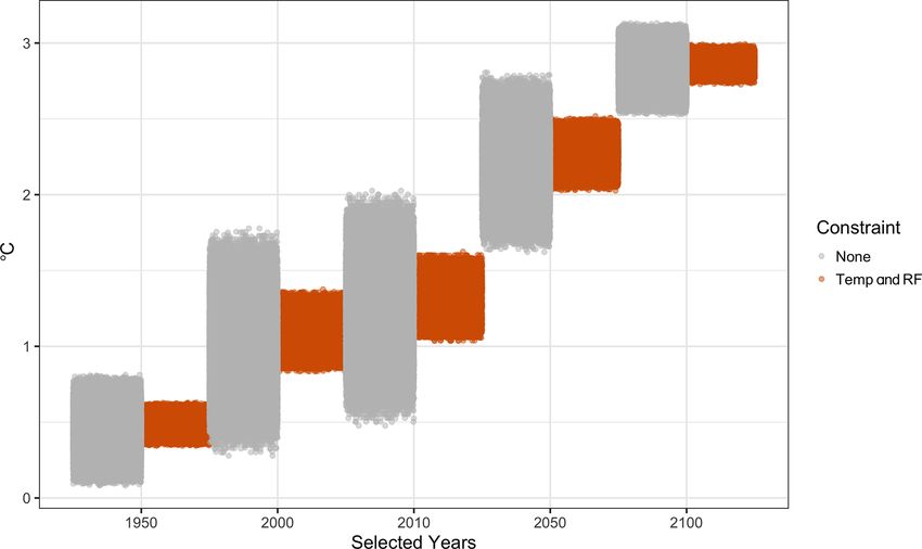
368 K. Dorheim et al.: HIRM v1.0
CO2 concentration step. The abrupt 4 times CO2 concentra-
tion step is a test commonly used by climate modelers to un-
derstand the climate system’s response to CO2 (Taylor et al.,
2012). In this experiment HIRM was set up with the Hector-
derived IRF and a RF input from an abrupt 4 times CO2
concentration step. The radiative forcing time series was ob-
tained from Hector runs following the CMIP5 protocol (Tay-
lor et al., 2012). HIRM’s radiative forcing time series input
was the difference in Hector radiative forcing from Hector
Figure 1. The first 50 years of the global temperature response driven with a constant CO2 concentration of 278 ppm and
to a radiative forcing perturbation for Hector v2.0; the remain- Hector driven with a CO2 concentration of 278 ppm until the
ing 2500 years of the impulse response are almost constant and year 2010 when the CO2 concentration increased by a mag-
slowly approach zero. Here the black carbon emissions were dou-
nitude of 4 and remained constant for the rest of the run. The
bled in 2010 relative to the Representative Concentration Pathway
difference in Hector’s global mean temperature anomaly be-
4.5 value.
tween the constant reference run and the perturbed step run
was then compared with HIRM’s output.
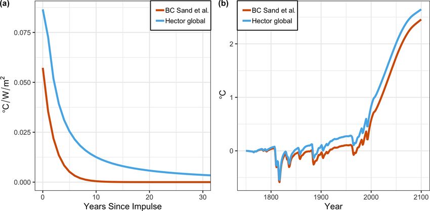
3 Validation experiments HIRM reproduced Hector’s abrupt 4 times CO2 concen-
tration step temperature response with a high degree of accu-
3.1 Replication of RCP results racy (Fig. 2b). The RMSE between HIRM and Hector tem-
perature output from the abrupt CO2 concentration step was
Emulation is used to validate HIRM by illustrating that the 1.5 × 10⁻¹⁹ ◦ C with a cumulative percent difference of 0 %.
HIRM framework reproduces the dynamics of a process- The abrupt CO2 concentration step is a standard diagnostic
based SCM with a minimal loss of information. If HIRM test used to examine climate model responses (Taylor et al.,
can accurately reproduce or emulate the atmospheric temper- 2012; Eyring et al., 2016). Since HIRM was able to accu-
ature of a more complex, process-based model such as Hec- rately emulate Hector’s temperature response to a large step
tor, then we assume that HIRM is able to capture important perturbation, we conclude that the majority of the nonlin-
nonlinear dynamics of the climate system using this setup, at earities within Hector are occurring during the emissions-
least to the extent these are captured in the SCM. Conversely, to-radiative forcing portion of the emissions-to-temperature
if HIRM is unable to reproduce Hector’s global temperature causal chain. While this is to be expected from the general
outputs, this would indicate that important processes are not principles of SCMs, it nonetheless provides a useful check
being captured by the HIRM framework. that our understanding of the parent model’s behavior is cor-
In the first validation experiment, HIRM was set up to re- rect.
produce Hector temperature for RCP 2.6, RCP 4.5, RCP 6.0,
and RCP 8.5. HIRM was configured for each RCP scenario
with a single IRF derived from Hector (Fig. 1) together with a 4 HIRM application case studies
complete set of time series from Hector’s 37 radiative forcing
agents. The radiative forcing time series for these validation 4.1 Aerosol uncertainty case study
experiments came from Hector output from RCP 2.6, 4.5,
6.0, and 8.5 with prescribed CO2 concentrations. The global Uncertainties in the magnitude of historical and future radia-
mean temperature outputs from Hector driven with RCP 2.6, tive forcing effects continue to be a crucial challenge for cli-
RCP 4.5, RCP 6.0, and RCP 8.5 were saved and used as val- mate science research, and this is particularly true for aerosol
idation data for HIRM. effects (Forest, 2018). In this first case study HIRM was used
HIRM was able to emulate Hector’s temperature for the to explore a range of future temperature change when ac-
four RCPs with a minimal loss of information (Fig. 2a). counting for uncertainty in some aerosol radiative forcing ef-
The difference between HIRM and Hector total tempera- fects, specifically black carbon (BC), organic carbon (OC),
ture, measured as the root-mean-squared error (RMSE), was indirect SO2 effects (SO2 i), and direct SO2 effects (SO2 d).
1.3 × 10⁻⁹ ◦ C (Fig. 2a) for each RCP scenario. The cumu- To do so, HIRM was again set up to recreate Hector’s RCP
lative percentage difference between HIRM and Hector tem- 4.5 temperature. In this analysis, BC, OC, SO2 i, and SO2 d
perature was 0 % (rounded from 1.0 × 10⁻⁵ ; other 0 % re- RF inputs were varied. Aerosol cloud indirect effects are rep-
sults are similar) for each RCP scenario. resented in Hector as a function of SO2 emissions only, and
thus we refer to that as SO2 indirect forcing. We present a
3.2 Replication of 4 times CO2 results simple demonstration of the model in this case study and
note that we have not produced probabilistic results but an
The second validation experiment tested HIRM’s ability to illustrative range of temperature pathways that result from
reproduce Hector’s temperature response to an abrupt 4 times aerosol uncertainties (e.g., Smith and Bond, 2014). A full
Geosci. Model Dev., 14, 365–375, 2021 https://doi.org/10.5194/gmd-14-365-2021K. Dorheim et al.: HIRM v1.0 369
Figure 2. Comparison of Hector (dashed gray line) and HIRM (dashed blue line) global mean temperature anomaly from the two validation
experiments. In panel (a) HIRM was used to the recreate Hector temperature for the four RCPs. The four lines in panel (a) from lowest to
highest 2100 temperature represent results for RCP 2.6, RCP 4.5, RCP 6.0, and RCP 8.5. Panel (b) compares the temperature response of
HIRM and Hector from the abrupt 4 times CO2 concentration step validation test.
Table 1. The minimum and maximum 2011 radiative forcing values perature change. The 2011 aerosol (SO2 i, SO2 d, BC, + OC)
from IPCC AR5 8.SM (Table 5 of Myhre et al., 2013). These values radiative forcing was constrained to pass through an uncer-
were used to obtain the min and max aerosol uncertainty scalers for tainty range [−1.66 to 0.14 W m−2 ] (similar to Myhre et al.,
four RF agents (BC, OC, SO2 i, and SO2 d). Along with the 2011 RF 2013, but adjusted to account for nitrate and dust forcing and
of the default configuration of HIRM and Hector for RCP 4.5. empirical constraints; see the discussion in Smith and Bond,
2014). HIRM temperature trend was calculated as the slope
RF Min. 2011 Max. 2011 Hector default of a linear regression and then compared to the observed tem-
agent RF RF 2011 RF
perature trend range of [0.65 to 1.1] ◦ C over 1880–2012 re-
BC 0.05 0.87 0.40 ported by Hartmann et al. (2013). Cases that did not meet
OC −0.21 −0.04 −0.17 these constraints were removed (see Fig. 3).
SO2 i −1.2 0 −0.60 We found that the historical constraints had an unequal im-
SO2 d −0.6 −0.2 −0.35 pact on the scaled radiative forcing impacts. The tempera-
ture at the end of the century for the unconstrained ensem-
ble ranged over 2.5–3.1 ◦ C; incorporating the historical con-
straints into the uncertainty analysis narrowed uncertainty in
probabilistic analysis would also involve varying additional future temperature to 2.7–2.9 ◦ C (Fig. 3). The historical con-
parameters, such as climate sensitivity, ocean heat update, straints had different impacts on the sampled aerosol uncer-
and carbon cycle parameters. tainty scalers. All of the sampled OC scalers passed through
The aerosol uncertainty scalers were generated from the the historical constraints (Fig. 4b), while the constraints had
2011 aerosol radiative forcing ranges reported in IPCC AR5 a modest effect on the OC, BC, and SO2 d scalers (Fig. 4a, b,
8.SM Table 5 (Myhre et al., 2013). The BC, OC, SO2 i, and and c).
SO2 d radiative forcing IPCC ranges were individually sam- The historical constraints have the most noticeable ef-
pled at intervals of 0.04 W m−2 in 2011 (Table 1), resulting fect on the SO2 i uncertainty scalers. This is because of the
in a total of 29 000uncertainty scalar combinations. Default large absolute magnitude of the uncertainty in aerosol indi-
HIRM 2011 BC, OC, SO2 i, and SO2 d radiative forcing val- rect effects (Myhre et al., 2013), which results in a large role
ues were then divided by the values sampled from the respec- for assumptions about the strength of aerosol indirect cool-
tive IPCC ranges to obtain the uncertainty scalers. ing (Tomassini et al., 2007; Meinshausen et al., 2009). This
HIRM was set up to run every possible combination of shows that strong (negative) aerosol indirect forcing is con-
the scaled RF time series a total of 29 000 times. This cre- sistent with only a few numerical combinations of forcing
ated an ensemble of uncertainty runs, whose results were values from other species, at least for default Hector climate
constrained (i.e., filtered) by historical radiative forcing and system parameters. The sample analysis using HIRM illus-
temperature. HIRM total radiative forcing was constrained to trates how this modeling framework can be utilized to calcu-
match IPCC historical estimates in radiative forcing and tem-
https://doi.org/10.5194/gmd-14-365-2021 Geosci. Model Dev., 14, 365–375, 2021370 K. Dorheim et al.: HIRM v1.0 Figure 3. The temperature (◦ C) spread from the aerosol uncertainty runs in selected years. The gray regions show all of the possible runs before the historical constraints were put into the place; orange regions are the runs that passed through both historical temperature and radiative forcing constraints. The uncertainty in temperature due to uncertainty in aerosol forcing decreases by 2100 because emissions of aerosols and precursor compounds decrease over time so their influence on temperature decays over time as well. We note that uncertainty in other climate system parameters, such as climate sensitivity and ocean heat diffusivity, were not samples in this application. Including these uncertainties would alter these results. Note that temperature change in 2020 is larger than the applied historical constraint ([0.65 to 1.1] ◦ C over 1880–2012) because temperatures in this figure are relative to 1750. Figure 4. Uncertainty scalers used to vary (a) black carbon, (b) organic carbon, (c) direct SO2 effects, and (d) indirect SO2 effects aerosol RF time series in the uncertainty analysis. HIRM was run a total of 29 000 times, with every combination of uncertainty scaler represented on the x axes of panels (a)–(d), creating an ensemble of uncertainty runs with scalars varying for all radiative forcing agents. Each panel of this figure plots a projection of the percent of runs passing through the historical constraints as the 2011 radiative forcing agent of an agent is varied. The vertical black line marks default 2011 RF. Geosci. Model Dev., 14, 365–375, 2021 https://doi.org/10.5194/gmd-14-365-2021
K. Dorheim et al.: HIRM v1.0                                                                                                  371

late the range of past and future temperature changes under        133 Tg BC emissions change (used in Sand et al., 2015) using
assumed uncertainty in aerosol radiative forcing.                  Hector’s default forcing per unit BC emission assumptions.
                                                                   With this transformation we have replaced Hectors’ default
4.2   HIRM as a tool for development: case study                   BC representation in HIRM with the Sand et al. (2015) tem-
                                                                   perature response in both magnitude and temporal behavior.
Radiative forcing effects from aerosols are complex (Fan et           We found that the BC Sand et al. (2015) IRF has a weaker
al., 2016; Bond et al., 2013), and while the physics driving       temperature response in the perturbation year and a more
these complexities have been incorporated into ESMs, they          rapid decline in temperature response compared to Hector’s
are not considered in most SCMs. For example, consider             global IRF (Fig. 5a). The maximum IRF response for the BC
black carbon (BC): unlike cooling effects from aerosols that       Sand et al. (2015) IRF is 0.06 (◦ C W−1 m−2 ), which is 0.03
scatter shortwave radiation back into space, BC heats within       (◦ C W−1 m−2 ) cooler than Hector’s IRF. In addition, the BC
the atmosphere and also at the surface when deposited on           Sand et al. (2015) IRF approaches 0 (◦ C W−1 m−2 ) faster
snow or ice, potentially contributing to both cloud indirect       than Hector’s IRF. These differences are expected since the
cooling and heating effects (Bond et al., 2013). It can also in-   BC Sand et al. IRF was derived from the NorESM-1 ESM,
crease cloud amounts, as BC atmospheric heating stabilizes         meaning that this IRF incorporates the complex cooling and
the atmospheric thermal profile (Bond et al., 2013). Experi-       warming effects of BC emissions, the net warming over land
ments conducted with ESMs have found large differences in          as compared to no net warming over oceans (Sand et al.,
the response to a step change in BC emissions compared to a        2015). When HIRM was configured with the BC Sand et
step change in CO2 (Sand et al., 2015; Yang et al., 2019).         al. (2015) IRF, the global temperature was lower by 0.2 ◦ C
   Incorporating these dynamics into Hector would be a non-        from 1750 to 2100 under the RCP 4.5 scenario (Fig. 5b).
trivial task, but HIRM can be used to estimate what effect         Based on these results, if Hector were modified to emulate
they would have on the model’s global temperature. For this        this BC response, we predict that the model’s global temper-
case study, HIRM was set up to emulate Hector RCP 4.5 as           ature would be cooler by approximately 0.2 ◦ C in 2100.
before but with one difference: instead of pairing the BC RCP         We note that the idea of different forcing agents has been
4.5 RF time series with Hector’s single IRF, the BC RCP            around for quite some time. For example, this has been incor-
4.5 RF time series was paired with a BC-specific IRF. Since        porated mechanistically for aerosols in the MAGICC model
HIRM is set up with a BC-specific IRF, the results will no         for around 30 years now (Wigley and Raper, 1992), and
longer be equivalent to Hector’s. Instead, the results illus-      more recently inferred by Shindell (2014) from General Cir-
trate what Hector’s temperature could be if the BC dynamics        culation Model results. Richardson et al. (2019) used sepa-
were modified.                                                     rate response functions for CO2 , CH4 , solar insolation, and
   The BC-specific IRF was derived using output from a             aerosols, although the differences in these response func-
study that performed BC emission step tests with the ESM           tions were not discussed. As further information on species-
NorESM-1 (Sand et al., 2015). Mathematically, the deriva-          specific IRFs become available it will be important to quan-
tive of a step response is equal to the impulse response func-     tify the consequences of these different IRFs using tools such
tion, and therefore we can derive an impulse response func-        as HIRM.
tion from the step response results reported in the Sand et
al. (2015) ESM experiment. The temperature response to a
BC step in ESM experiments is well fitted by a single ex-          5   Discussion and conclusion
ponential approach to a constant response (see Yang et al.,
2019, for details). We fit the Sand et al.(2015) abrupt BC         In this paper we document and test HIRM, a framework that
step response as follows:                                          leverages the nonlinear dynamics of process-based SCMs
                  −t                                               within a computationally efficient, highly idealized linear im-
T (t) = A (1 − e τ ).                                       (5)    pulse response model. Our two case studies demonstrate that
                                                                   HIRM can be used as a test bed to quickly examine the con-
The results of a nonlinear optimization of this function re-       sequences of different model assumptions, and to estimate
turned values of and τ that were 1.8 ◦ C and 2.1 years, respec-    changes in parent model behavior from including new mech-
tively. These optimal values were used in Eq. (6), the differ-     anisms. While other IRF-based models have incorporated
entiated form of Eq. (5), to provide a numerical BC tempera-       nonlinear dynamics using a number of approaches (Hooss et
ture impulse response function corresponding to the Sand et        al., 2001; Millar et al., 2017, ADD), HIRM is able to demon-
al. (2015) result:                                                 strate nonlinear dynamics through its use of exogenous forc-
           A −y                                                    ing inputs from Hector. HIRM is available as an open-source
Rt (t) =     e t dt.                                        (6)    R package (available at https://github.com/JGCRI/HIRM,
           τ
                                                                   last access: 11 January 2021), its computational flexibility
The numerical result of Eq. (6) is converted to a BC impulse       and short run time make it particularly appropriate for uncer-
response per unit forcing by dividing by the forcing from a        tainty analyses and experimental SCM design.

https://doi.org/10.5194/gmd-14-365-2021                                                Geosci. Model Dev., 14, 365–375, 2021
372 K. Dorheim et al.: HIRM v1.0 Figure 5. (a) Hector’s IRF (blue) compared with the BC Sand et al. (2015) IRF (red). (b) HIRM total temperature for the Representative Concentration Pathway 4.5 for two HIRM cases: one that only uses Hector’s IRF (blue) and the other pairing the BC RF time series with the BC Sand et al. (2015) IRF (red). We demonstrated that HIRM can be used to examine ing from forcing to temperature. If this finding holds for a uncertainty within the climate system, and that incorporat- wider class of models, this would mean that a wide range of ing a more realistic BC temperature response into Hector model responses to forcing could be quickly simulated using has a significant impact on Hector’s global temperature. If IRFs. Good et al. (2013) showed that SCMs based on step more studies corroborate the findings of Sand et al. (2015) responses work fairly well for reproducing General Circula- and Yang et al. (2019) by observing shorter timescale re- tion Model (GCM) results, suggesting that the assumptions sponses for BC temperature dynamics across a number of underlying HIRM are valid. ESMs and Atmosphere–Ocean General Circulation Models The case studies showcase HIRM’s flexibility, which is (AOGCMs), then SCM modeling groups will need to con- based on HIRM’s dependence on a parent model. Arguably sider incorporating the BC temperature response dynamics this can be viewed as a limitation or a tradeoff and allows into SCMs. Some SCMs, such as MAGICC 5.3 and MAG- HIRM to be used as a tool for rapid exploration. One lim- ICC 6 (Tang and Riley, 2015), already exhibit multiple tem- itation of this framework is that interactions between forc- perature responses; interestingly, MAGICC has a shorter ing agents are not directly considered. For example, multiple timescale for the temperature response for aerosols (Schwar- species of aerosols may contribute to cloud-indirect cooling ber et al., 2019), but the resulting response in MAGICC still effects. These interactions, however, are not well constrained has a longer timescale than that from the AOGCMs (Sand et (Fan et al., 2016), and for many purposes where SCMs might al., 2015; Yang et al., 2019). be applicable, it is most important to be able to represent During the HIRM validation experiments we demonstrate the overall (large) uncertainty range, rather than interactions that most of nonlinearities are in the emissions to forc- among species that have yet to be definitively quantified. An ing steps, in which the SCM calculates concentrations from effort to represent aerosol indirect effects semi-analytically emissions and radiative forcings from concentrations, rela- (Ghan et al., 2013) demonstrated not only the multiple pro- tionships that are widely used (Etminan et al., 2016). In com- cesses that are relevant but also the difficulty in understand- parison the nonlinearities in going from forcing to global ing the drivers of the different forcing estimates from more mean temperature are relatively minor. This implies that ef- complex models. forts to improve the representation of nonlinear behavior in Insights gained from HIRM could be useful in future work SCMs should be focused on emissions-to-forcing processes. applying impulse response functions in general and the de- We note that we draw this conclusion by calibrating HIRM to sign of simple climate models in particular. We suggest that a single process-based SCM; this finding should be verified improvements to simple climate models should focus on im- using other models, including Earth System Models of In- proving the representation of emission-to-concentration and termediate Complexity (Claussen et al., 2002). Such EMICs concentration-to-forcing relationships. As we note above, have more physically based parameterizations but low lev- however, it would be useful to also design comparisons with els of internal model noise, which would be valuable for more complex models, perhaps EMICs given their lower exploring the magnitude and nature of nonlinearities in go- noise and computational requirements, to determine the ex- Geosci. Model Dev., 14, 365–375, 2021 https://doi.org/10.5194/gmd-14-365-2021
K. Dorheim et al.: HIRM v1.0                                                                                                       373

tent to which the temperature response to forcing in more           Bond-Lamberty, 2020). Code and results related to the dis-
complex models can be accurately represented by impulse             cussion and conclusions of this paper are available on the
response functions, particularly on 20–30 year timescales           Open Science Framework (OSF) at https://osf.io/kmrj8/ and
where GCM outputs are particularly noisy.                           https://doi.org/10.17605/OSF.IO/KMRJ8 (Dorheim et al., 2020b).
   HIRM could also be used with data generated by other
SCMs. This could be a useful way of decomposing differ-
ences in responses between SCMs (e.g., Nicholls et al., 2020)       Author contributions. SJS conceptualized the Hybrid Impulse Re-
                                                                    sponse Model (HIRM). KD and BBL developed the project soft-
into differences in the emissions to forcing step compared
                                                                    ware. KD wrote the manuscript with contributions from all co-
to differences in the model’s response to a forcing impulse.
                                                                    authors.
Similarly, HIRM could be used to examine the uncertainty
due to the different forcing to temperature responses amongst
SCMs (see Schwarber et al., 2019, for examples of different         Competing interests. The authors declare that they have no conflict
forcing to temperature IRFs).                                       of interest.
   HIRM can be used as a test bed for future SCM devel-
opment. As demonstrated here, the incorporation of a GCM-
derived temperature response function for black carbon emis-        Acknowledgements. We thank Robert Link for invaluable insight
sions results in a significantly different global mean temper-      regarding HIRM development as an R package and Maria Sand for
ature response (Fig. 5). Exploration of the potential impact        numerical model results. This research was supported by the United
of such changes can be done quickly in HIRM to decide               States Environmental Protection Agency.
if changes should be incorporated into, for example, Hec-
tor. Incorporating such a change into the Hector model itself
would be a more time- and labor-intensive process for sev-          Financial support. Research contributions were supported by the
eral reasons. First, to incorporate this change into Hector one     U.S. Environmental Protection Agency, Climate Change Divi-
would need to decide how to physically interpret the faster         sion, under Interagency Agreements (nos. DW8992395101 and
                                                                    DW08992459801).
BC response time seen in GCMs since Hector does not use
impulse response functions directly. There is some debate
whether this is due to different response over land vs. ocean
                                                                    Review statement. This paper was edited by Juan Antonio Añel and
or if this is more closely related to differing hemispheric re-
                                                                    reviewed by Kuno Strassmann and two anonymous referees.
sponses (Meinshausen et al., 2011; Shindell, 2014; Sand et
al., 2015). Further, explorations or model extensions using
HIRM can be accomplished without a user having to under-
stand Hector’s code, dependencies, and coding standards.
   Finally, this framework could also be used for analysis          References
that requires capabilities not present in SCMs, for exam-
ple, regional analysis. Regional temperature trends could be        Acosta Navarro, J. C., Varma, V., Riipinen, I., Seland, Ø.,
simulated by HIRM by incorporating the ratio of regional              Kirkevåg, A., Struthers, H., Iversen, T., Hansson, H.-C., and
to global temperature responses for each forcing agent into           Ekman, A. M. L.: Amplification of Arctic warming by past
                                                                      air pollution reductions in Europe, Nat. Geosci., 9, 277–281,
HIRM (Sand et al., 2019; Shindell et al., 2009). This could
                                                                      https://doi.org/10.1038/ngeo2673, 2016.
be particularly valuable for a region such as the Arctic, where
                                                                    Boas, M. L.: Mathematical Methods in the Physical Sci-
a variety of forcing agents, such as regional sulfate (Acosta         ences, Wiley, available at: https://books.google.com/books?id=
Navarro et al., 2016) and local black carbon (Sand et al.,            1xV0CgAAQBAJ (last access: 11 January 2021), 2006.
2015; Yang et al., 2019), and global forcing changes, e.g.,         Bond, T. C., Doherty, S. J., Fahey, D. W., Forster, P. M., Berntsen,
Arctic amplification, all may play a role. This type of anal-         T., DeAngelo, B. J., Flanner, M. G., Ghan, S., Kärcher, B., Koch,
ysis could be readily accomplished using HIRM, including              D., Kinne, S., Kondo, Y., Quinn, P. K., Sarofim, M. C., Schultz,
the wide range of uncertainty space that should be examined           M. G., Schulz, M., Venkataraman, C., Zhang, H., Zhang, S.,
(e.g., Fig. 3). Future research with HIRM could test IRFs set         Bellouin, N., Guttikunda, S. K., Hopke, P. K., Jacobson, M.
up with different climate sensitivity values and inputs from          Z., Kaiser, J. W., Klimont, Z., Lohmann, U., Schwarz, J. P.,
other process-based models.                                           Shindell, D., Storelvmo, T., Warren, S. G., and Zender, C. S.:
                                                                      Bounding the role of black carbon in the climate system: A sci-
                                                                      entific assessment, J. Geophys. Res.-Atmos., 118, 5380–5552,
                                                                      https://doi.org/10.1002/jgrd.50171, 2013.
Code availability. The HIRM R package is available at https:
                                                                    Claussen, M., Mysak, L., Weaver, A., Crucifix, M., Fichefet, T.,
//github.com/JGCRI/HIRM (last access: 11 January 2021) with
                                                                      Loutre, M.-F., Weber, S., Alcamo, J., Alexeev, V., Berger, A.,
an online manual available at https://jgcri.github.io/HIRM/ (last
                                                                      Calov, R., Ganopolski, A., Goosse, H., Lohmann, G., Lunkeit,
access: 11 January 2021). The package is also archived on
                                                                      F., Mokhov, I., Petoukhov, V., Stone, P., and Wang, Z.: Earth sys-
Zenodo (https://doi.org/10.5281/zenodo.3756122, Dorheim and
                                                                      tem models of intermediate complexity: closing the gap in the

https://doi.org/10.5194/gmd-14-365-2021                                                   Geosci. Model Dev., 14, 365–375, 2021
374 K. Dorheim et al.: HIRM v1.0
spectrum of climate system models, Clim. Dynam., 18, 579–586, Second Assessment Report: IPCC Technical Paper 2, Tech. rep.,
https://doi.org/10.1007/s00382-001-0200-1, 2002. Intergovernmental Panel on Climate Change, 1997.
Dorheim, K. and Bond-Lamberty, B.: JGCRI/HIRM: Dorheim Hurrell, J. W., Holland, M. M., Gent, P. R., Ghan, S., Kay, J. E.,
et al. 2020 submitted to GMD (Version v1.0.0), Zenodo, Kushner, P. J., Lamarque, J.-F., Large, W. G., Lawrence, D.,
https://doi.org/10.5281/zenodo.3756122, 2020. Lindsay, K., Lipscomb, W. H., Long, M. C., Mahowald, N.,
Dorheim, K., Link, R., Hartin, C., Kravitz, B., and Snyder, A.: Cal- Marsh, D. R., Neale, R. B., Rasch, P., Vavrus, S., Vertenstein,
ibrating simple climate models to individual Earth system mod- M., Bader, D., Collins, W. D., Hack, J. J., Kiehl, J., and Mar-
els: Lessons learned from calibrating Hector, Earth Space Sci., 7, shall, S.: The Community Earth System Model: A Framework
https://doi.org/10.1029/2019EA000980, 2020a. for Collaborative Research, B. Am. Meteorol. Soc., 94, 1339–
Dorheim, K. R., Smith, S. J., and Bond-Lamberty, B.: 1360, https://doi.org/10.1175/BAMS-D-12-00121.1, 2013.
Code and Data for A hybrid impulse response model Joos, F. and Bruno, M.: Pulse response functions are cost-efficient
for climate modeling and uncertainty analyses, OSF, tools to model the link between carbon emissions, atmospheric
https://doi.org/10.17605/OSF.IO/KMRJ8, 2020b. CO2 and global warming, Phys. Chem. Earth, 21, 471–476,
Etminan, M., Myhre, G., Highwood, E. J., and Shine, K. P.: Radia- https://doi.org/10.1016/S0079-1946(97)81144-5, 1996.
tive forcing of carbon dioxide, methane, and nitrous oxide: A sig- Joos, F., Müller-Fürstenberger, G., and Stephan, G.: Correcting the
nificant revision of the methane radiative forcing, Geophys. Res. carbon cycle representation: How important is it for the eco-
Lett., 43, 12614–12623, https://doi.org/10.1002/2016GL071930, nomics of climate change?, Environ. Model. Assess., 4, 133–140,
2016. https://doi.org/10.1023/A:1019004015342, 1999.
Eyring, V., Bony, S., Meehl, G. A., Senior, C. A., Stevens, B., Joos, F., Roth, R., Fuglestvedt, J. S., Peters, G. P., Enting, I. G.,
Stouffer, R. J., and Taylor, K. E.: Overview of the Coupled von Bloh, W., Brovkin, V., Burke, E. J., Eby, M., Edwards, N.
Model Intercomparison Project Phase 6 (CMIP6) experimen- R., Friedrich, T., Frölicher, T. L., Halloran, P. R., Holden, P.
tal design and organization, Geosci. Model Dev., 9, 1937–1958, B., Jones, C., Kleinen, T., Mackenzie, F. T., Matsumoto, K.,
https://doi.org/10.5194/gmd-9-1937-2016, 2016. Meinshausen, M., Plattner, G.-K., Reisinger, A., Segschneider,
Fan, J., Wang, Y., Rosenfeld, D., and Liu, X.: Review of Aerosol– J., Shaffer, G., Steinacher, M., Strassmann, K., Tanaka, K., Tim-
Cloud Interactions: Mechanisms, Significance, and Challenges, mermann, A., and Weaver, A. J.: Carbon dioxide and climate im-
J. Atmos. Sci., 73, 4221–4252, https://doi.org/10.1175/JAS-D- pulse response functions for the computation of greenhouse gas
16-0037.1, 2016. metrics: a multi-model analysis, Atmos. Chem. Phys., 13, 2793–
Forest, C. E.: Inferred Net Aerosol Forcing Based on Historical Cli- 2825, https://doi.org/10.5194/acp-13-2793-2013, 2013.
mate Changes: a Review, Current Climate Change Reports, 4, Kriegler, E.: Imprecise probability analysis for integrated assess-
11–22, https://doi.org/10.1007/s40641-018-0085-2, 2018. ment of climate change, dissertation, 2005.
Ghan, S. J., Smith, S. J., Wang, M., Zhang, K., Pringle, K., Carslaw, Link, R., Bond-Lamberty, B., Hartin, C., Shiklomanov, A., bveg-
K., Pierce, J., Bauer, S., and Adams, P.: A simple model of global awe, Patel, P., Willner, S., Dorheim, K. R., Gieseke, R., Smith,
aerosol indirect effects, J. Geophys. Res.-Atmos., 118, 6688– S., and Lynch, C.: JGCRI/hector: Hector version 2.3.0, Zenodo,
6707, https://doi.org/10.1002/jgrd.50567, 2013. https://doi.org/10.5281/zenodo.3144007, 2019.
Good, P., Gregory, J. M., Lowe, J. A. and Andrews, T.: Abrupt CO2 Meehl, G. A., Stocker, T. A., Collins, W. D., Friedlingstein, P.,
experiments as tools for predicting and understanding CMIP5 Gregory, J. M., Kitoh, A., Knutti, R., Murphy, J. M., Noda, A.,
representative concentration pathway projections, Clim. Dy- Raper, S. C. B., Watterson, I. G., Weaver, A. J., and Zhao, Z. C.:
nam., 40, 1041–1053, https://doi.org/10.1007/s00382-012-1410- Global Climate Projections, in Climate Change 2007: The Physi-
4, 2013. cal Science Basis, Contribution of Working Group I to the Fourth
Hartin, C. A., Patel, P., Schwarber, A., Link, R. P., and Bond- Assessment Report of the Intergovernmental Panel on Climate
Lamberty, B. P.: A simple object-oriented and open-source Change, Cambridge University Press, Cambridge, United King-
model for scientific and policy analyses of the global cli- dom and New York, NY, USA, 2007.
mate system – Hector v1.0, Geosci. Model Dev., 8, 939–955, Meinshausen, M., Meinshausen, N., Hare, W., Raper,
https://doi.org/10.5194/gmd-8-939-2015, 2015. S. C. B., Frieler, K., Knutti, R., Frame, D. J., and
Hartmann, D. L., Klein Tank, A. M. G., Rusticucci, M., Alexan- Allen, M. R.: Greenhouse-gas emission targets for lim-
der, L. V., Brönnimann, S., Charabi, Y. A. R., Dentener, F. iting global warming to 2 ◦ C, Nature, 458, 1158–1162,
J., Dlugokencky, E. J., Easterling, D. R., Kaplan, A., So- https://doi.org/10.1038/nature08017, 2009.
den, B. J., Thorne, P. W., Wild, M., and Zhai, P.: Observa- Meinshausen, M., Raper, S. C. B., and Wigley, T. M. L.: Em-
tions: Atmosphere and surface, in: Climate Change 2013 the ulating coupled atmosphere-ocean and carbon cycle models
Physical Science Basis, Cambridge University Press, 159–254, with a simpler model, MAGICC6 – Part 1: Model descrip-
https://doi.org/10.1017/CBO9781107415324.008, 2013. tion and calibration, Atmos. Chem. Phys., 11, 1417–1456,
Hooss, G., Voss, R., Hasselmann, K., Maier-Reimer, E., and Joos, https://doi.org/10.5194/acp-11-1417-2011, 2011.
F.: A nonlinear impulse response model of the coupled car- Millar, R. J., Otto, A., Forster, P. M., Lowe, J. A., Ingram, W. J.,
bon cycle-climate system (NICCS), Clim. Dynam., 18, 189–202, and Allen, M. R.: Model structure in observational constraints
https://doi.org/10.1007/s003820100170, 2001. on transient climate response, Climatic Change, 131, 199–211,
Harvey, L. D. D., Gregory, J. M., Hoffert, M., Jain, A., Lal, M., https://doi.org/10.1007/s10584-015-1384-4, 2015.
Leemans, R., Raper, S. C. B., Wigley, T. M. L., and de Wolde, Millar, R. J., Nicholls, Z. R., Friedlingstein, P., and Allen, M. R.:
J.: An Introduction to Simple Climate Models used in the IPCC A modified impulse-response representation of the global near-
surface air temperature and atmospheric concentration response
Geosci. Model Dev., 14, 365–375, 2021 https://doi.org/10.5194/gmd-14-365-2021K. Dorheim et al.: HIRM v1.0 375 to carbon dioxide emissions, Atmos. Chem. Phys., 17, 7213– Stainforth, D. A., Aina, T., Christensen, C., Collins, M., Faull, N., 7228, https://doi.org/10.5194/acp-17-7213-2017, 2017. Frame, D. J., Kettleborough, J. A., Knight, S., Martin, A., Mur- Myhre, G., Shindell, D., Breon, F. M., Collins, W., Fuglestvedt, J., phy, J. M., Piani, C., Sexton, D., Smith, L. A., Spicer, R. A., and Huang, J.: Anthropogenic and Natural Radiative Forcing, in Thorpe, A. J., and Allen, M. R.: Uncertainty in predictions of Climate Change 2013: The Physical Science Basis, Contribution the climate response to rising levels of greenhouse gases, Nature, of Working Group I to the Fifth Assessment Report of the Inter- 433, 403–406, https://doi.org/10.1038/nature03301, 2005. governmental Panel on Climate Change, Cambridge University Stocker, T.: Model Hierarchy and Simplified Climate Models, Press, 2013. in: Introduction to Climate Modelling, Advances in Geophys- Nicholls, Z. R. J., Meinshausen, M., Lewis, J., Gieseke, R., Dom- ical and Environmental Mechanics and Mathematics, Springer, menget, D., Dorheim, K., Fan, C.-S., Fuglestvedt, J. S., Gasser, Berlin, 25–51, 2011. T., Golüke, U., Goodwin, P., Hartin, C., Hope, A. P., Kriegler, Strassmann, K. M. and Joos, F.: The Bern Simple Climate E., Leach, N. J., Marchegiani, D., McBride, L. A., Quilcaille, Y., Model (BernSCM) v1.0: an extensible and fully documented Rogelj, J., Salawitch, R. J., Samset, B. H., Sandstad, M., Shiklo- open-source re-implementation of the Bern reduced-form manov, A. N., Skeie, R. B., Smith, C. J., Smith, S., Tanaka, K., model for global carbon cycle–climate simulations, Geosci. Tsutsui, J., and Xie, Z.: Reduced Complexity Model Intercom- Model Dev., 11, 1887–1908, https://doi.org/10.5194/gmd-11- parison Project Phase 1: introduction and evaluation of global- 1887-2018, 2018. mean temperature response, Geosci. Model Dev., 13, 5175–5190, Tang, J. and Riley, W. J.: Weaker soil carbon–climate feedbacks https://doi.org/10.5194/gmd-13-5175-2020, 2020. resulting from microbial and abiotic interactions, Nat. Clim. Richardson, T. B., Forster, P. M., Smith, C. J., Maycock, A. C., Change, 5, 56–60, https://doi.org/10.1038/nclimate2438, 2015. Wood, T., Andrews, T., Boucher, O., Faluvegi, G., Fläschner, D., Taylor, K. E., Stouffer, R. J., and Meehl, G. A.: An Overview of Hodnebrog, Ø., Kasoar, M., Kirkevåg, A., Lamarque, J.-F., Mül- CMIP5 and the Experiment Design, B. Am. Meteorol. Soc., 93, menstädt, J., Myhre, G., Olivié, D., Portmann, R. W., Samset, 485–498, https://doi.org/10.1175/bams-d-11-00094.1, 2012. B. H., Shawki, D., Shindell, D., Stier, P., Takemura, T., Voulgar- Tomassini, L., Reichert, P., Knutti, R., Stocker, T. F., and Borsuk, akis, A., and Watson-Parris, D.: Efficacy of Climate Forcings in M. E.: Robust Bayesian Uncertainty Analysis of Climate System PDRMIP Models, J. Geophys. Res.-Atmos., 124, 12824–12844, Properties Using Markov Chain Monte Carlo Methods, J. Cli- https://doi.org/10.1029/2019JD030581, 2019. mate, 20, 1239–1254, https://doi.org/10.1175/JCLI4064.1, 2007. Sand, M., Iversen, T., Bohlinger, P., Kirkevåg, A., Seierstad, I., Urban, N. M., Holden, P. B., Edwards, N. R., Sriver, R. Seland, Ø., and Sorteberg, A.: A Standardized Global Climate L., and Keller, K.: Historical and future learning about Model Study Showing Unique Properties for the Climate Re- climate sensitivity, Geophys. Res. Lett., 41, 2543–2552, sponse to Black Carbon Aerosols, J. Climate, 28, 2512–2526, https://doi.org/10.1002/2014GL059484, 2014. https://doi.org/10.1175/JCLI-D-14-00050.1, 2015. van Vuuren, D., Lowe, J., Stehfest, E., Gohar, L., Hof, A., Hope, Schwarber, A. K., Smith, S. J., Hartin, C. A., Vega-Westhoff, B. C., Warren, R., Meinshausen, M., and Plattner, G.-K.: How A., and Sriver, R.: Evaluating climate emulation: fundamental well do integrated assessment models imulate cliamte change?, impulse testing of simple climate models, Earth Syst. Dynam., Climatic Change, 104, 255–285, https://doi.org/10.1007/s10584- 10, 729–739, https://doi.org/10.5194/esd-10-729-2019, 2019. 009-9764-2, 2011. Shindell, D. T.: Inhomogeneous forcing and transient Webster, M., Sokolov, A. P., Reilly, J. M., Forest, C. E., Paltsev, S., climate sensitivity, Nat. Clim. Change, 4, 274–277, Schlosser, A., Wang, C., Kicklighter, D., Sarofim, M., Melillo, https://doi.org/10.1038/nclimate2136, 2014. J., Prinn, R. G., and Jacoby, H. D.: Analysis of climate pol- Shine, K. P., Derwent, R. G., Wuebbles, D. J. and Morcrette, J. J.: icy targets under uncertainty, Climatic Change, 112, 569–583, Radiative forcing of climate, in: Climate Change: The IPCC Sci- https://doi.org/10.1007/s10584-011-0260-0, 2012. entific Assessment, edited by: Houghton, J. T., Jenkins, G. J., and Wenzel, S., Cox, P. M., Eyring, V., and Friedlingstein, P.: Emer- Ephraums, J. J., Cambridge University Press, Cambridge, UK, gent constraints on climate-carbon cycle feedbacks in the CMIP5 41–68, 1990. Earth system models, J. Geophys. Res.-Biogeo., 119, 794–807, Smith, C. J., Forster, P. M., Allen, M., Leach, N., Mil- https://doi.org/10.1002/2013JG002591, 2014. lar, R. J., Passerello, G. A., and Regayre, L. A.: FAIR Wickham, H. and Hesselberth, J.: pkgdown: Make Static HTML v1.3: a simple emissions-based impulse response and car- Documentation for a Package, 2020. bon cycle model, Geosci. Model Dev., 11, 2273–2297, Wigley, T. M. L. and Raper, S. C. B.: Implications for climate and https://doi.org/10.5194/gmd-11-2273-2018, 2018a. sea level of revised IPCC emissions scenarios, Nature, 357, 293– Smith, C. J., Kramer, R. J., Myhre, G., Forster, P. M., Soden, 300, https://doi.org/10.1038/357293a0, 1992. B. J., Andrews, T., Boucher, O., Faluvegi, G., Fläschner, D., Wigley, T. M. L., Smith, S. J., and Prather, M. J.: Radiative Forcing Hodnebrog, Ø., Kasoar, M., Kharin, V., Kirkevåg, A., Lamar- due to Reactive Gas Emissions, J. Climate, 15, 2690–2696, 2002. que, J.-F., Mülmenstädt, J., Olivié, D., Richardson, T., Samset, Yang, Y., Smith, S. J., Wang, H., Mills, C. M., and Rasch, P. J.: B. H., Shindell, D., Stier, P., Takemura, T., Voulgarakis, A., Variability, timescales, and nonlinearity in climate responses to and Watson-Parris, D.: Understanding Rapid Adjustments to Di- black carbon emissions, Atmos. Chem. Phys., 19, 2405–2420, verse Forcing Agents, Geophys. Res. Lett., 45, 12023–12031, https://doi.org/10.5194/acp-19-2405-2019, 2019. https://doi.org/10.1029/2018GL079826, 2018b. Smith, S. J. and Bond, T. C.: Two hundred fifty years of aerosols and climate: the end of the age of aerosols, Atmos. Chem. Phys., 14, 537–549, https://doi.org/10.5194/acp-14-537-2014, 2014. https://doi.org/10.5194/gmd-14-365-2021 Geosci. Model Dev., 14, 365–375, 2021
You can also read