An Integrated Assessment Model of Economy-Energy-Climate - The Model Wiagem
←
→
Page content transcription
If your browser does not render page correctly, please read the page content below
Integrated Assessment                                                                                   1389-5176/02/0304-281$16.00
        2002, Vol. 3, No. 4, pp. 281–298                                                                               # Swets & Zeitlinger

                                        An Integrated Assessment Model
                        of Economy-Energy-Climate – The Model Wiagem

                                                          CLAUDIA KEMFERT

                                     Department of Economics, University of Oldenburg, Oldenburg, Germany

                                                                ABSTRACT

   This paper presents an integrated economy-energy-climate model WIAGEM (World Integrated Assessment General Equilibrium
   Model) incorporating economic, energy and climatic modules in an integrated assessment approach. To evaluate market and non-
   market costs and benefits of climate change, WIAGEM combines an economic approach with a special focus on the international
   energy market, and integrates climate interrelations with temperature changes and sea level variations. WIAGEM is based on 25
   world regions aggregated to 11 trading regions, each with 14 sectors. The representation of the economic relations is based on an
   intertemporal general equilibrium approach and contains the international markets for oil, coal and gas. The model incorporates all
   greenhouse gases (GHG) influencing potential global temperature, sea level variation and the assessed probable impacts in terms of
   climate change costs and benefits. Market and non-market damages are evaluated according to the impact assessment approaches of
   Tol [1]. Additionally, this model includes net changes in GHG-source emissions as well as removals by sinks resulting from land use
   change and de-foresting activities. This paper describes the model structure in detail and outlines general results with emphasis on
   the impacts of climate change. As a result, climate change impacts are significant within the next 50 years; developing regions face
   high economic losses in terms of welfare and GDP losses resulting from sinks and other GHG changes.

Keywords: integrated assessment modeling, Kyoto mechanisms.

1. INTRODUCTION                                                           winter mortality and reduced energy demand for space
                                                                          heating due to higher winter temperatures [2]. Additionally,
Nearly all scientific reports, including the youngest IPCC                working group I of the IPCC reports that the global average
report, confirm once more that humankind’s impact on the                  surface temperature has risen by 0.6  0.2  C over the 20th
natural environment has never been greater and is causing                 century, stressing the fact that the temperature increases in
substantial long-term and irreversible climatic changes. One              the Northern Hemisphere have been the largest of any
important source of climate change are anthropogenic                      century during the past 1,000 years. 1990 was the warmest
greenhouse gas emissions. Increasing atmospheric concen-                  decade and 1998 the warmest year, and the atmospheric
trations of greenhouse gases have a substantial impact on the             concentration of the greenhouse gases carbon dioxide (CO2),
global temperature and sea level which generate extensive                 methane (CH4) and nitrous oxide (N2O) have increased
economic, ecological and climatic impacts. Potential climate              drastically since 1750.
change impacts encompass a general reduction in crop yields                  A comprehensive analysis of all previously described
in most tropical and sub-tropical regions, decreased water                effects caused by climate change must be based on a broad
availability in water-scarce regions, an increased number of              and integrated evaluation tool combining economic, energy
people exposed to vector and water-borne diseases and heat                and climate relations into one modeling instrument, thus al-
stress, intensification in the risk of flooding from heavy                lowing an integrated assessment of the costs and benefits of
precipitation events and rising sea levels, and augmented                 emissions reduction policies. Models based only on eco-
energy demand for space cooling due to higher summer                      nomic, ecological or climate considerations allow an
temperatures. Beneficial impacts include an increased                     assessment of only one aspect of climate change and are
potential crop yield in some higher latitude regions, a                   therefore not comprehensive. Current models trying to inte-
potential increase in global timber supply from appropriately             grate climate interrelations into an economic framework typ-
managed forests, increased water availability, reduced                    ically use stylized and reduced interrelations of all domains.

Address correspondence to: Claudia Kemfert, Department of Economics, University of Oldenburg, D-26111 Oldenburg, Germany. Tel.: þ49 441 798 4106.
Fax: þ49 441 798 4101. E-mail: kemfert@uni-oldenburg.de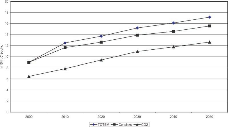
282                                                  CLAUDIA KEMFERT

   This paper presents a novel integrated assessment            modeling approaches covering long-term dynamic effects
modeling approach based on a detailed account of economic       with an intertemporal optimization framework neglect these
relations. Its core is an intertemporal general equilibrium     interregional and intersectoral trade options. We have chosen
model WIAGEM which includes all world regions and main          this economic general equilibrium approach because we
economic sectors. The general equilibrium model also            would like to focus on international trade options and assess
includes a representation of the international energy markets   regional and sectoral effects of different emissions reduction
for oil, coal and gas. The economic model is paired with a      policies. This is due to the fact that most cost benefit climate
model of the ocean carbon cycle and climate.                    change analyses are based on a highly aggregated economic
   WIAGEM comprises a model of 25 world regions                 approach that does not cover sectoral and trade effects.1
aggregated into 11 trading regions, each with 14 sectors.       Because we are applying a detailed representation of the
The model incorporates the greenhouse gases (GHG) CO2,          economy by a CGE approach, we are able on the one hand to
CH4 and N2O, affecting global temperature and sea level;        reproduce detailed regional and sectoral impacts and on the
both determine the impacts of climate change. Market and        other hand only cover (from the climatic perspective) a
non-market impacts are evaluated according to the damage        relatively short time horizon of 50 years.
cost approaches of [3]. Additionally, this model includes net      Costs and benefits of climate change are predominantly
changes in GHG emissions from sources and removals by           assessed by integrated assessment models (IAM) incorpor-
sinks resulting from land use change and de-forestation         ating physical relations of climate change and economic
activities.                                                     effects of damage functions. Integrated assessment models
   The first part of this paper gives a brief overview of       are characterized by combining multidisciplinary ap-
existing economic, climate and ecosystem models and             proaches to thoroughly evaluate climate change impacts.
integrated assessment approaches. The main focus of this        However, as previously described, the economic system is
paper is describing the integrated assessment model             based on a highly aggregated intertemporal optimization
WIAGEM. The model’s economic, energy and climate                framework that neither covers detailed regional and sectoral
modules are thoroughly explained. The paper concludes           interrelations, nor involves international trade effects.
with a short illustration of selected key model results.        Examples for such IAM approaches are MERGE [19],
                                                                RICE or DICE [20], CETA [21] or FUND [22]. Edmonds
                                                                [23] gives an overview of the latest modeling approaches;
2. INTEGRATED ASSESSMENT MODELS                                 previous overviews can be found in Dowlatabadi [24–26].

2.1. Basic Remarks                                              2.2. The Role of Uncertainty
Economic assessment of climate change is based either on
pure economic models focusing on economic relations and         Uncertainty about the future climate is the dominant cause of
interlinkages, economic models enlarged by stylized cli-        uncertainty about the character and significance of impacts.
matic interrelations, or submodels, usually known as            Integrated assessment models cover different uncertainties
integrated assessment (IAM) models. Ecological effects          resulting from data inconsistencies and gaps, unknown
such as the impact of climate change on biodiversity are        functional relationships or errors in the structure of a model,
mainly modeled by ecosystem models concentrating on             and unknown or incorrect assumptions about important
ecological interrelations (see [4–10]). Climatic impacts can    parameter values. Uncertainty about the correct determina-
be assessed chiefly by sophisticated climate models [11–18].    tion of the model, data and key parameter distorts the
   Pure economic models based primarily on an intertem-         understanding of the social, economic and ecologic impacts
poral optimization approach covering aggregated world           of climate change. Uncertainties could justify the postpone-
regions do not normally incorporate a sectoral disaggrega-      ment of significant mitigation efforts. However, uncertainty
tion. In order to assess the impact of climate and ecosystem    also includes the risk of significant climate changes inducing
changes, an integrated assessment model must cover both         considerable impacts. Because the climate change issue is a
climatic and ecosystem as well as economic interrelations.      long-term, global, non-linear and therefore very complex
Economic models including sectoral disaggregation of world      issue, climatic, ecological and economic uncertainties [27]
regions by a general equilibrium model mainly do not            become evident. Economic impacts assessment of climate
embrace ecological or climatic interrelations. In economic      change is based on uncertainties resulting from the above
modeling approaches, there is a trade off between either a      described ecological and climatic uncertainties. Uncertain-
representation and replication of a long term, dynamic but      ties about irreversibilities of climate change, intergenera-
highly aggregated economic system, or a detailed reproduc-      tional effects, market and agents behavior and expectations
tion of regional economic systems comprising regional world     make a prediction and impact assessment highly speculative.
trade effects. Economic modeling approaches covering
detailed regional and sectoral trade options are based          1
                                                                Examples of economic impact assessment studies based on a pure CGE
primarily on a general equilibrium approach. Economic           modeling framework are [28–32].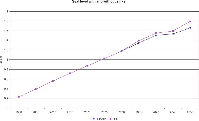
THE MODEL WIAGEM                                                                    283

Furthermore, uncertainty costs, investment decisions under                  emissions growth, radiative forcing, energy production and
uncertainties and forecast uncertainties are only a few                     energy and non-energy related trade. Prices and quantities of
examples of economic uncertainties that make a concrete                     all non-energy data are based on the 1995 GTAP version 4,
cost and benefit evaluation of climate change extremely                     with adjustments to GTAP version 5. This database provides
tentative. Furthermore, socioeconomic behavior is extre-                    trade and production statistics for more than 50 regions and
mely tainted with societal randomness and variability that is               50 commodities. The model covers 26 regions which are
difficult to predict.                                                       aggregated to the 11 trading regions.3
   Most importantly, there is a need to link physical climate                   The model is based on the concept of a general
and biogeochemical system models more effectively, and in                   equilibrium approach. Therefore the model determines
turn improve coupling with descriptions of human activities.                market clearing prices by equalizing economic demand
Currently, human influences are generally treated only                      and supply. It is assumed that all factor markets have perfect
through emission scenarios providing climate system                         competitive behavior, and that demand and supply is cleared
external forcings. More comprehensive human activities                      by market prices (market clearance condition). The output of
models must begin to interact with the dynamics of physical,                domestically produced goods of sector j is an input to the
chemical, and biological sub-systems through a diverse set                  Armington production sector. Armington goods are pro-
of contributing activities, feedbacks, and responses.                       duced by the Armington sector and are used for energy,
   The model WIAGEM is a first attempt to reduce the                        consumption, investment and public production. Further-
above described uncertainties by combining a simplified                     more, profit maximization implies that no activity earns a
climatic and ecologic model with a detailed economic                        positive profit (zero profit condition). Consumption max-
feedback system. The model includes all greenhouse gases                    imization implies that excess demand is always zero, i.e.,
and potential net emissions changes due to sink potential                   means income must be balanced with expenditures (income
from land use change and de-forestation. The climatic model                 balance condition).
is based on general interrelations between energy and non-                      The sectoral disaggregation contains five energy sectors:
energy related emissions, temperature changes and sea level                 coal, natural gas, crude oil, petroleum and coal products and
variations, all inducing substantial market and non-market                  electricity. The dynamic international competitive energy
damage cost economic impacts. The uncertainty about data                    market for oil, coal and gas is modeled by global and
quality is reduced because the model is based on a detailed                 regional supply and demand, while the oil market is
economic database representing a well known and scienti-                    characterized by imperfect competition with the intention
fically accepted economic database. Model and parameter                     that OPEC regions can use their market power to influence
uncertainties are covered by choosing an innovative mod-                    market prices. Energy related greenhouse emissions occur as
eling approach and including parameter sensitivity analysis.                a result of economic and energy consumption and produc-
Of course, not all uncertainties can be covered. However,                   tion activities. Currently, a number of gases have been
there is a need to develop more sophisticated economic                      identified as having a positive effect on radiative forcing [35]
models that cover ecological and climatic interlinkages.                    and are included in the Kyoto protocol as ‘‘basket’’
WIAGEM is a first attempt to fill this gap.                                 greenhouse gases. The model includes three of these gases:
                                                                            carbon dioxide (CO2), methane (CH4) and nitrous dioxide
                                                                            (N2O) which are considered the most influential greenhouse
3. THE MODEL WIAGEM                                                         gases within the short term modeling period of 50 years.
                                                                            Excluding the other gases is not believed to have substantial
WIAGEM is an integrated assessment model integrating an                     impacts on the analysis’ insights.
economy model based on a dynamic intertemporal general                          Because of the short term application of the climate
equilibrium approach combined with an energy market model                   submodel, we consider only the first atmospheric lifetime of
and climatic submodel covering a time horizon of 50 years.                  greenhouse gases, assuming that the remaining emissions
This model is incremented into five-year time steps.2 The                   have an infinite life time. The atmospheric concentrations
basic idea behind this modeling approach is the evaluation of               induced by energy related and non-energy related emissions
market and non-market impacts induced by climate change.                    of CO2, CH4 and N2O have impacts on radiative forcing,
   WIAGEM is benchmarked to the base year 1992.                             influencing potential and actual surface temperature and sea
Benchmark data determine the parameter and coefficients                     level. Market and non-market damages determine regional
of the CES production, demand and utility functions. To                     and overall welfare development.
calibrate the model, we determine the reference level of
                                                                            3
                                                                             The model is written in the computer language GAMS (MPSGE) and
                                                                            solved by the algorithm MILES, see [34]. The model uses the so-called
2
 The model core code is based on an original version developed by Tom       ‘‘Mixed Complementary Format’’ (MCP). The MCP formulation covers the
Rutherford in 1999. A similar model version of the economic model has       transformed non-linear optimization problem into the first order optimiza-
been published by [33]. The model has been modified to include greenhouse   tion conditions. The solver works in a way that the equilibrium condition of
gases, sinks, climate change impacts and induced technological change.      the equations explained later is fulfilled.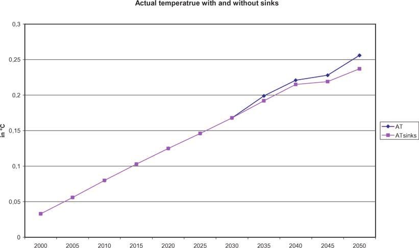
284 CLAUDIA KEMFERT
3.1. Economy each region maximizes lifetime utility from consumption
which implicitly determines the savings level. Firms choose
The economy is represented by an intertemporal computable investment maximizing the present value of their companies.
general equilibrium and multi-regional trade model covering In each region, production of the non-energy macro good
25 world regions aggregated to 11 trading regions linked is captured by an aggregate production function, i.e., each
through bilateral sectoral trade flows. The model is based on production process is described by a production function
GTAP 4.0 data4 from 1995. The world regions are aggregated transforming output by applying a specific technology. The
to the following 11 trading regions (see Tables 1 and 2). factor inputs could be substituted against each other
The economic structure of each region consists of five depending on the ‘‘nesting structure’’ of the CES production
energy sectors: (1) coal, (2) natural gas, (3) crude oil, (4) function. CES production functions use different ‘‘nesting
petroleum and coal products and (5) electricity and industrial levels’’ of input combinations (see Fig. 1). At different
sectors, agriculture and services. Because of the intertemporal levels, input composites could be substituted against other
optimization framework, a savings good sector is included. input factors. Goods are produced for the domestic and
The aggregated factors for production include land, labor and export market. Production of the energy aggregate is
capital. described by a CES function reflecting substitution possibi-
All products are demanded by intermediate production, lities for different fossil fuels (i.e., coal, gas, and oil), capital,
exports, investment and a representative consumer; market and labor representing trade off effects with a constant
actors behave within a full competition context. Consump- substitution elasticity. Fossil fuels are produced from fuel-
tion and investment decisions are based on rational point specific resources and the non-energy macro good subject to
expectations of future prices. The representative agent for a CES technology. Energy efficiency is improved endogen-
ously by increased expenditures in R&D. That means, in the
Table 1. World regions. CES production function, energy productivity is endogen-
ously influenced by changes in R&D expenditures.
Regions The CES production structure follows the concept of
ASIA India and other Asian Countries (Republic of Korea,
ETA-MACRO5 combining nested capital and labor at lower
Indonesia, Malaysia, Philippines, Singapore, Thailand, levels. Energy is treated as a substitute of a capital labor
China, Hong Kong, Taiwan) composite determining (together with material inputs)
CHN China overall output (see Fig. 1). Energy productivity is increased
CAN Canada, New Zealand and Australia endogenously by increased R&D expenditures.
EU15 European Union
JPN Japan
To fulfill the zero profit condition, producers minimize
LSA Latin America (Mexico, Argentina, Brazil, production costs to get a certain value of output. In other
Chile, Rest of Latin America) words, at any point the profit function gives the maximum
MIDE Middle East and North Africa profit while costs are minimized. Markets are perfectly
REC Russia, Eastern and Central European Countries competitive, output and factor prices are fully elastic. The
ROW Other Countries (Rest of the World)
SSA Sub Saharan Africa
representative producer of sector j ascertains the CES profit
USA United States of America function6
Y
Y
1dx 1
ðpÞ ¼ ½adx
j ðpj þ ð1 adx
j Þpfx
1dx 1dx
Table 2. Sectoral classification.
i
h
Sectors
am pm1
j
klem
þ ð1 a m
Þ EPej pe1
j
kle
þ
COL Coal
1kl
CRU Crude Oil þ ð1 EPej Þ½akj ðprk
j Þ þ
GAS Natural Gas
1klem
1kle i
1
EGW Electricity 1klem
1kle
OIL Petroleum and Coal Products þ ð1 akj Þðplj Þ1kl 1kl ð1:1Þ
ORE Iron and Steel
CRP Chemical Rubber and Plastics
5
NFM Non Ferrous Metals CES production functions can be based on different combinations of input
NMM Non Metal mineral Products factors. For example, at the very first level a capital energy composite could
AGR Agriculture be substituted against a labor input, whereas at the second level capital can
PPP Pulp and Paper be substituted against energy (which is mostly a composite of non-electric
TRN Transport Industries and electric energy). [37] shows an overview of different CES production
Y Other Manufactures and Services functions and their nesting options.
6
CSG Savings Good In the mathematical description, we refer to the dual approach, i.e., we
show the cost minimization where the independent variable is the price and
not the quantity as in the primal case. For further explanations about the
4
See [36]. theoretical framework to determine the general equilibrium, see [38].THE MODEL WIAGEM 285
Fig. 1. Production structure of sector j in region r.
with: CES: Constant elasticity of substitution
EPEj;t : Endogenous energy productivity
Yj : Profit function of sector j7
Yj: Activity level of production sector j With EPEj;t ¼ j;t
E
KR & Dj;t as increase of energy produc-
adx
j : Domestic production share of total production by tivity. R&D expenditures (KR&D) improve innovations in
sector i more energy efficient technologies.8 parameterizes the
akj : Value share of capital within capital-energy efficiency of research and development.
composite A representative agent for each region maximizes its
alj : Value share of labor within capital-energy-labor region’s discounted utility over the model’s time horizon (50
aggregate years). This is done under budget constraints equating the
amj : Value share of material within capital-energy-labor present value of consumption demand to the present value of
material aggregate wage income, initial capital stock, present value of rents on
pj: Price of domestic good j fossil energy production, and tax revenue. In each period,
pfx: Price of foreign exchange (exchange rate) households face the choice between current and future
prk: Price of capital consumption which can be purchased via savings. The trade-
pej : Price of energy off between current consumption and savings is given by a
pmj : Price of material=land constant intertemporal substitution elasticity. Producers
pl: Price of labor invest as long as the marginal return on investment equals
dx: Elasticity of transformation between production for the marginal cost of capital formation. The rates of return are
the domestic and production for the export market determined by uniform and endogenous world interest rates
ke: Substitution elasticity between capital and energy such that the marginal productivity of a unit of investment
kle: Substitution elasticity between labor, capital, and and a unit of consumption is equalized within and across
energy composite countries. The primary factors capital, labor, and energy are
klem: Substitution elasticity between material and labor, combined to produce output in period t. In addition, some
capital, and energy composite energy is delivered directly to the final consumer. Output is
CET: Constant elasticity of transformation separated into consumption and investment, and investment
enhances the (depreciated) capital stock of the next period.
7
The notation with the subscript Y is used to consider the activity subset
which is represented by production Y. Because of the zero profit condition,
8
this equation must be equalized to zero. We follow theoretic and applied approaches of [39], [40] or [41].286 CLAUDIA KEMFERT
Capital, labor, and the energy resources earn income which growth rate constraint of sectoral investment in the terminal
is spent on consumption or saved. Savings equals investment period:
through the usual identity. Increased protection costs of
climate change and R&D expenditures lower other Ij;T Cj;T
gKTþ1 ¼ ¼ ð1:5Þ
economic investments (crowding out). Ij;T1 Cj;T1
Sectoral capital stocks depreciate at a constant rate and
are enlarged by investments which cover both investment to Labor is supplied by households and demanded by firms; all
protect against climate change and R&D investment. Capital households are confronted with a specific time quota to be
evolution is assumed to be determined by a specific time lag spent for labor or leisure. This labor–leisure decision is
which is represented by a capital survival share . Capital is determined by net wages ensuring a price elastic labor
used for production with a capital price pKt and a capital supply. One representative agent by each region demands a
9 composite consumption good produced by combining the
utility price of pRK
t , and is depreciated by rate .
Armington good and household energy aggregate good
Y
K
according to a CES configuration. end describes the
ðpÞ ¼ pkpþ1 þ prk
t
t
elasticity of substitution between the composite macro good
and energy aggregate. Aggregate end-use energy comprises
8 ¼ ð1 Þ ; ¼ þ#
oil, gas, and coal with an interfuel elasticity of substitution
¼ prk
t prk
þ #prk
# ptct pR&D
t equal to one. Backstop fuel is a perfect substitute for the
8 þ#¼ ð1:2Þ energy aggregate. Purchase of the good is financed from the
value of the household’s endowments of labor, capital,
with: energy-specific resources, and revenue from any carbon tax
QK or permit prices, respectively (see Fig. 2).
t : Profit function of activity K in time period t
Kt : Activity level of capital in period t Mathematically, this dependence can be written:
pkt : Price of capital in period t 11
prk Y
CG X cg
t : Price of capital services in period t c
cg cg hh 1C a 1C
ðpÞ ¼ p aE ðpE Þ þ ai ðpi Þ
: Capital survival share i
: Depreciation rate
ð1:6Þ
: Time solution parameter
, #: Time lag parameter
with:
ptcrt : Price of regional protection costs QCG
pR&D
t : Price of regional R&D investments : Profit function for consumption activity CG
pcg : Price of consumption good
Investments are produced by Leontief technology:
pai : Price of Armington good i
Y
I X acg
E : Value share of energy aggregate in final demand
ðpÞ ¼ pktþ1 aij paj;t ð1:3Þ c : Substitution elasticity between energy and the non-
tþ1 j energy Armington composite in the consumption
QI sector
t: Profit function for investment activity I in time period t
aij : Value share investment of good j acg
i : Value share of non-energy good in final demand
paj;t : Price of Armington good j in time period t CG: Activity level of real consumption good production
It : Activity level of investments in period t Domestic and imported varieties of non-energy goods for all
R&D investments follow the same determination: domestic market buyers are treated as incomplete substi-
tutes. This is represented by a CES Armington10 aggregation
Y
R&DI X function providing a constant substitution elasticity. With
ðpÞ ¼ pKtþ1 aR&DI
j pR&DA
j;t respect to energy trade, fossil fuels are treated as perfect
tþ1 j
X substitutes, and net trade cannot be cross-transferred.
ITOT ¼ It þ R&Dt ð1:4Þ International capital flows reflect borrowing and lending at
j the world interest rate, and are endogenous subject to an
The model solves for a finite time horizon. Because of that, intertemporal balance of payments constraint assuming no
we need to include a steady state condition to determine changes in net indebtedness over the entire model horizon.
capital in the terminal period. We introduce terminal capital
10
as an additional variable for each capital stock. We assume a In contrast to the assumption of homogenous goods that can be fully
substituted internationally by a Heckscher-Ohlin framework, we assume
that international traded goods cannot be perfectly substituted, i.e., these
9
As with the previous notation, we use the zero profit hypothesis for capital goods are treated as imperfect substitutes. This is represented by an
activity K. Armington trade approach.THE MODEL WIAGEM 287
Fig. 2. Final demand structure.
The profit function of Armington production is specified The intertemporal balance of payment condition determines
by: the equivalence of the sum of exports and balance of payments
and the sum of imports. This means that potential trade deficits
Y
A
1
ðpÞ ¼ paj ½aaj p1 DM
þ ð1 aaj ÞðpfxÞ1DM 1DM
ð1:7Þ or surpluses must be equalized over the entire time period. This
j
j condition represents the model’s basic closure.
with: 3.2. Energy
QA
j : Profit function for the production of the Armington
good j WIAGEM includes four energy production sectors, one non-
paj : Price of Armington good j energy sector and three fossil fuel sectors traded internation-
aaj : Domestically produced good j value share of domestic ally for oil, gas and coal. Coal production in the OECD and
and import good aggregate gas production in Russia grow with energy demand at
pfx: Price of foreign exchange (exchange rate) constant prices. The elasticity of substitution between the
DM : Substitution elasticity between domestic and imported resource input and non-energy inputs is calibrated to meet a
good given price elasticity of supply. Exhaustion leads to rising
Aj: Armington activity level fossil fuel prices at constant demand quantities. The carbon-
free backstop technology establishes an upper boundary on
Key model parameters cover Armington elasticities, back- the world oil price; this backstop fuel is a perfect substitute
stop costs and oil supply elasticities. Within the default or for the three fossil fuels and is available in infinite supply at
BAU scenario, all key parameters are adopted as demon- one price calculated to be a multiple of the world oil price in
strated in Table 3. the benchmark year. Demand elasticities depend on backstop
technologies when low backstop cost demand elasticities are
Table 3. Overview of key parameters. high and vice versa.
A composite energy good is produced by either conven-
Type of Elasticity Value
tional fossil fuels – oil, gas, and coal – represented by a nested
Fossil Fuel Supply CES technology (with an elasticity of interfuel substitution
Coal .5 fuel) or from a backstop source with Leontief technology
Gas 1.2 structures. Oil and gas can be substituted by an elasticity of
Oil .3
substitution twice as large as the elasticity between their
Armington aggregate and coal. The energy good production is
Elasticity of Substitution Domestic vs. Imported Goods 4 determined by industry and household final demand.
Elasticity of Transformation Exports vs. Domestic Sales 8
Production Elasticities Y
E
ele1ele oil oil 1fossil
Interfuel Elasticity of Substitution ðpÞ ¼ pej EPej;t ½aele
j pj þ ð1 aele
j Þ aj ðpj Þ þ
Final demand .5 j
Industry: þ agas gas 1fossil
j ðpj Þ þ acoa hco hco 1coa
j ½aj ðpj Þ þ
Oil=Gas 2
1fossil 1ele 1
Coal=Oil=Gas 1 sco 1coa
Elasticity of Substitution Energy Aggregate vs. .5
þ asco
j ðpj Þ
1coa 1fossil 1ele
Primary Factors KLM pET EMISSj ð2:1Þ288 CLAUDIA KEMFERT
With: Emission limits can be reached by domestic action or by
QE trading Annex B emission permits initially allocated
j : Profit function for the production of energy
according to regional commitment targets. Those countries
aele
j : Electricity value share of energy aggregate by meeting the Kyoto emissions reduction target stabilize their
sector j mitigated emissions at the 2010 level.11
aoil
j : Oil value share of fossil energy aggregate by According to regional abatement costs, countries sell or
sector j buy emission permits. Countries facing high abatement costs
agas
j : Gas value share of fossil energy aggregate by above permit prices will purchase emission permits, regions
sector j with marginal abatement costs lower than the permit price
ahco
j : Hard coal value share of coal aggregate by sector will sell emission licenses. Revenues from permit sales are
j refunded as a lump sum back to the abating country’s
asco
j : Soft coal value share of coal aggregate by sector j representative consumer. It must be stressed that problems
ele: Substitution elasticity between electricity and concerning concrete implementation of the flexible mechan-
fossil energy isms and emissions trading scheme such as compliance,
fossil: Substitution elasticity between fossil energy early crediting and deception influencing permit prices are
inputs neglected within the modeling context.
coa: Substitution elasticity between hard and soft coal
efjoil;co2 : CO2 share of oil in sector j 3.3. Climate
efjgas;co2 : CO2 share of gas in sector j
efjhco;co2 : CO2 share of hard coal in sector j The model comprises three of the most important anthro-
efjsco;co2 : CO2 share of soft coal in sector j pogenic greenhouse gases: carbon dioxide (CO2), covering
pEP: Price emissions permits over 80 percent of total forced radiation by anthropogenic
Ej: Activity level of energy production greenhouse gases, methane (CH4) and nitrous oxide (N2O).
EMISS Sectoral GHG emissions allowances Primarily due to human activities, the concentration of these
Demanded energy by households is produced by a CES gases in the earth’s atmosphere have been increasing since
function: the industrial revolution.
In WIAGEM, we consider the relationship between man-
" #11 eg
YE X eg
made emissions and atmospheric concentrations and their
ðpÞ ¼ pehh aei;hh ðpai þ aei pe Þ1 ð2:2Þ resulting impact on temperature and sea level. Because of
hh i¼eg the 50-year short term analysis lasting until 2050, we neglect
with: classes of atmospheric greenhouse gas stocks with different
atmospheric lifetimes (usually modeled by the impulse
aei;hh : Value share of energy good i of household response function) and reduced forms of the carbon cycle
pehh : Price of energy by household demand model developed by [42] and applied by [43]. Energy and
eg: Substitution elasticities between energy goods non-energy related atmospheric concentrations of CO2, CH4
Ehh: Activity level of energy production by household and N2O have an impact on forced radiation relative to their
The intertemporal optimal dynamic allocation is character- base year levels. Energy related emissions are calculated
ized by a steady state growth path. This means that all sizes according to the energy development of each period. Energy
must rise by a common growth rate in order to reach related CO2 emissions are considered according to the
equilibrium conditions. In the long run, conventional energy emissions coefficients of the EMF group (see Table 4).
(i.e., fossil fuels) are typified by exhaustion, thus increasing Energy related CH4 emissions are determined by the CH4
resource prices. We assume that within future time periods a emissions coefficients of gas and coal production in billions
carbon-free backstop technology will be developed and of tons of CH4 per exajoule gas and coal production; the
utilized as a substitute for conventional energy. As a result, a coefficients are taken from the MERGE model 4.0 [44].
carbon-free backstop technology can be utilized within Tables 5 and 6 show the regional emission coefficients.
future times at price f BS $=t CO2. Zero profit condition is
determined by:
Y
BS Table 4. CO2 coefficients.
¼ pe pCG f BS ð2:3Þ
Coal Oil Gas
with: CO2 coefficients in billions 0.2412 0.1374 0.1994
CG
p : Price of consumption good of metric tons=exaj.
f BS: Costs of carbon-free energy supply
BS: Activity level of backstop technology 11
This can be referred to as the ‘‘Kyoto Forever’’ scenario.THE MODEL WIAGEM 289
Table 5. Emissions coefficients in billions of tons of CH4 per exajoule gas Table 7. Non-energy related emissions in millions of tons-1990; source:
production. (source: MERGE 4.0). MERGE 4.0, [45] and [46].
USA EU15 JPN CNA FSU CHN MIDE ASIA ROW USA EU15 JPN CNA FSU CHN MIDE ASIA ROW
2000 0.187 0.493 0.000 0.225 1.005 1.170 1.377 0.468 0.982 CH4 25.8 15 1 5 7 43.2 0 46 132
2010 0.168 0.413 0.000 0.222 0.823 0.955 1.121 1.121 0.805 N2O 1.1 0.8 0.1 0.3 0.3 0.7 0.2 0.5 1.7
2020 0.149 0.333 0.000 0.190 0.641 0.740 0.864 0.864 0.627
2030 0.131 0.253 0.000 0.158 0.458 0.524 0.607 0.607 0.449
2040 0.112 0.173 0.000 0.126 0.276 0.309 0.350 0.350 0.271
Table 8. Potential sinks enhancement in 2010 in million of tons of carbon;
2050 0.094 0.094 0.000 0.094 0.094 0.094 0.094 0.094 0.094
source: MERGE 4.024.
USA EU15 JPN CNA FSU CHN MIDE ASIA ROW
Table 6. Emissions coefficients in billions of tons of CH4 per exajoule coal
production. (source: MERGE 4.0)23. Sinks 2010 50 17 0 50 34 25 25 13 250
24
USA EU15 JPN CNA FSU CHN MIDE ASIA ROW Note. See [49].
2000 0.354 0.196 0.000 0.371 0.512 0.963 0.000 0.117 0.356
2010 0.354 0.196 0.000 0.371 0.512 0.963 0.000 0.117 0.356
2020 0.354 0.196 0.000 0.371 0.512 0.963 0.000 0.117 0.356
function to an instantaneous atmospheric injection is
2030 0.354 0.196 0.000 0.371 0.512 0.963 0.000 0.117 0.356 expressed as the weighted sum of the exponentials:
2040 0.354 0.196 0.000 0.371 0.512 0.963 0.000 0.117 0.356
2050 0.354 0.196 0.000 0.371 0.512 0.963 0.000 0.117 0.356 X
5
GðtÞ ¼ ai exp
23 i¼1
Note. One model version covers further time periods until 2100. We
assume the same projections until 2100. P
where ai represents scaling factors ai ¼ 1 and the decay
constraints.
Non-energy related emissions cover parts of the CH4 The atmospheric stock of CH4 and N2O in year tþ1
emissions and N2O emissions.12 The global carbon dioxide equals the fraction of the stock in year t remaining in the
emissions baseline pathway is assumed to start from 6 to 11 atmosphere additional to new emissions:
billion tons of carbon in 2030 which is roughly consistent SG;tþ1 ¼ kG SG;t þ EG;t
with the carbon emissions projections of the IPCC reference
case of medium economic growth [35]. With SG,t as the stock of gas G in year t and kG as retention
Additionally, net changes in greenhouse gas emissions factor for gas G and Eg,t as emission in year t.15
are covered from sources and removal by sinks resulting The atmospheric concentration of different greenhouse
from human-induced land use change and forest activities gases have the following impact on radiative forcing relative
such as aforestation, reforestation and deforestation. We use to their base level [50]:
potential sinks enhancements as measured by the [35] and CO2
used in MERGE 4.0:13 FCO2 ¼ 6:3ln ð3:2Þ
CO20
Total emissions are therefore determined by:
X X
TOTEMr;t ¼ Er;t þ NonEr;t Sr;t ð3:1Þ FCH4 ¼ 0:036ðCH40:5 CH40:5
0
Þ f ðCH4 ; N2 OÞþ
GHG GHG
þ f ðCH40 ; N2 O0 Þ ð3:3Þ
with TOTEM indicating the total emissions per region and
time period, and Er,t as regional emissions per time period. FN2 O ¼ 0:14ðN2 O0:5 N2 O0:5
0 Þ f ðCH40 ; N2 OÞþ
Non-energy related emissions are countered for each
þ f ðCH40 ; N2 O0 Þ ð3:4Þ
greenhouse gas, regional and time period. Sinks (Sr,t) reduce
total emissions.14 with F measured in Wm2 as changes in radiative forcing
Atmospheric concentrations of CO2, CH4 and N2O have of each greenhouse gas corresponding to a volumetric
impacts on the forced radiation relative to the base level. concentration change for each greenhouse gas relative to the
Carbon emissions are divided into five classes, each with base level. The CH4N2O interaction term is determined by:
different atmospheric lifetimes. The impulse response
f ðCH4 ; N2 OÞ ¼ 0:47lnb1 þ 2:01 105 ðCH4 N2 OÞ0:75 þ
12
þ 5:31 1015 CH4 ðCH4 N2 OÞ1:52 c
See Table 7.
13
We follow the approach of [47] that additional sinks enhancement ð3:5Þ
activities are costless. An assessment of different sink options analyses are
provided by [48], see Table 8.
14 15
This also means that the emissions reductions targets are reduced. The Key assumptions about greenhouse gases summarizes Table 9.290 CLAUDIA KEMFERT
Table 9. Summary key assumptions greenhouse gases25. Table 10. Protection costs of one meter sea level rise in $109; source: [1].
Trace Gas CO2 CH4 N2O USA EU15 JPN CNA FSU CHN ASIA MIDE
Atmospheric concentration 280 .8 288 71.38 136 63 10.79 53 171 305 5
Pre-Industrial (ppmv) 353 1.72 310
1992 (ppmv)
with sectoral impacts on agriculture, forestry, water
Energy related emissions
1992 (billions of tons) 6.0 .08 .0001 resources and energy consumption, he covers impacts on
Growth Rate, Post-1992 ecosystems and mortality due to vector borne diseases and
cardiovascular and respiratory disorders. We use the
Non-energy related emissions
1992 (billions of tons) .2 .454 .0139 assessed protection costs and an approximation of potential
Growth rate, Post-1992 0 .8 .2 impacts, i.e., additional costs to the economy lowering other
25
investments (crowding out effect). Protection costs due to
Note. Source: [51] and [52].
sea level rise summarizes Table 10.
We follow the approach of (3) for economic impact
assessment of ecosystem changes:
Total chances of radiative forcing F is obtained by adding yt;r yt;r =yb
Et;r ¼ a Pt;r ð3:9Þ
each greenhouse gas radiative forcing effect. The potential y1990;r 1 þ yt;r =yb
temperature PT is influenced by radiative forcing with d as with E as the value of the loss of ecosystems and y the per
parameter (d ¼ 0.455): capita income and P as population size. and yb are
PT ¼ d F ð3:6Þ parameter ( ¼ 0.5, yb ¼ $20.000).
Impact assessment of vector borne diseases are deter-
Actual temperature is reached by a time lag resulting from mined by:
the lag of potential climate change impacts due to tem-
pertature changes: yc yt;r
mr;t ¼ r Tt
yc ybase;r
ATt1 AT ¼ tlag ðPTt ATt Þ ð3:7Þ
? yt;r yc ð3:10Þ
with tlag as the time lag, ATt measures the actual change in
temperature in year t relative to the base year. with m representing mortality, and , and yc denoting
Because of the short term 50-year analysis, sea level will parameter ( ¼ 1 (0.5–1.5), ¼ 1 (0.5–1.5), yc ¼ $3100
change insignificantly during this time period. However, (2100–4100).
newest calculations estimate a rough linear relationship Furthermore, mortality due to changes in global warming
between temperature changes and sea level variations. are measured:
Assuming that sea level will vary by 7 cm with every 1 C M ¼ þ TB ð3:11Þ
temperature change (s ¼ 7), we calculate minor sea level
where M denotes the change in mortality due to a one
changes caused by actual temperature changes. Sea level
degree increase in global warming, Tb as current temperature
variations are determined by the very rough estimates of a
and and are parameter.
linear relationship between actual temperatures:16
Furthermore, we take into account Tol’s approach to
SL ¼ s AT ð3:8Þ determine demand for space heating (SH) and space cooling
Impacts of climate change cover market and non-market energy (SC):
damages; the former comprise all sectoral damages, " Y
t
yt;r Pt;r
production impacts, loss of welfare etc., while the latter SHt;r ¼ ar Tt EPs;r ð3:12Þ
yt;1990 Pt;1990
contain ecological effects such as biodiversity losses, s¼1990
migration, and natural disasters. To assess impacts by
climate change, we follow Tol’s approach [3] to cover yt;r
"
Pt;r Y
t
impacts on forestry, agriculture, water resources and SCt;r ¼ ar Tt EPs;r ð3:13Þ
yt;1990 Pt;1990 s¼1990
ecosystem changes as an approximation of a linear relation-
ship between temperature changes, per capita income or Total damages are assessed by the following relation:
GDP and protection costs due to sea level increase. Tol [3] yrt
estimates climate change vulnerability covering a compre- DAMtr ¼ r
t PTt þ PCtr ð3:14Þ
yr0
hensive evaluation of diverse climate change impacts. Along
with DAM as total impacts (damages), and are param-
16
These estimates are based on assumptions by the climate model NICCS, eters (varying from .5 to 1.5), PC represents the sectoral
[43] and [53]. protection costs due to sea level rise.THE MODEL WIAGEM 291
Fig. 3. Regional greenhouse gas emissions.
3.4. Climate Change and Ecological Fig. 4). Because of the time deceleration of response impacts
Impact Assessment by potential and actual temperature changes ranging from
0.15 to 0.25 C from 2030 to 2050, the inclusion of sinks
This section describes some basic model results. The model causes comparatively marginal actual temperature declines
horizon encompasses 50 years, solving problems in 5-year after 2030.
increments. By including all greenhouse gases (as described Because of the assumed linearity between temperature
in Section 2), total GHG emissions increase from roughly 9 changes and sea level rise, potential sea level increases by
billion tons to 17 billion tons of carbon equivalent emissions 1 cm in 2025 to roughly 1.8 cm in 2050.19 As seen before, the
in 2050 (see Fig. 5 and [50]). incorporation of sinks by land use change and forestry tends
Regional greenhouse gas emissions differ substantially. to lower this increase marginally after 2030. These changes
The inclusion of the other greenhouse gases CH4 and N2O are low in comparison to other projected studies [2] and can
raises reference emissions for the European Union from be explained mainly by the short term time horizon
1.517 in 2010 to 1.894 billion tons of carbon. For the US, the considered and the time deceleration of response impacts
inclusion of sinks lowers the greenhouse gas emissions from (see Figs. 6 and 7).
2.133 to 2.030 in 2010 and 2.686 to 2.496 billion tons of In contrast to many other climate impact assessment
carbon in 2050. Japan has no significant net emissions studies detecting only insignificant economic climate change
changes resulting from sinks inclusion.17 The global CO2 short-term impacts but significant impacts in the long run,
emissions baseline pathway is assumed to start from 6 to we find that climate change impacts also matter within the
12,7 billion tons of carbon in 2050, roughly consistent with next 50 years.20 Model results demonstrate that primarily the
the carbon emissions projections of the IPCC reference case developing countries must accept high welfare losses and
of medium economic growth (see Fig. 3).18 GDP reductions in comparison to a scenario where no
The inclusion of sinks lowers total net GHG emissions to climate change impacts are included. Potential total
roughly 15.5 billion tons of carbon equivalent in 2050 (see damages of climate change are measured in global GDP
percentage covering impacts on forestry, agriculture, water
17
We follow the approach of [47] that additional sinks enhancement
19
activities are cost free. An assessment of different sink options analyses are These estimates are based on assumptions by the climate model NICCS
provided by [48]. [43].
18 20
See [49]. [53] find only marginal climate impacts until 2050.292 CLAUDIA KEMFERT Fig. 4. Regional GHG emissions including sinks. Fig. 5. Total CO2 and GHG emissions with and without inclusion of sinks.
THE MODEL WIAGEM   293

Fig. 6. Actual temperature changes with and without inclusion of sinks.

Fig. 7. Sea level changes with and without the inclusion of sinks, in cm.
294 CLAUDIA KEMFERT
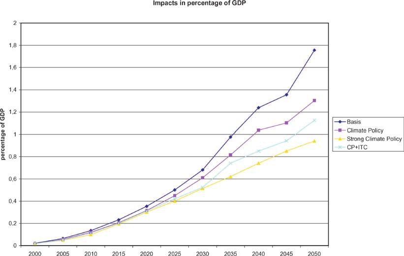
Fig. 8. Impacts of climate change in percentage of global GDP.
resources and ecosystem changes as an approximation of a GDP are lower than if it would not be included. Although the
linear relationship between temperature changes, per capita costs of climate change are higher than economic benefits, a
income or GDP and protection costs due to sea level rise, see strong climate policy that leads to substantial emissions
equation (3.14). Emissions upsurge augments climate reductions could reduce these costs and improve long-term
change impacts through global warming and sea level rise. benefits.
Figure 8 compares the impacts of climate change through the We determine impacts of climate change according to
emissions reductions induced by the Kyoto protocol.21 The equations (3.9) to (3.14). Table 11 summarizes total impacts
emissions reductions prescribed by the Kyoto protocol of climate change and its breakdown into its individual
require a huge economic effort to drastically reduce GHG resulting effects. Developing regions suffer economic
emissions, thus inducing lower economic impacts of climate deficits if climate impacts are included due to their
change measured in GDP percentage. Figure 8 compares the vulnerability and higher percentage impacts of economic
impacts of climate change of a so-called ‘‘business as usual’’ values. These impacts can be explained through different
scenario where no emissions reduction takes place and two effects: First, relatively poor countries must spend a higher
further scenarios where both weak and very strong climate percentage of their income on protection costs. As a
policy is implemented. As can be seen in Figure 8, climate consequence, higher production losses result from decreased
policy implying drastic emisions reductions induces less economic investments. Second (this effect dominates the
impacts, here measured in percentage of GDP. That means economic consequences), fast-growing regions like China
that without any climate policy, economic damages and costs and Asia increase production, resulting in negative climatic
are much higher than related benefits; with increasing and ecological effects. Together with huge population and
greenhouse gas emissions reduction these damages are production growth, these negative impacts augment drasti-
further decreased. The option of technological changes cally until 2050.
through R&D investments could offer better emissions Figure 9 summarizes the total impacts in terms of GDP
reduction opportunities. For that, total impacts in terms of changes in forestry, water, and air conditioning and heating.
The decomposition of these effects demonstrate only
21
We assume a GHG reduction by 5.8% (as was previously intended). negative impacts on forestry for the regions of EasternTHE MODEL WIAGEM 295
Table 11. Impacts of climate change, measured in percentage of GDP (negative, þpositive impacts).
2010 2020 2030 2040 2050
Ecological impacts
JPN 0.018 0.018 0.018 0.018 0.017
CHN 1.585 1.870 1.945 2.139 2.600
USA 0.019 0.019 0.020 0.021 0.021
SSA 1.031 1.039 1.119 1.237 1.293
ROW 0.022 0.037 0.063 0.095 0.134
CAN 0.058 0.051 0.056 0.062 0.066
EU15 0.027 0.027 0.027 0.027 0.037
REC 0.170 0.176 0.231 0.284 0.344
LSA 0.253 0.381 0.630 1.000 1.408
ASIA 1.254 1.937 2.917 3.860 4.964
Vector borne diseases
JPN 0 0 0 0 0
CHN 0.077 0.120 0.185 0.211 0.246
USA 0.000 0.000 0.000 0.000 0.000
SSA 0.080 0.126 0.193 0.221 0.256
ROW 0.000 0.000 0.000 0.000 0.000
CAN 0.000 0.000 0.000 0.000 0.000
EU15 0.000 0.000 0.000 0.000 0.000
REC 0.096 0.143 0.188 0.160 0.147
LSA 0.035 0.055 0.037 0.060 0.111
ASIA 0.080 0.125 0.190 0.217 0.252
Forestry and water, heating and cooling
JPN 0.017 0.021 0.026 0.028 0.029
CHN 0.002 0.003 0.004 0.004 0.004
USA 0.035 0.046 0.053 0.056 0.059
SSA 0.006 0.007 0.008 0.009 0.010
ROW 0.009 0.011 0.014 0.014 0.016
CAN 0.008 0.010 0.012 0.013 0.014
EU15 0.009 0.011 0.014 0.014 0.017
REC 0.049 0.063 0.086 0.102 0.114
LSA 0.002 0.003 0.003 0.004 0.004
ASIA 0.016 0.020 0.026 0.028 0.030
Mortality 0.564 0.600 0.654 0.675 0.703
Sum impacts
JPN 0.565 0.597 0.645 0.665 0.690
CHN 2.223 2.587 2.779 3.021 3.544
USA 0.548 0.574 0.620 0.640 0.665
SSA 1.681 1.771 1.974 2.142 2.262
ROW 0.577 0.627 0.703 0.755 0.821
CAN 0.614 0.641 0.698 0.725 0.756
EU15 0.582 0.616 0.667 0.688 0.723
REC 0.878 0.982 1.160 1.220 1.308
LSA 0.854 1.039 1.324 1.739 2.226
ASIA 1.882 2.642 3.735 4.724 5.889
Europe and Russia and Latin South America. Regions like Emissions reduction as assumed in the latest climate
the USA and Europe boost positive economic effects of change negotiations22 could lead to fewer negative economic
forestry changes. On the other hand, climate change induces impacts. However, these effects are only marginal until
negative impacts to all world regions except China regarding 2050. To deal with uncertainty as mentioned in the previous
water resources. The energy demand for space heating is part of this article, we calculate sensitivity scenarios using
reduced in most of the world regions so that positive impacts parameter variation. Sensitivity calculations show that
in terms of GDP are induced. Contrarily, space heating for
cooling increases due to increased temperature changes. 22
We assume that the USA does not reduce emissions, resulting in a total
This generates negative economic impacts. GHG emissions reduction of only 1.8%.296 CLAUDIA KEMFERT
Fig. 9. Impacts of climate change measured in % of GDP in 2050, mitigation and sensitivity analysis.
results can vary significantly if high or low basic parameter well. The additional inclusion of sinks improves the welfare
are assumed. Total impacts of climate change increase in impacts in comparison to all other scenarios, leading to
high growing regions if parameter , and of equation higher economic impacts. The decomposition of climatic
(3.9) to (3.14) are very high. This can be explained by the effects shows a high share of ecosystem damages.
stronger impact resulting from temperature changes and Vulnerable nations suffer huge economic losses.
income variations.
ACKNOWLEDGEMENTS
4. CONCLUSION
I would like to thank the Ministry of Science and Culture in
Germany for financially supporting this study. I would also
The model WIAGEM is an integrated assessment model
like to thank Alan Manne, Richard Tol, and Bob van der
building on a detailed economic intertemporal general
Zwaan, and two anonymous referees for their very useful
equilibrium model covering 25 world regions and 14 sectors
commentary and suggestions.
of each world region. It contains an energy submodel
representing the international market for oil, coal and gas
and allows a more realistic representation of the oil market in REFERENCES
the sense that OPEC regions can influence the oil market
price with their market power. Technological innovations 1. Tol, R.: Estimates of the Damage Costs of Climate Change, Part II:
improve energy efficiencies endogenously. An integrated Benchmark Estimates. Environ. Resource Econom. 21 (2002a), pp. 47–
73.
assessment of economic, ecological and climate impacts is 2. IPCC: WG II Climate Change 2001: Impacts, Adaptation and
reached through an incorporation of climate and ecologic Vulnerability, 2001.
interlinkages attempting to evaluate economic market and 3. Tol, R.: Estimates of the Damage Costs of Climate Change, Part II:
non-market damages of climate change. Coverage of all Dynamic Estimates. Environ. Resource Econom. 21 (2002b),
GHGs improves the economic welfare impacts especially for pp. 135–160.
4. Prentice, C., Cramer, W., Harrison, S.P., Leemans, R., Monserud, R.A.
OECD regions. Here, not only do the additional options of and Solomon, A.M.: A Global Biome Model Based on Plant Physiology
emissions abatement increase by the inclusion of all and Dominance, Soil Properties and Climate. J. Biogeogr. (1992), pp.
greenhouse gases, but the international price diminishes as 117–134.THE MODEL WIAGEM 297
5. Haxeltine, A., Prentice, I.C. and Creswell, D.I.: A Coupled Carbon and Rayner and E. Malone (eds.): Human Choice and Climate Change:
Water Flux Model to Predict Vegetation Structure. J. Vegetation Sci. An International Social Science Assessment. Batelle Press, USA, 1998.
7(5) (1996), pp. 651–666. 26. Toth, F.L.: Practice and Progress in Integrated Assessments of Cli-
6. Kaplan, J.: Geophysical Applications of Vegetation Modelling. mate Change: A Workshop Overview. Energy Policy 23(4/5) (1995),
Dissertation, Universit€at Lund, Abteilung Pflanzenphysiologie, Lund, 253.
Schweden, 2001, ISBN 91-7874-089-4. 27. Rotmans, J. and van Asselt, M.: Uncertainty Management in Integrated
7. Esser, G., Hoffstadt, J., Mack, F. and Wittenberg, U.: High-Resolution Assessment Modeling: Towards a Pluralistic Approach, ICIS Studies-
Biosphere Model – Documentation. Mitteilungen aus dem Institut f€ur 01-06, 2001.
Pflanzen€okologie der Justus-Liebig-Universit€at Gießen, Gießen, 28. Bernstein, P., Montgomery, W.D.: Global Impacts of the Kyoto
Germany, 1994. Agreement: Results from the MS-MRT Model, Paris, 1999.
8. Kaduk, J.: Simulation der Kohlenstoffdynamik der globalen 29. McKibbin, W. and Wilcoxen, P.: Permit Trading Under the Kyoto
Landbiosph€ are mit SILVAN – Modellbeschreibung und Ergebnisse. Protocol and Beyond. Paris, 1999.
Max-Planck-Institut f€ur Meteorologie, Examensarbeit Nr. 42, 1996, 30. Rutherford, F.T., B€ohringer, C. and Pahlke, A.: Carbon Abatement,
pp. 157. Revenue Recycling and Intergenerational Burden Sharing. The Theory
9. Knorr, W.: Annual and Interannual CO2 Exchanges of the Terrestrial of Markets (1998), pp. 305–323.
Biosphere: Process-Based Simulations and Uncertainties. Global Ecol. 31. Kemfert, C.: Economic Implications of the Kyoto Protocol, Perspec-
Biogeogr. 9 (2000), pp. 225–252. tives of Newest Climate Change Policy Options. Environ. Econom.
10. Knorr, W. and Heimann, M.: Uncertainties in Global Terrestrial (2000).
Biosphere Modeling. Part I: A Comprehensive Sensitivity Analysis 32. Kemfert, C.: Global Economic Implications of Alternative Cli-
with a New Photosynthesis and Energy Balance Scheme. Global mate Policy Strategies. Environ. Sci. Policy 5(5) (2000), pp. 367–
Biogeochem. Cycles 15(1) (2001), pp. 207–225. 384.
11. Maier-Reimer, E. and Hasselmann, K.: Transport and Storage of CO2 in 33. Bernstein, P., Montgomery, W.D. and Rutherford, T.: Global Impacts
the Ocean – An Inorganic Ocean-Circulation Carbon Cycle Model. of the Kyoto Agreement: Results from the MS-MRT Model. Paris,
Clim. Dynam. 2 (1987), pp. 63–90. 1999.
12. Maier-Reimer, E.: The Biological Pump in the Greenhouse. Global 34. Rutherford, T.: MILES: A Mixed Inequality and Non-Linear Equation
Planetary Climate Change 8 (1993), pp. 13–15. Solver. 1993.
13. Sarmiento, L., Orr, J.C. and Siegenthaler, U.: A Perturbation 35. IPCC: Climate Change 1995, The Science of Climate Change.
Simulation of CO2 Uptake in an Ocean General Circulation Model. Contribution of Working Group I to the Second Assessment Report
J. Geophys. Res. 97(3) (1992), pp. 3621–3645. of the IPCC. Cambridge. University Press, Cambridge, 1996, p.
14. Siegenthaler, U. and Oeschger, H.: Predicting Future Atmospheric 572.
Carbon Dioxide Levels. Science 199 (1978), pp. 388–395. 36. McDougall, R.A.: The GTAP 3 Data Base. Center for Global Trade
15. Hasselmann, K., Hasselmann, S., Giering, R., Oca~na, V. and v. Storch, Analysis, Purdue University, 1995.
H.: Sensitivity Study of Optimal CO2 Emission Paths Using a 37. Kemfert, C.: Estimated Substitution Elasticities of a Nested CES
Simplified Structural Integrated Assessment Model (SIAM). Clim. Production Function for Germany. Energy Econom. 20 (1998),
Change 37 (1997), pp. 345–386. pp. 249–264.
16. Meyer, R., Joos, F., Esser, G., Heimann, M., Hooss, G., Kohlmaier, G., 38. Shoven, J. and Whalley, J.: Applying General Equilibrium. Cambridge
Sauf, W., Voss, R. and Wittenberg, U.: The Substitution of High- Surveys of Economic Literature. Cambridge University Press,
Resolution Terrestrial Biosphere Models and Carbon Sequestration in Cambridge, 1992.
Response to Changing CO2 and Climate. Global. Biogeochem. Cycles 39. Goulder, Mathai: Optimal CO2 Abatement in the Presence of Induced
13 (1999), pp. 785–802. Technological Change. J. Environ. Econom. Manage. 39 (2000),
17. Joos, F., Prentice, C., Sitch, S., Meyer, R., Hooss, G., Plattner, K. and pp. 1–38.
Hasselmann, K.: Global Warming Feedbacks on Terrestrial Carbon 40. Buonanno, Carraro, Galeotti: Endogenous Induced Technical
Uptake Under the IPCC Emission Scenarios. in preparation. Change and the Costs of Kyoto. Fondazione Eni Enrico Mattei
18. Hooss, K.G., Voss, R., Hasselmann, K., Maier-Reimer, E. and Joos, (2000).
F.: A Nonlinear Impulse Response Model of the Coupled Carbon 41. Nordhaus: Modeling Induced Innovation in Climate-Change Policy.
Cycle-Climate System (NICCS). Clim. Dynam. 18 (2001), Paper Presented at the IIASA Workshop on Induced Technological
pp. 189–202. Change and the Environment, 1997, Laxenburg.
19. Manne, S.A. and Richels, G.R.: The Kyoto Protocol: A Cost- 42. Maier-Reimer, E. and Hasselmann, K.: Transport and Storage of CO2 in
Effective Strategy for Meeting Environmental Objectives? ACCF the Ocean – An Inorganic Ocean-Circulation Carbon Cycle Model.
Center for Policy Research: Climate Change Policy: Practical Clim. Dynam. 2 (1987), pp. 63–90.
Strategies to Promote Economic Growth and Environmental Quality, 43. Hooss, K.G., Voss, R., Hasselmann, K., Maier-Reimer, E. and Joos,
1998. F.: A Nonlinear Impulse Response Model of the Coupled Carbon
20. Nordhaus, W.D. and Yang, Z.: RICE: A Regional Dynamic General Cycle-Climate System (NICCS). Clim. Dynam. 18 (2001), pp.
Equilibrium Model of Optimal Climate Change Policy. Am. Econom. 189–202.
Rev. 86 (1996), pp. 741–765. 44. Manne, A. and Richels, R.: The Kyoto Protocol: A Cost-Effective
21. Peck, S.C. and Teisberg, T.J.: CETA: A Model for Carbon Emissions Strategy for Meeting Environmental Objectives? 1998.
Trajectory Assessment. Energy J. 13 (1991), pp. 55–77. 45. Schimel, D.S., Enting, I., Heimann, M., Wigley, T.M., Raynaud, D.,
22. Tol, R.: Temporal and Spatial Efficiency in Climate Policy: Applica- Alves, D. and Siegenthaler, U.: CO2 and the carbon cycle. In: J.T.
tions of FUND. Environ. Resource Econom. in press. Houghton , L.G.M. Filho, J. Bruce, H. Lee, B.A. Callander, E. Haites,
23. Edmonds, J.: Climate Change Economic Modeling: Background N. Harris and K. Maskell (eds.): IPCC Report. Climate Change 1994.
Analysis for the Kyoto Protocol. OECD Workshop, Paris, 1998. Radiative Forcing of Climate Change and An Evaluation of the IPCC
24. Dowlatabadi, H. and Morgan, M.G.: Integrated Assessment of Climate IS92 Emission Scenarios. Cambridge University Press, Cambridge,
Change. Science 259 (1993), pp. 1813, 1932. UK, 1994.
25. Dowlatabadi, H. and Rotmans, J.: Integrated Assessment of 46. IEA: Abatement of Methane Emissions, IEA Greenhouse Gas R&D
Climate Change: Evaluation of Models and Other Methods. In S. Program. 1998.You can also read