Chapter 3. Modelling the climate system 3.
←
→
Page content transcription
If your browser does not render page correctly, please read the page content below
Introduction to climate dynamics and climate modelling - http://www.climate.be/textbook

Chapter 3. Modelling the climate system

3.1 Introduction
      3.1.1 What is a climate model ?
      In general terms, a climate model could be defined as a mathematical representation
of the climate system based on physical, biological and chemical principles (Fig. 3.1).
The equations derived from these laws are so complex that they must be solved
numerically. As a consequence, climate models provide a solution which is discrete in
space and time, meaning that the results obtained represent averages over regions, whose
size depends on model resolution, and for specific times. For instance, some models
provide only globally or zonally averaged values while others have a numerical grid
whose spatial resolution could be less than 100 km. The time step could be between
minutes and several years, depending on the process studied.
       Even for models with the highest resolution, the numerical grid is still much too
coarse to represent small scale processes such as turbulence in the atmospheric and
oceanic boundary layers, the interactions of the circulation with small scale topography
features, thunderstorms, cloud micro-physics processes, etc. Furthermore, many
processes are still not sufficiently well-known to include their detailed behaviour in
models. As a consequence, parameterisations have to be designed, based on empirical
evidence and/or on theoretical arguments, to account for the large-scale influence of these
processes not included explicitly. Because these parameterisations reproduce only the
first order effects and are usually not valid for all possible conditions, they are often a
large source of considerable uncertainty in models.
       In addition to the physical, biological and chemical knowledge included in the
model equations, climate models require some input from observations or other model
studies. For a climate model describing nearly all the components of the system, only a
relatively small amount of data is required: the solar irradiance, the Earth’s radius and
period of rotation, the land topography and bathymetry of the ocean, some properties of
rocks and soils, etc. On the other hand, for a model that only represents explicitly the
physics of the atmosphere, the ocean and the sea ice, information in the form of boundary
conditions should be provided for all sub-systems of the climate system not explicitly
included in the model: the distribution of vegetation, the topography of the ice sheets, etc.
      Those model inputs are often separated into boundary conditions (which are
generally fixed during the course of the simulation) and external forcings (such as the
changes in solar irradiance) which drives the changes in climate. However, those
definitions can sometimes be misleading. The forcing of one model could be a key state
variable of another. For instance, changes in CO2 concentration could be prescribed in
some models, but it is directly computed in models including a representation of the
carbon cycle. Furthermore, a fixed boundary in some models, such as the topography of
the ice sheet, can evolve interactively in a model designed to study climate variations on
a longer time scale.
      In this framework, some data are required as input during the simulation. However,
the importance of data is probably even greater during the development phase of the
model, as they provide essential information on the properties of the system that is being
modelled (see Fig. 3.1). In addition, large numbers of observations are needed to test the
validity of the models in order to gain confidence in the conclusions derived from their
results (see section 3.5.2).

                                               59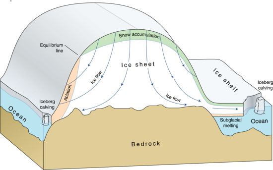
Goosse H., P.Y. Barriat, W. Lefebvre, M.F. Loutre and V. Zunz (2010)

       Many climate models have been developed to perform climate projections, i.e. to
simulate and understand climate changes in response to the emission of greenhouse gases
and aerosols. In addition, models can be formidable tools to improve our knowledge of
the most important characteristics of the climate system and of the causes of climate
variations. Obviously, climatologists cannot perform experiments on the real climate
system to identify the role of a particular process clearly or to test a hypothesis. However,
this can be done in the virtual world of climate models. For highly non-linear systems, the
design of such tests, often called sensitivity experiments, has to be very carefully
planned. However, in simple experiments, neglecting a process or an element of the
modelled system (for instance the influence of the increase in CO2 concentration on the
radiative properties of the atmosphere) can often provide a first estimate of the role of this
process or this element in the system.

      Figure 3.1: Schematic representation of the development and use of a climate
      model.

      3.1.2 Types of models
      Simplifications are unavoidable when designing a climate model as the processes
that should be taken into account range from the scale of centimetres (for instance for
atmospheric turbulence) to that of the Earth itself. The involved time scales also vary
widely from the order of seconds for some waves, to billions of years when analysing the
evolution of the climate since the formation of Earth. It is thus an important skill for a
modeller to be able to select the processes that must be explicitly included compared to
those that can be neglected or represented in a simplified way. This choice is of course
based on the scientific goal of the study. However, it also depends on technical issues
since the most sophisticated models require a lot of computational power: even on the
largest computer presently available, the models cannot be routinely used for periods
longer than a few centuries to millennia. On longer time scales, or when quite a large
number of experiments are needed, it is thus necessary to user simpler and faster models.
Furthermore, it is often very illuminating to deliberately design a model that includes

                                              60
3. Modelling of the climate system
only the most important properties, so as to understand in depth the nature of a feedback
or the complex interaction between the various components of the system. This is also the
reason why simple models are often used to analyse the results of more complex models
in which the fundamental characteristics of the system could be hidden by the number of
processes represented and the details provided.
Modellers have first to decide the variables or processes to be taken into account
and those that will be taken as constants. This provides a method of classifying the
models as a function of the components that are represented interactively. In the majority
of climate studies, at least the physical behaviour of the atmosphere, ocean and sea ice
must be represented. In addition, the terrestrial and marine carbon cycles, the dynamic
vegetation and the ice sheet components are more and more regularly included, leading to
what are called Earth-system models.
Figure 3.2: Types of climate model.
A second way of differentiating between models is related to the complexity of the
processes that are included (Fig. 3.2). At one end of the spectrum, General Circulation
Models (GCMs) try to account for all the important properties of the system at the highest
affordable resolution. The term GCM was introduced because one of the first goals of
these models is to simulate the three dimensional structure of winds and currents
realistically. They have classically been divided into Atmospheric General Circulation
Models (AGCMs) and Ocean General Circulation Models (OGCMs). For climate studies
using interactive atmospheric and oceanic components, the acronyms AOGCM
(Atmosphere Ocean General Circulation Model) and the broader CGCM (Coupled
General Circulation Model) are generally used.
At the other end of the spectrum, simple climate models (such as the Energy
Balance Models, or EBMs, see section 3.2.1) propose a highly simplified version of the
dynamic of the climate system. The variables are averaged over large regions, sometimes
over the whole Earth, and many processes are not represented or accounted for by the
parameterisations. EBMs thus include a relatively small number of degree of freedom.
61Goosse H., P.Y. Barriat, W. Lefebvre, M.F. Loutre and V. Zunz (2010)
EMICs (Earth Models of Intermediate Complexity) are located between those two
extremes. They are based on a more complex representation of the system than EBMs but
include simplifications and parameterisations for some processes that are explicitly
accounted for in GCMs. The EMICs form the broadest category of models. Some of them
are relatively close to simple models, while others are slightly degraded GCMs.
When employed correctly, all the model types can produce useful information on the
behaviour of the climate system. There is no perfect model, suitable for all purposes. This
is why a wide range of climate models exists, forming what is called the spectrum or the
hierarchy of models that will be described in section 3.2. Depending on the objective or
the question, one type of models could be selected. The best type of model to use depends
on the objective or the question. On the other hand, combining the results from various
types of models is often the best way to gain a deep understanding of the dominant
processes in action.
3.2 A hierarchy of models
3.2.1 Energy balance models
As indicated by their name, energy balance models estimate the changes in the
climate system from an analysis of the energy budget of the Earth. In their simplest form,
they do not include any explicit spatial dimension, providing only globally averaged
values for the computed variables. They are thus referred to as zero-dimensional EBMs.
The basis for these EBMs was introduced by both Budyko (1969) and Sellers in (1969).
Their fundamental equation is very similar to those analysed in sections 2.1.1 and 2.1.5:
Changes in heat storage = absorbed solar radiation - emitted terrestrial radiation
∂Ts ⎛ ⎞
= ⎜ (1 − α p ) 0 − A ↑ ⎟
S
CE (3.1)
∂t ⎝ 4 ⎠
where, as in Chapter 2, CE is the effective heat capacity of the media (measured in J m-2
K-1), Ts the surface temperature, t the time, αp the planetary albedo, S0 the Total Solar
Irradiace (TSI) and A↑ the total amount of energy that is emitted by a 1 m2 surface of the
Earth. A↑ could be represented on the basis of the Stefan-Boltzmann law, using a factor
τa to represent the infrared transmissivity of the atmosphere (including the greenhouse
gas effect), as.
A ↑= εσTs4τ a (3.2)
where ε is the emissivity of the surface. Using an albedo of 0.3, an emissivity of 0.97, and
a value of τa of 0.64 leads to an equilibrium temperature Ts=287K, which is close to the
observed one. In some EBMs, Eq. 3.2 is linearised to give an even simpler formulation of
the model. On the other hand, τa and αp are often parameterised as a function of the
temperature, in particular to take into account the fact that cooling increases the surface
area covered by ice and snow, and thus increases the planetary albedo.
In order to take the geographical distribution of temperature at the Earth’s surface
into account, zero-dimensional EBMs can be extended to include one (generally the
latitude) or two horizontal dimensions (Fig. 3.3). An additional term Δtransp is then
included in Eq. 3.1 representing the net effect of heat input and output associated with
horizontal transport:
623. Modelling of the climate system
∂Ts,i ⎛ ⎞
= ⎜ (1 − α p ) 0 − A ↑ ⎟ + Δtransp
S
CE (3.3)
∂t ⎝ 4 ⎠
An index i has been added to the surface temperature to indicate that the variable
corresponds to the region i. The simplest form for the transport is to treat it as a linear
function of temperature, but more sophisticated parameterisations are also used,
including, for instance, a diffusion term.
Figure 3.3: Representation of a one-dimensional EBM for which the temperature Ti
is averaged over a band of longitude.
Box models have clear similarities to EBMs as they represent large areas or an
entire component of the system by an average which describes the mean over one “box”.
The exchanges between the compartments are then parameterised as a function of the
characteristics of the different boxes. The exact definition of the boxes depends on the
purpose of the model. For instance, some box models have a compartment for the
atmosphere, the land surface, the ocean surface layers and the deep ocean, possibly
making a distinction between the two hemispheres. Others include additional components
allowing a description of the carbon cycle and thus have boxes corresponding to the
various reservoirs described in section 2.3.
3.2.2 Intermediate complexity models
Like EBMs, EMICs involve some simplifications, but they always include a
representation of the Earth’s geography, i.e. they provide more than averages over the
whole Earth or large boxes. Secondly, they include many more degrees of freedom than
EBMs. As a consequence, the parameters of EMICs cannot easily be adjusted to
reproduce the observed characteristics of the climate system, as can be done with some
simpler models.
The level of approximation involved in the development of the model varies widely
between different EMICs. Some models use a very simple representation of the
63Goosse H., P.Y. Barriat, W. Lefebvre, M.F. Loutre and V. Zunz (2010)
geography, with a zonally averaged representation of the atmosphere and ocean. A
distinction is always made between the Atlantic, Pacific and Indian basins (Fig. 3.4)
because of the strong differences between them in the circulation (see section 1.3.2). As
the atmospheric and oceanic circulations are fundamentally three-dimensional, some
parameterisations of the meridional transport are required. Those developed for EMICs
are generally more complex and physically based than the ones employed in one-
dimensional EBMs.
On the other hand, some EMICs include components that are very similar to those
developed for GCMs, although a coarser numerical grid is used so that the computations
proceed fast enough to allow a large number of relatively long simulations to be run.
Some other components are simplified, usually including the atmosphere because this is
the component that is most depending on computer time in coupled climate models.
Figure 3.4: Schematic illustration of the structure of the climate model of
intermediate complexity MOBIDIC that includes a zonally averaged atmosphere, a
3-basin zonal oceanic model (corresponding to the Atlantic, the Pacific and the
Indian Oceans) and simplified ice sheets. More details about this model are
available at http://www.astr.ucl.ac.be/index.php?page=MoBidiC%40Description.
3.2.3 General circulation models
General circulation models provide the most precise and complex description of the
climate system. Currently, their grid resolution is typically of the order of 100 to 200 km.
As a consequence, compared to EMICs (which have a grid resolution between 300 km
and thousands of kilometres), they provide much more detailed information on a regional
scale. A few years ago, GCMs only included a representation of the atmosphere, the land
surface, sometimes the ocean circulation, and a very simplified version of the sea ice.
Nowadays, GCMs take more and more components into account, and many new models
643. Modelling of the climate system
now also include sophisticated models of the sea ice, the carbon cycle, ice sheet dynamics
and even atmospheric chemistry (Fig. 3.5).
Figure 3.5: A simplified representation of part of the domain of a general
circulation model, illustrating some important components and processes. For
clarity, the curvature of the Earth has been amplified, the horizontal and vertical
coordinates are not to scale and the number of grid points has been reduced
compared to state-of-the-art models.
Because of the large number of processes included and their relatively high
resolution, GCM simulations require a large amount of computer time. For instance, an
experiment covering one century typically takes several weeks to run on the fastest
computers. As computing power increases, longer simulations with a higher resolution
become affordable, providing more regional details than the previous generation of
models.
3.3 Components of a climate model
3.3.1 Atmosphere
The basic equations that govern the atmosphere can be formulatedG as a set of seven
equations with seven unknowns: the three components of the velocity v (components u,
v, w), the pressure p, the temperature T, the specific humidity q and the density. The
seven equations, written for the atmosphere, are:
65Goosse H., P.Y. Barriat, W. Lefebvre, M.F. Loutre and V. Zunz (2010)
G G
(1-3) Newton’s second law (momentum balance, i.e. F = ma , force equals mass times
acceleration),
G JG G
dv 1G G G
= − ∇p − g + Ffric − 2Ω × v (3.4)
dt ρ
In this equation, d /dt is the total derivative, including a transport term,
d ∂ GG
= + v .∇ (3.5)
dt ∂t
G G
g is the apparent gravity vector (i.e. taking the centrifugal force into account), Ffric is the
JG
force due to friction, and Ω is the angular velocity vector of the Earth (the last term is the
Coriolis force)
(4) The continuity equation or the conservation of mass
∂ρ G G
= −∇. ( ρv ) (3.6)
∂t
(5) The conservation of the mass of water vapour
∂ρ q G G
= −∇.( ρvq ) + ρ (E − C ) (3.7)
∂t
where E and C are evaporation and condensation respectively
(6) The first law of thermodynamics (the conservation of energy)
dT 1 dp
Q = Cp − (3.8)
dt ρ dt
where Q is heating rate per unit mass and Cp the specific heat
(7) The equation of state
p = ρ RgT (3.9)
Before these equations are used in models some standard approximations have to be
performed. For instance, assuming hydrostatic equilibrium, which is a good
approximation at the scale of GCMs, provides a considerable simplification of the
equation of motion along the vertical. Secondly, the quasi-Boussinesq approximation
states that the time variation of the density could be neglected compared to the other
terms of the continuity equation, filtering the sound waves. However, supplementary
equations for the liquid water content of atmospheric parcels or other variables related to
clouds are often added to this set of equations.
Unfortunately, these seven equations do not form a closed system. First, the
frictional force and the heating rate must be specified. Computing the heating rate, in
particular, requires a detailed analysis of the radiative transfer in the atmosphere,
663. Modelling of the climate system
accounting for both the longwave and the shortwave radiation in the atmospheric
columns (see Fig. 3.5), as well as of the heat transfers associated with evaporation,
condensation and sublimation. The influence of clouds in these processes is usually a
source of considerable uncertainty. This part of the model is commonly referred to as the
model “physics” while the calculation of the transport is called the “dynamics”.
Secondly, as discussed in section 3.1.1, the models can only adequately resolve some of
the processes that are included in the equations. The important processes that occur at
scales that could not be resolved by the model grid must thus be parameterised,
introducing new terms into the equations 3.5, 3.7 and 3.8. The boundary conditions of the
equations describing the interactions between the atmosphere and the other components
of the climate system also need to be specified (see section 3.3.7).
3.3.2 Ocean
The major equations that govern the ocean dynamics are based on the same
principles as the equations for the atmosphere. The only significant difference is that the
equation for the specific humidity is not required for the ocean, while a new equation for
the salinity needs to be introduced. The equation of state is also fundamentally different.
Unlike the atmosphere, there is no simple law for the ocean and the standard equation of
state is expressed as a function of the pressure, the temperature and the salinity as a long
polynomial series.
It is much easier to compute the heating rate in the ocean than in the atmosphere. In
addition to the heat exchanges at the surface, the only significant heat source in the ocean
is the absorption of solar radiation. This is taken into account in the model through an
exponential decay of the solar irradiance. The situation for salinity is even more
straightforward, as there is no source or sink of salinity inside the ocean. The equations
governing these two variables are thus relatively simple:
dT
= Fsol + Fdiff (3.10)
dt
dS
= Fdiff (3.11)
dt
where Fsol is the absorption of solar radiation in the ocean. Eq. 3.10 does not apply to the
in situ temperature, but the potential temperature in order to account for the effect of
the compressibility of seawater. The difference between those two temperatures is
relatively low in the upper ocean, but it can reach several tenths of a degree in the deeper
layers, an important difference in areas where the gradients are relatively small (see
section 1.3.3.2).
In Eqs. 3.10 and 3.11, in contrast to section 3.3.1, we have explicitly added a term
to the right hand side representing the influence of the processes at scales that cannot be
included in the model. As small-scale processes tend to mix properties, they are generally
modelled as a diffusion term Fdiff. In its simplest form, a Laplacian formulation is
retained. This is also often the formulation selected for the friction term (in Eq. 3.4).
Because of the very different scales of ocean model grids on the vertical (a few hundred
meters) and on the horizontal (tens to hundreds of kilometres), the small-scale processes
in these two directions have different properties. As a consequence, the coefficients
associated with the Laplacian (diffusion coefficient, and viscosity for tracer and
momentum equations, respectively) differ by several orders of magnitude in the vertical
and the horizontal. Actually, it appears that, rather than separating horizontal and vertical
67Goosse H., P.Y. Barriat, W. Lefebvre, M.F. Loutre and V. Zunz (2010)
directions, it is better to use a referential that is aligned with the density surfaces. To this
end, isopycnal (along surfaces of equal density) and diapycnal (normal to surfaces of
constant density) diffusion coefficients are calculated. These coefficients can be simply
chosen, or they can be computed using sophisticated modules (including turbulence
models) that take into account the stirring of the winds, the influence of density gradients,
the breaking of surface and internal waves, etc.
However, all small-scale processes cannot be represented by a diffusion term. For
instance, dense water formed at high latitudes can flow down the slope in narrow
boundary currents called overflows. They have a strong influence on the water mass
properties but could not be represented on the model grid scale. In this case, a
parameterization of their effects as a transport process rather than a diffusion term
appears more appropriate.
Figure 3.6: Schematic representation of some small-scale processes that
have to be parameterized in ocean models. Modified from
http://www.gfdl.noaa.gov/ocean-models-at-gfdl.
3.3.3 Sea ice
The physical processes governing the development of sea ice can be conceptually
divided into two parts (Fig. 3.7). The first one covers the thermodynamic growth or decay
of the ice, which depend on the exchanges with the atmosphere and the ocean. For those
processes, the horizontal heat conduction through ice, can be safely neglected because he
horizontal scale is much larger than the vertical one. The thermodynamic code of a sea-
ice model is thus basically one-dimensional over the vertical, and the conduction equation
can be written:
∂Tc ∂ 2Tc
ρc c pc = kc 2 (3.12)
∂t ∂z
683. Modelling of the climate system
where ρc, cpc, and kc are the density, specific heat and thermal conductivity, and Tc is the
temperature. The subscript c stands for either ice (i) or snow (s).
The heat balance at the surface (which can be modelled similar to equation 2.36)
allows the computation of the surface temperature and of the snow or ice melting. At the
bottom of the sea ice, the heat balance provides an estimate of ice melting or formation,
the temperature there being considered as equal to the freezing point temperature.
Furthermore, the heat budget of the leads is used to determine whether new ice will form
in the open ocean areas and if lateral melting will occur. Finally, as the ice growth and
decay are a function of the ice thickness (the smaller the ice thickness, the faster the
growth and decay of the ice), it is necessary to take the distribution of the ice thickness
into account in sea-ice models.
Figure 3.7: The main processes that have to be taken into account in a sea ice
model.
When studying the large-scale dynamics of sea ice, the ice is modelled as a two-
dimensional continuum. This hypothesis works if, in a model grid box, a large number of
ice floes of different sizes and thicknesses are present as well as the leads. Newton’s
second law then gives:
G G G
dui G G G G
m = τ ai + τ wi − m f ez × ui − mg∇η + Fint (3.13)
dt
G G G
where m is the mass of snow and ice per unit area, ui is the ice velocity. τ ai and τ wi are the
G
forces per unit area from the air and water. Fint is the force per unit area due to internal
G
interactions and f, ez , g, and η are respectively the Coriolis parameter, a unit vector
69Goosse H., P.Y. Barriat, W. Lefebvre, M.F. Loutre and V. Zunz (2010)
pointing upward, the gravitational acceleration, and the sea-surface elevation. The first
two terms on the right hand side represent the interactions with the ocean and the
atmosphere. The third term is the Coriolis force and the forth term the force due to the
G
oceanic tilt. The internal forces Fint are a function of ice thickness and concentration,
providing a strong link between dynamics and thermodynamics, while the velocity
obtained from equation 3.13 is used in the computation of the transport of the model
state variables such as the ice thickness, the concentration of each ice thickness category
and the internal sea ice temperature and salinity.
3.3.4 Land surface
As with sea ice, horizontal heat conduction and transport in soil can be safely
neglected. Therefore, thermodynamic processes are only computed along the vertical (in
a similar way to Eq. 3.12). In the first generation of land surface models, only one soil
layer was considered. As in Eq. 2.36, soil temperature can then be computed from the
energy balance at the surface:
∂Ts
ρ c p hsu = (1 − α ) Fsol + FIR ↓ + FIR ↑ + FSE + L f E + Fcond (3.14)
∂t
When a snow layer is present, the computation of the development of the snow
depth, density and concentration is part of the surface energy balance. This is very
important for the albedo, whose parameterisation as a function of the soil
characteristics (snow depth, vegetation type, etc) is a crucial element of surface models.
The latent heat flux FLE in Eq. 2.36 has been replaced in Eq. 3.14 by the latent heat
of fusion times the evaporation rate (Lf E), as is classically done in surface models. This
evaporation rate depends on the characteristics of the soil and the vegetation cover as
well as on the water availability. It can be expressed with the help of the moisture
availability function β (03. Modelling of the climate system
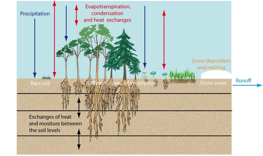
Figure 3.8: The main processes that have to be taken into account in a land
surface model. For clarity, the carbon storage in plants and in soils, as well
as the exchanges between these reservoirs and with the atmosphere are not
shown.
Sophisticated representations of these processes are now included in the state-of-
the-art GCMs. In particular, they include a multi-layer soil model, a comprehensive
description of the vegetation cover and of the physical and chemical interactions between
the plants, the soil and the atmosphere. They also have a sophisticated river-routing
scheme which accounts for the duration of the water transport as well as evaporation
during the journey to the ocean or the interior sea. These improvements are also essential
in an adequate representation of the carbon cycle on land (see section 2.3.3). At present,
the majority of climate models do not include a representation of permafrost, but this is
likely to change because of the large modifications in the extent of permafrost that are
expected during the 21st century.
Some models take the community composition and vegetation structure as a
boundary condition or forcing (if land use changes are specified for instance). They then
use this information to determine the physical characteristics of the surface and the soil,
as well as the carbon storage over land. However dynamic global vegetation models
(DGVMs) explicitly compute the transient dynamics of the vegetation cover in response
to climate changes and disturbances such as fires. DGVMs can also provide the
distribution of biomes that are in equilibrium with climate conditions (Figure 3.9). It is of
course impossible to represent the fraction covered by each of the hundreds of thousands
of different plant species in DGVMs. The plants are thus grouped into plant functional
types (PFTs) that share common characteristics. Very simple models only use two PFTs
(trees and grass, the area not covered by trees or grass corresponding to the fraction of
desert in a grid element), while more sophisticated models use more than ten different
PFTs.
71Goosse H., P.Y. Barriat, W. Lefebvre, M.F. Loutre and V. Zunz (2010)
Figure 3.9: The equilibrium fraction of trees in a model that includes two plant
functional types and whose community composition is only influenced by
precipitation and the growing degree days (GDD) (Brovkin et al. 1997). Growing
degree days are defined as the sum of the daily mean near-surface temperatures for
the days of a year with a temperature higher than 0°C. Figure Courtesy of V.
Brovkin.
3.3.5 Marine biogeochemistry
Models of biogeochemical cycles in the oceans are based on a set of equations
whose formulation is very close to that of equations 3.10 and 3.11 for the ocean
temperature and salinity:
dTracbgc
= Fdiff + Sources − Sinks (3.16)
dt
where Tracbgc is a biogeochemical variable. Those variables are often called tracers
because they are transported and diffused by the oceanic flow (the left hand side of the
equation and the term Fdiff).
723. Modelling of the climate system
Tracbgc can represent DIC, Alk, the concentration of various chemical species
(including nutriments necessary for phytoplankton growth) or the biomass of different
groups of phytoplankton, detritus, zooplankton and (more rarely) higher trophic levels.
Simplified carbon cycle models include a few state variables while the most sophisticated
biogeochemical models have more than 30 of them. The Sources and Sinks terms account
for the increase or decrease of the tracer concentration in response to biogeochemical
processes, including thus a representation of the processes described in section 2.3. For
instance, for a particular phytoplankton group, the Sources term could be related to the
growth in the biomass by photosynthesis, while the Sinks are the consumption of
phytoplankton by zooplankton as well as the mortality of the cells. In addition to the
processes taking place in the water column, some models include a comprehensive ocean
sediment component in order to be able to study the long-term changes in the carbon
cycle.
Figure 3.10: A simplified scheme representing some of the variables of a
biogeochemical model. The interactions between the groups are complex as
the different types of phytoplankton need different nutrients, are grazed by
different types of zooplankton etc.
3.3.6 Ice sheets
As already discussed for the atmosphere and the sea ice, ice-sheet models can be
decomposed into two major components: a dynamic core that computes the flow of the
ice and a thermodynamic part that estimates the changes in ice temperatures, snow
accumulation, melting, etc. The ice velocity can be computed using the complete three-
73Goosse H., P.Y. Barriat, W. Lefebvre, M.F. Loutre and V. Zunz (2010)
dimensional equation. This is affordable for regional models, focusing on particular
regions, but approximations are often necessary for climate models which compute the
development of whole ice sheets on long timescales.
The conservation of ice volume can be written as:
∂H G G
= −∇.(v mH ) + Mb (3.17)
∂t
G
where v m is the depth-averaged horizontal velocity field and Mb is the mass balance
accounting for snow accumulation as well as basal and surface meltings. Surface melting
can be deduced from the energy budget at the surface (similar to Eq. 2.36, see also
section 3.3.3). Simpler formulations of surface melting are based on the positive degree-
day methods, which relates the melting to the temperature during the days with
temperatures above 0°C. An important element in the mass balance at the surface of the
ice sheets is the position of the equilibrium line between the regions where, on a yearly
average, snow tends to accumulate and the ablation region (where there is net melting of
the snow and ice when the surface mass balance is integrated over the whole year). On
the Greenland ice sheet, in present-day conditions, ablation occurs in many areas,
whereas on the colder Antarctic ice sheet, it is restricted to a few regions only.
Figure 3.11: The main processes that have to be taken into account in an ice
sheet model. Figure reproduced from
http://www.solcomhouse.com/icecap.htm.
The melting at the ice base is deduced from the balance between the heat
conduction in the ice and in the ground, taking into account the geothermal heat flux.
Conditions at the ice base, and in particular the presence of water or ice close to the
melting point at the corresponding pressure, have a large impact on the ice velocity as
they reduce the stresses greatly, compared to the situation where the ice is well below the
freezing point.
743. Modelling of the climate system
Ice sheets models also need to take into account the interactions between grounded
ice and ice shelves. Because of local melting and iceberg calving, ice shelves can make a
large contribution to the mass balance of the ice sheets, as is currently the case for
Antarctica. Furthermore, they generate stresses that tend to slow down the ice flow on
land. Indeed, observations have shown that the recent breakdown of some ice shelves has
produced, in some regions, an acceleration of the land ice.
An additional element in ice-sheet models is the representation of interactions with
the underlying bedrock. In particular, as the load of the ice sheet tends to depress the
bedrock, a bedrock adjustment model is needed to compute the position of the ground as
a function of the ice mass. This then yields the elevation of the ice sheet as a function of
the ice thickness.
3.3.7 Coupling between the components - Earth system models
The interactions between the various components of the system play a crucial role
in the dynamics of climate. Wind stress, heat and freshwater fluxes at the ocean surface
are the main drivers of the ocean circulation (see section 1.3.2). The evaporation at the
ocean surface is the largest source of water vapour for the atmosphere, which influences
the radiative properties of the air (section 2.1.2) and the atmospheric heat transport
(section 2.1.5). Snow falling on ice sheets is an essential element of their mass balance.
Many other examples could be cited.
Some of those interactions are quite straightforward to compute from the models
state variables, while more sophisticated parameterisations are required for others. For
instance, the parameterisation of the wind stress and of the heat flux at the atmospheric
base (e.g., Eqs. 2.33 and 2.34) can be derived from theories of the atmospheric
boundary layer. However, this computation still requires empirical parameters that
depend on the characteristics of the surface, introducing some uncertainties into the
determination of the flux.
The technical coupling of the various components to obtain a climate- or Earth-
system model brings additional difficulties. The numerical codes have generally been
developed independently by different groups, using different coding standards, different
numerical grids, etc. It is thus necessary to design an interface and to use a coupler, i.e.
code specially adapted to represent the exchanges between the various components.
The above presentation includes the main elements of the majority of current Earth-
system models. However, the description is far from exhaustive. New components (such
as models of the methane cycle, of the nitrogen cycle, more sophisticated representation
of atmospheric chemistry, etc) are continuously included in order to obtain a more
comprehensive representation of the complex interactions in the system.
3.4 Numerical resolution of the equations
3.4.1 Consistence, convergence and stability
The equations that rule the climate system are partial differential equations
(PDEs) such as those presented in section 3.3, except when extremely simplified models
are used (section 3.2.1). It is first necessary to ensure that those equations are
mathematically well-posed, i.e. that the problem has a unique solution that depends on
the initial and boundary conditions. This requires that those initial and boundary
conditions are properly specified. For instance, to solve the equation for temperature in
the ocean knowing the velocity field (Eq. 3.10), we must specify the initial temperature
75Goosse H., P.Y. Barriat, W. Lefebvre, M.F. Loutre and V. Zunz (2010)
over the whole domain at a time t0 as well as one boundary condition over all the points
of the spatial boundaries of the domain, which can be the value of the heat flux or of the
temperature there. Below, we will consider that all the problems investigated are well-
posed.
In order to solve the equations of the mathematical models developed for each
component of the climate system (section 3.3), those models have to be transformed into
numerical models that can be handled by a computer. The first method, which is probably
the easiest to understand, is to approximate the derivatives in the partial differential
equations by finite differences. This is called the finite difference method. The solution
is no longer a continuous function (as for the PDEs) but a discrete one, only defined for
specific times separated by the time step Δt, and specific locations separated by the
spatial step Δx (plus Δy and Δz for a problem with three spatial dimensions).
Imagine for instance, a very simple ordinary differential equation:
du
= A cos(t ) (3.18)
dt
where t is the time, u a state variable (for instance the velocity) which depends here only
on the time, and A a constant. The derivative according to time could be approximated by
a finite difference, leading to the finite difference equation:
U n +1 − U n
= A cos(nΔt ) (3.19)
Δt
Un is the discrete solution of the finite difference equation at time step n. If Δt is constant,
t=n Δt, assuming that the initial time is 0.
Figure 3.12: The analytical solution of equation 3.18 using A=1 and u(t=0)=0
(black) and the numerical solution using Eq. 3.20 with a time step Δt =π/50 (red).
The discrete solution Un at times nΔt have been joined by straight lines. Note that a
much more precise solution could be obtained by using
U = U + Δt ( A cos(( n + 1/ 2)Δt ) ) instead of Eq.3.20, i.e. by evaluating the
n +1 n
cosine at time t=(t+1/2)Δt instead of time t=nΔt.
763. Modelling of the climate system
Knowing Un, this equation can be easily solved for Un+1(Fig. 3.12):
U n +1 = U n + Δt ( A cos(nΔt )) (3.20)
Such problems are called initial value problems because, when the initial value is
specified, values for any time can be obtained by advancing or “marching” in time.
For a numerical method to be adequate, two fundamental properties must hold.
First, the finite difference equation must be consistent with the partial differential
equation. This means that as Δt → 0, Δx → 0 , the finite differential equation coincides
with the PDE. This is absolutely essential to ensure that the equation that has been solved
numerically is a reasonable approximation to the mathematical model. It can be checked
by replacing all the terms by the Taylor series expansion. For the left-hand side of
Equation 3.19, this gives:
du 1 d 2u 2
U n +1 = U n + Δt + Δt + higher order terms (3.21)
dt 2 dt 2
and thus
U n +1 − U n du 1 d 2u
= + Δt + higher order terms (3.22)
Δt dt 2 dt 2
which effectively tends to du/dt as Δt tends to 0. This shows that the scheme is consistent.
Secondly, the solution of the finite difference must converge to the solution of the
PDE as Δt → 0, Δx → 0 . In our example, this means that
U (nΔt ) → u(t ) when Δt → 0 (3.23)
This convergence is related to the computational stability which states that a
numerical scheme is computationally stable if the solution of the finite difference
equation at a fixed time remains bounded as Δt → 0 . In more colourful language, it can
be said that, in this case, the numerical model does not explode. Indeed, the Lax-
Richtmyer theorem, which can be formally demonstrated for a well-posed initial-value
problem, states that, for a consistent numerical method, stability and convergence are
equivalent.
As a consequence, the practical methods used to test the convergence of a
numerical scheme are based on an analysis of the stability of the scheme. In some cases,
it is possible to explicitly demonstrate that the solution is bounded, a propriety generally
conditioned by a criteria that governs Δt and Δx. A more general criterion to determine
the largest time and spatial step allowed is the von Neumann method in which the
stability of the finite difference equation is analysed by expressing the solution as an
expansion of an appropriate set of basis functions, generally Fourier series.
Analyses such as the one performed in Equation 3.22 also allow a truncation error
(i.e. the difference between the PDE and the finite difference equation) to be defined.
This error is characterised by an order, corresponding to the power of the first term of the
difference. For the scheme described above, the error is thus of the first order in time. In
77Goosse H., P.Y. Barriat, W. Lefebvre, M.F. Loutre and V. Zunz (2010)
addition to uncertainties relating to the physical model itself, and the definition of initial
and boundary conditions, the representation of numbers by computers using a finite
number of digits is also a source of error in the numerical solution.
3.4.2 Time and space discretisations using finite differences
Many options are available for discretising an equation and the choice depends on
the properties required in the numerical scheme. In addition to consistency and the
stability for reasonably long time steps, the scheme must be precise enough, but not too
demanding of computer time. We have presented a first example of time discretisation in
section 3.4.1, which is called the upward scheme (or forward Euler method):
U n +1 − U n
= F (U n ) (3.24)
Δt
for a right-hand side represented in a general way as a function F(Un).
An alternative scheme is a centred difference (leapfrog scheme):
U n +1 − U n −1
= F (U n ) (3.25)
2Δt
which has a second order truncation error and is thus in principle more precise than the
first order upward scheme. However, this scheme allows the presence and growth of
unphysical modes, and is thus generally stabilised by associating it with a time filter.
In implicit schemes, the right-hand side is not only expressed at time step n but also
at time step n+1. F then becomes, in general, a function of both Un and Un+1. If F is only
a function of Un+1, the scheme is called fully implicit or backward. Implicit schemes
require an equation or a system of equations to be solved to obtain Un+1, equations that
could be non-linear. Implicit schemes could thus be relatively expensive in computer
time. On the other hand, implicit schemes allow longer time steps, which in some
circumstances is a clear advantage.
The same variety of numerical schemes is available for space discretisation.
Consider the diffusion equation:
∂u ∂ 2u
=k 2 (3.26)
∂t ∂x
where k is a constant. This can be discretised as:
U nj +1 − U nj U nj +1 − 2U nj + U nj −1
=k (3.27)
Δt Δx 2
The index j refers to point number j of the spatial grid, which is at a distance (j-1)Δx from
the first grid point if the grid spacing Δx is constant. It can easily be shown that this
scheme is consistent and that the truncation error is first order in time and second order in
space. It is stable if:
783. Modelling of the climate system
Δt 1
k ≤ (3.28)
Δx 2
2
illustrating the link usually present between Δt and Δx. Using this scheme, the solution at
point j is updated at each time step n+1 from the values computed at time step n for
points j-1, j and j+1 (Fig. 3.13).
Figure 3.13: Schematic representation of the grid structure in space and time with
one spatial dimension for the numerical scheme proposed in Eq. 3.27, showing that
U nj +1 dependents on U nj −1 , U nj , U nj+1 ..
In the two examples above (Eqs. 3.18 and 3.26), only one equation for one variable
was solved. However, when all the components of the climate system are considered,
equations for several variables must be solved simultaneously. For numerical reasons,
those variables are not necessary located at the same place on the grid, leading to what
are called staggered grids. Arakawa and Lamb (1977) proposed a classification of these
grids. Two popular ones are the B and the C grid. If we consider an elementary square of
the grid for an ocean model, for instance, for the B grid, the temperature T (as well as the
salinity, the pressure, and the density) are computed at the centres of the grid while the
velocity components u and v are obtained at the corners of the grid elements (Figure
3.14). For the C grid, the velocities are computed on the side of the elements. Staggered
grids are also widely used for vertical elements, with the velocity usually computed at the
boundary between the layers, while the temperature is defined at the centre of the layers.
79Goosse H., P.Y. Barriat, W. Lefebvre, M.F. Loutre and V. Zunz (2010)
Figure 3.14: The location of some variables on the staggered grids B and C
according to Arakawa and Lamb’s (1977) classification.
3.4.3 Spectral representation and finite element methods
In addition to finite differences, several other methods can be use to discretise
equations. One method is to integrate the basic equation of the system over a finite
volume before the discretisation. This finite-volume method, has the advantage that it
explicitly and easily ensures the conservation of some important properties. If particular
hypotheses are made about the changes in the variables inside the volumes, numerical
schemes similar to those described using finite-difference methods can be obtained.
In the Galerkin approach, the numerical solution is discretised in space as a sum of
k basis functions ϕk(x) using coefficients Ak that depend on the time, leading to a spectral
representation of the solution:
K
U ( x, t ) = ∑ Ak (t )ϕk ( x ) (3.29)
k =1
The goal of the resolution of the problem is then to determine the coefficients Ak. The
larger the number of basis functions retained (i.e. the larger k is), the more precise is the
spatial representation of the solution. The big advantage of this method is that the space
derivation of U(x,t) can be analytically computed from dϕk(x)/dx without any additional
approximation. The choice of the basis function must be adequate. For a one-dimensional
problem, Fourier series are a natural choice. For a problem with spherical geometry, in
particular for global atmospheric models, spherical harmonics are used. They are the
product of Fourier series in longitude and associated Legendre polynomials in latitude.
The spectral and grid-point (also referred to as physical space, see for instance Fig.
3.13) representations are complementary. The first provides an accurate computation of
horizontal derivatives while the second forms a convenient framework to evaluate non-
linear terms as well as the physics of the model (for example, the computation of the
radiative transfer). When the two approaches are combined, some transfers of the
variables from the physical to the spectral space are required in the transform method.
There must be an exact correspondence between the number of basis function and the
horizontal resolution of the grid to avoid numerical problems during this transformation.
The finite element approach is based on a similar approximation to Eq. 3.29 but
instead of functions ϕk(x) that cover the whole domain as in the spectral method, local
basis functions are used. For example, ϕk(x) can be a piecewise linear function equal to 1
at a grid point and 0 at all the other points.
803. Modelling of the climate system
3.5 Testing the validity of models
3.5.1 Verification, validation, testing
Despite very careful design, there is no guarantee that a computer model will be
adequate for its intended use: some processes treated as negligible can turn out to be more
important than initially thought; a parameterisation may not be valid in the particular
conditions of interest or may be incompatible with other hypotheses employed; the
selection of parameters can be far from optimal; and so on. As a consequence, climate
models have to be tested to assess their quality and evaluate their performance. In this
framework, it is always necessary to keep in mind the scientific objectives of the study
(or studies) that will be conducted using a particular model. Although the principles
remain the same, the tests performed with a model developed to analysing the
development of the global carbon cycle over the last million years (see section 5.3.2) are
clearly different from those for a model providing projections of future climate changes at
the highest possible resolution (see Chapter 6).
A first step is to ensure that the numerical model solves the equations of the
physical model adequately. This procedure, often referred to as verification (Fig. 3.15),
only deals with the numerical resolution of the equations in the model, not with the
agreement between the model and reality. It checks that no coding errors have been
introduced into the program. The numerical methods used to solve the model equations
must also be sufficiently accurate. Different methods are available to achieve this goal. A
standard one is to compare the numerical solution with the analytical one for highly
idealised test cases for which an exact solution is available. It is also possible to formally
state that some parts of the code are correct, for instance, the one that solves large
systems of n linear algebraic equations with n unknowns (which are often produced as
part of the numerical resolution of the partial differential equations on the model grid).
Figure 3.15: A modified version of Fig. 3.1 illustrating the verification and
validation processes. An additional arrow from the analysis of the results towards
model development has been added to show that validation is a continuous
process.
81Goosse H., P.Y. Barriat, W. Lefebvre, M.F. Loutre and V. Zunz (2010)
The next step is the validation process, i.e. determining whether the model
accurately represents reality. To do this, the model results have to be compared with
observations obtained in the same conditions. In particular, this implies that the boundary
conditions and forcings must be correctly specified to represent the observed situation.
Validation must first be performed on the representation of individual physical
processes, such as the formulation of the changes in the snow albedo in response to
surface melting and temperature change. This is generally achieved for particular
locations, during field campaigns specifically designed to study this process. They
provide a much larger amount of very specific data than global data bases, allowing a
detailed evaluation of the performance of the model on this topic. On a larger scale, the
different components of the model (atmosphere, ocean, sea ice, etc, see section 3.3) have
to be tested independently, ensuring that the boundary conditions at the interface with the
other components are well defined. Finally, the results of the whole coupled model have
to be compared with observations. All those steps are necessary because bad surprises are
always possible after the different elements are coupled together, due to non-linear
interactions between the components. Some problems with the model can also be masked
by the formulation of the boundary conditions when components are run individually.
However, having a coupled model providing reasonable results is not enough. In order to
test whether the results occur for the correct reason, it is necessary to check that all the
elements of the model are doing a good job, and that the satisfactory overall behaviour of
the model is not due to several errors in its various elements cancelling each other out.
When discussing verification and validation, we must always recognize that both
of them can only be partial for a climate model, except maybe in some trivial cases. The
accuracy of the numerical solution can only be estimated for small elements of the code
or in very special (simplified) conditions. Indeed, if it were possible to obtain a very
accurate solution to compare with the numerical model results in all possible cases, there
would be no point in developing a numerical model! The comparison of model results
with observations is also limited to some particular conditions and completely validating
a climate model in all the potential situations would require an infinite number of tests. A
climate model could thus never be considered as formally verified or validated. A model
is sometimes said to be validated if it has passed a reasonable number of tests. In such a
case, the credibility of model projections performed with such a model could be very
high. However, there is no way to formally guarantee that the results of the model will be
correct even if the conditions are only slightly different from those used in the validation
process, in particular for a very complex system like the climate. Furthermore, there is no
agreement in climatology as to what a reasonable number of tests is.
The term “a validated model” and phrases like “the model has been validated” must
therefore be avoided. Rather, the verification and validation should be considered as
processes that never lead to a final, definitive product. The model should be continuously
re-tested as new data or experimental results become available. The building of a model
could then be viewed in the same way as a scientific theory. Hypotheses are formulated
and a first version of the model developed. The results of the model are then compared to
observations. If the model results are in good agreement with the data, the model could be
said as to be confirmed for those conditions, so increasing its credibility. Nevertheless,
this does not mean that the model is validated for all possible cases. If the model results
do not compare well with observations, the model should be improved. This could lead to
new hypotheses, to additional terms in the governing equations, or to the inclusion of new
processes by new equations or new parameterisations.
Alternatively, a disagreement between the model and observations can be related to
an inadequate selection of the values of some parameters that are not precisely known
(for instance the exchange coefficients in Eqs. 2.33 and 2.34). Adjusting those parameters
is part of the calibration of the model, also referred to as tuning. Model developers and
823. Modelling of the climate system
users also may decide that, if the model cannot reproduce the observations in some
special cases, this indicates that it is not valid for such conditions, although it can still be
used in other situations where the tests indicate better behaviour. For instance, we can
imagine a climate model that cannot simulate the climate of Mars correctly without some
modifications; however, this does not invalidate it for modelling conditions on Earth. On
the other hand, if it works well for both Mars and Earth, this is a good test of its
robustness.
The calibration of physical parameters is generally required and is perfectly
justified as there is no a priori reason to select one particular value in the observed range
of the parameters. It is also valid to calibrate the numerical parameters in order to obtain
the most accurate numerical solution of the equations. However, care has to be taken to
ensure that the calibration is not a way of artificially masking some deficiencies in the
model. If this does occur, there is a high probability that the selected parameters will not
provide satisfactory results for other conditions (e.g. the climate at the end of the 21st
century). Performing many tests for widely different situations and for various elements
of the model should limit the risk, but the number of observations is often too small to
ensure that the problem has been completely avoided. An additional problem with the
constant improvement of the model and of its calibration as soon as new data becomes
available is the absence of independent data to really test the performance of the model.
Ideally, some of the available information should be used for the model development and
calibration, and some should be kept to assess its accuracy. Another good model practise
is to choose or design models components for which the selection of one particular value
of the parameters has only a small impact on model results, so reducing importance of the
calibration.
In all the tests performed with the model, it is necessary to estimate the agreement
between model results and observations. This is a complex and sometimes under-valued
task. Indeed, the comparisons between the results of various models have shown that a
single model is never the best for all the regions and variables analysed. Introducing a
new parameterisation or changing the value of a parameter usually improves the results in
some areas and worsens them in others. The agreement should then be related to the
intended use of the model. This could be done more or less intuitively by visually
comparing maps or plots describing both the model results and the observations.
However, a much better solution is to define an appropriate metric. For a single field,
such as the annual mean surface temperature Ts, a simple root mean square (RMS) error
may be appropriate:
1 n k
RMS = ∑
n k =1
(Ts,mod −Tsk,obs )2 (3.30)
where n is the number of grid points for which observations are available, Tsk,mod is the
model surface temperature at point k and Tsk,obs is the observed surface temperature at
point k. This estimate could be improved by taking into account the area of each grid
point or by giving greater weight to the regions of most interest. If many variables have to
be included in the metric, the RMS errors of different variables can be combined in
various ways. The model data-comparison should also take into account the errors or
uncertainties in both the model results and the observations. Errors in the observations
can be directly related to the precision of the instruments or of the indirect method used
to retrieve the climate signal (see for instance section 5.3.3). The uncertainties could also
be due to the internal variability of the system (see sections 1.1 and 5.2), because
83You can also read