Machine dependence and reproducibility for coupled climate simulations: the HadGEM3-GC3.1 CMIP Preindustrial simulation - Geosci. Model Dev.
←
→
Page content transcription
If your browser does not render page correctly, please read the page content below
Geosci. Model Dev., 13, 139–154, 2020
https://doi.org/10.5194/gmd-13-139-2020
© Author(s) 2020. This work is distributed under
the Creative Commons Attribution 4.0 License.

Machine dependence and reproducibility for coupled climate
simulations: the HadGEM3-GC3.1 CMIP Preindustrial simulation
Maria-Vittoria Guarino1 , Louise C. Sime1 , David Schroeder2 , Grenville M. S. Lister3 , and Rosalyn Hatcher3
1 BritishAntarctic Survey, Cambridge, UK
2 Department of Meteorology, University of Reading, Reading, UK
3 National Centre for Atmospheric Science, University of Reading, Reading, UK

Correspondence: Maria-Vittoria Guarino (m.v.guarino@bas.ac.uk)

Received: 28 March 2019 – Discussion started: 16 May 2019
Revised: 29 November 2019 – Accepted: 4 December 2019 – Published: 16 January 2020

Abstract. When the same weather or climate simulation is          1   Introduction
run on different high-performance computing (HPC) plat-
forms, model outputs may not be identical for a given ini-        The UK CMIP6 (Coupled Model Intercomparison Project
tial condition. While the role of HPC platforms in delivering     Phase 6) community runs individual MIP (Model Intercom-
better climate projections is to some extent discussed in the     parison Project) experiments on differing computing plat-
literature, attention is mainly focused on scalability and per-   forms but will generally compare results against the refer-
formance rather than on the impact of machine-dependent           ence simulations run on the UK Met Office platform. For
processes on the numerical solution.                              this reason, within the UK CMIP community, the possible
   Here we investigate the behaviour of the Preindustrial (PI)    influence of machine dependence on simulation results is of-
simulation prepared by the UK Met Office for the forth-           ten informally discussed among scientists, but surprisingly
coming CMIP6 (Coupled Model Intercomparison Project               an analysis to quantify its impact has not been attempted.
Phase 6) under different computing environments.                     The issue of being able to reproduce identical simula-
   Discrepancies between the means of key climate variables       tion results across different supercomputers, or following
were analysed at different timescales, from decadal to cen-       a system upgrade on the same supercomputer, has long
tennial. We found that for the two simulations to be statis-      been known by numerical modellers and computer scientists.
tically indistinguishable, a 200-year averaging period must       However, the impact that a different computing environment
be used for the analysis of the results. Thus, constant-forcing   can have on otherwise identical numerical simulations ap-
climate simulations using the HadGEM3-GC3.1 model are             pears to be little known by climate model users and model
reproducible on different HPC platforms provided that a suf-      data analysts. In fact, the subject is rarely ever addressed in
ficiently long duration of simulation is used.                    a way that helps the community understand the magnitude
   In regions where El Niño–Southern Oscillation (ENSO)           of the problem or to develop practical guidelines that take
teleconnection patterns were detected, we found large             account of the issue.
sea surface temperature and sea ice concentration differ-            To the extent of our knowledge, only a few authors have
ences on centennial timescales. This indicates that a 100-        discussed the existence of machine dependence uncertainty
year constant-forcing climate simulation may not be long          and highlighted the importance of bit-for-bit numerical re-
enough to adequately capture the internal variability of the      producibility in the context of climate model simulations.
HadGEM3-GC3.1 model, despite this being the minimum               Song et al. (2012) and Hong et al. (2013) investigated the
simulation length recommended by CMIP6 protocols for              uncertainty due to the round-off error in climate simulations.
many MIP (Model Intercomparison Project) experiments.             Liu et al. (2015a, b) discussed the importance of bitwise iden-
   On the basis of our findings, we recommend a minimum           tical reproducibility in climate models.
simulation length of 200 years whenever possible.                    In this paper, we investigate the behaviour of the
                                                                  UK CMIP6 Preindustrial (PI) control simulation with the

Published by Copernicus Publications on behalf of the European Geosciences Union.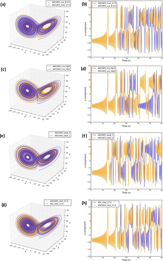
140 M.-V. Guarino et al.: Machine dependence and reproducibility for coupled climate simulations
HadGEM3-GC3.1 model on two different high-performance tialized with (x0 , y0 , z0 ) ≡ (1, 1, 1) and numerically inte-
computing (HPC) platforms. We first study whether the two grated with a 4th-order Runge–Kutta scheme using a time
versions of the PI simulation show significant differences in step of 0.01. The Lorenz model was run on two HPC plat-
their long-term statistics. This answers our first question of forms, namely the UK Met Office Supercomputer (here-
whether the HadGEM3-GC3.1 model gives different results inafter simply “MO”) and ARCHER.
on different HPC platforms. To first demonstrate the implications of switching between
Machine-dependent processes can influence the model in- different computing environments, the Lorenz model was run
ternal variability by causing it to be sampled differently on on the ARCHER platform using the following:
the two platforms (i.e. similarly to what happens to en-
– two different FORTRAN compilers (cce8.5.8 and in-
semble members initiated from different initial conditions).
tel17.0; see Fig. 1a and b);
Therefore, our second objective is to quantify discrepancies
between the two simulations at different timescales (from – same FORTRAN compiler (cce8.5.8) but different
decadal to centennial) in order to identify an averaging pe- degrees of floating-point optimization (-hfp0 and
riod and/or simulation length for which the two simulations -hfp3; see Fig. 1c and d); and
return the same internal variability.
– the same FORTRAN (cce8.5.8) compiler and compil-
Note that the PI control simulation is a constant-forcing
ing options, but the x component in Eqs. (1)–(3) was
simulation. Therefore, no ensemble members are required for
perturbed by adding a noise term obtained using the
such an experiment because, provided that the simulation is
random_number and random_seed intrinsic FOR-
long enough, it will return a picture of the natural climate
TRAN functions. In particular, the seed of the random
variability.
number generator was set to 1 and 3 in two separate ex-
The remainder of the paper is organized as follows. In
periments; see Fig. 1e and f.
Sect. 2, mechanisms by which the computing environment
can influence the numerical solution of chaotic dynamical Finally, to illustrate the role of using different HPC plat-
systems are reviewed and discussed. In Sect. 3, the numerical forms, the Lorenz model was run on the ARCHER and MO
simulations are presented, and the methodology used for the platforms using the same compiler (intel17.0) and identical
data analysis is described. In Sect. 4, the simulation results compiling options (i.e. level of code optimization, floating-
are presented and discussed. In Sect. 5, the main conclusions point precision, vectorization) (Fig. 1g and h).
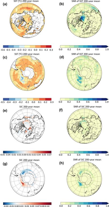
of the present study are summarized. The divergence of the solutions in Fig. 1a and b can likely
be explained by the different “computation order” of the two
compilers (i.e. the order in which the same arithmetic expres-
2 The impact of machine dependence on the numerical sion is computed). In Fig. 1c and d, solutions differ because
solution of the round-off error introduced by the different precision
of floating-point computation. In Fig. 1e and f, the different
In this section, possible known ways in which machine-
seed used to generate random numbers caused the system to
dependent processes can influence the numerical solution of
be perturbed differently in the two cases. While this conclu-
chaotic dynamical systems are reviewed and discussed.
sion is straightforward, it is worth mentioning that the use
Different compiling options, degrees of code optimization,
of random numbers is widespread in weather and climate
and basic library functions all have the potential to affect the
modelling. Random number generators are largely used in
reproducibility of model results across different HPC plat-
physics parameterizations for initialization and perturbation
forms and on the same platform under different computing
purposes (e.g. clouds, radiation, and turbulence parameteri-
environments. Here we provide a few examples of machine-
zations) as well as in stochastic parameterizations. The pro-
dependent numerical solutions using the 3-D Lorenz model
cesses by which initial seeds are selected within the model
(Lorenz, 1963), which is a simplified model for convection
code are thus crucial in order to ensure numerical repro-
in deterministic flows. The Lorenz model consists of the fol-
ducibility. Furthermore, different compilers may have differ-
lowing three differential equations:
ent default seeds.
dx As for Fig. 1g and h, this is probably the most relevant
= α(y − x), (1) result for the present paper. It highlights the influence of the
dt
dy HPC platform (and of its hardware specifications) on the final
= γ x − y − zx, (2) numerical solution. In Fig. 1g and h the two solutions diverge
dt
dz in time similarly to Fig. 1a–d; however, identifying reasons
= xy − βz, (3) for the observed differences is not straightforward. While we
dt
speculate that reasons may be down to the machine archi-
where the parameters α = 10, γ = 28, and β = 8/3 were tecture and/or chip set, further investigations on the subject
chosen to allow for the generation of flow instabilities and were not pursued as this would be beyond the scope of this
obtain chaotic solutions (Lorenz, 1963). The model was ini- study.
Geosci. Model Dev., 13, 139–154, 2020 www.geosci-model-dev.net/13/139/2020/
M.-V. Guarino et al.: Machine dependence and reproducibility for coupled climate simulations                                           141

Figure 1. Attractor (left-hand side) and time series of the x component (right-hand side) of the 3-D Lorenz model for simulations run on
ARCHER using the cce8.5.8 and intel17.0 compilers (a, b), the same compiler (cce8.5.8) but a different level of floating-point optimization
(hfp0, hfp3) (c, d), and the same compiler (cce8.5.8) and compiling options but a different seed for the random number generator (seed 1, 3)
(e, f). Panels (g) and (h) are the Lorenz attractor and the x component time series for the Lorenz model run on MO and ARCHER using the
same compiler (intel17.0) and compiling options.

www.geosci-model-dev.net/13/139/2020/                                                          Geosci. Model Dev., 13, 139–154, 2020
142                       M.-V. Guarino et al.: Machine dependence and reproducibility for coupled climate simulations

   The three mechanisms discussed above were selected be-         Table 1. Hardware and software specifications of the ARCHER and
cause they are illustrative of the problem and easily testable    MO HPC platforms as used to run the HadGEM3-GC3.1 model.
via a simple model such as the Lorenz model. However, there
are a number of additional software and hardware specifica-            HPC platform     Machine      Compiler    Processor
tions that can influence numerical reproducibility and that            MO               Cray XC40    cce 8.3.4   Broadwell
only emerge when more complex codes, like weather and                  ARCHER           Cray XC30    cce 8.5.8   Ivy Bridge
climate models, are run. These are the number of processors
and processor decomposition, communications software (i.e.
MPI libraries), and threading (i.e. OpenMP libraries).
                                                                  on the MO HPC platform on 2500 cores. The model was
   We conclude this section by stressing that the four case
                                                                  at first run for 700 model years to allow the atmospheric
studies presented in Fig. 1 (and the additional mechanisms
                                                                  and oceanic masses to attain a steady state (model spin-
discussed in this section) are all essentially a consequence of
                                                                  up) and then run for a further 500 model years (actual run
the chaotic nature of the system. When machine-dependent
                                                                  length) (see Menary et al., 2018 for details). A copy of the
processes introduce a small perturbation or error into the sys-
                                                                  PI control simulation was ported to the ARCHER HPC plat-
tem (no matter by which means), they cause it to evolve dif-
                                                                  form (hereinafter referred to as PIAR ), initialized using the
ferently after a few time steps.
                                                                  atmospheric and oceanic fields from the end of the spin-
                                                                  up, and run for 200 model years using 1500 cores. The
                                                                  source codes of the atmosphere and ocean models were
3     Methodology                                                 compiled on the two platforms using the same levels of
                                                                  code optimization (-O option), vectorization (-Ovector
3.1    Numerical simulations                                      option), and floating-point precision (-hfp option) and, for
                                                                  numerical reproducibility purposes, selecting the least tol-
In this study, we consider two versions of the Preindustrial
                                                                  erant behaviour in terms of code optimization when the
(PI) control simulation prepared by the UK Met Office for
                                                                  number of ranks or threads varies (-hflex_mp option).
the Sixth Coupled Model Intercomparison Project, CMIP6
                                                                  For the atmosphere component the following options were
(Eyring et al., 2016). This PI control experiment is used to
                                                                  used: -O2 -Ovector1 -hfp0 -hflex_mp=strict.
study the (natural) unforced variability of the climate system,
                                                                  For the ocean component the following options were used:
and it is one of the reference simulations against which many
                                                                  -O3 -Ovector1 -hfp0 -hflex_mp=strict.
of the other CMIP6 experiments will be analysed.
                                                                     Table 1 provides an overview of the hardware and software
   The PI simulation considered in this paper uses the
                                                                  specifications of the two HPC platforms on which the model
N96 resolution version of the HadGEM3-GC3.1 climate
                                                                  was run.
model (N96ORCA1). The model set-up, initialization, per-
                                                                     Of the possible mechanisms discussed in Sect. 2, the
formance, and physical basis are documented in Menary
                                                                  ARCHER and MO simulations were likely affected by differ-
et al. (2018) and Williams et al. (2018), to which the
                                                                  ences in compiler, processor type, number of processors, and
reader is referred for a detailed description. In summary,
                                                                  processor decomposition (alongside the different machine).
HadGEM3-GC3.1 is a global coupled atmosphere–land–
                                                                     Note that the porting of the HadGEM3-GC3.1 model from
ocean–ice model that comprises the Unified Model (UM) at-
                                                                  the Met Office computing platform to the ARCHER plat-
mosphere model (Walters et al., 2017), the JULES land sur-
                                                                  form was tested by running 50 ensemble members (each 24 h
face model (Walters et al., 2017), the NEMO ocean model
                                                                  long) on both platforms (this was done by the UK Met Office
(Madec and the NEMO Team, 2015), and the CICE sea ice
                                                                  and NCAS-CMS teams). Each ensemble member was cre-
model (Ridley et al., 2018b). The UM vertical grid contains
                                                                  ated by adding a random bit-level perturbation to a set of se-
85 pressure levels (terrain-following hybrid height coordi-
                                                                  lected variables (x and y components of the wind, air poten-
nates), while the NEMO vertical grid contains 75 depth lev-
                                                                  tial temperature, specific humidity, longwave radiation, etc.).
els (rescaled height coordinates). In the N96 resolution ver-
                                                                  Variables from each set of ensembles were then tested for
sion, the atmospheric model utilizes a horizontal grid spac-
                                                                  significance using a Kolmogorov–Smirnov test to determine
ing of approximately 135 km on a regular latitude–longitude
                                                                  whether they can be assumed to be drawn from the same
grid. The grid spacing of the ocean model, which employs an
                                                                  distribution. These tests did not reveal any significant prob-
orthogonal curvilinear grid, is 1◦ everywhere but decreases
                                                                  lem with the porting of the HadGEM3-GC3.1 model (David
down to 0.33◦ between 15◦ N and 15◦ S of the Equator, as
                                                                  Case, National Centre for Atmospheric Science, University
described by Kuhlbrodt et al. (2018).
                                                                  of Reading, Reading, UK, personal communications, 2019).
   Following the CMIP6 guidelines, the model was initial-
                                                                  However, this method is restricted to timescales shorter than
ized using constant 1850 greenhouse gas (GHG), ozone,
                                                                  1 d. The centennial simulations presented in this paper will
solar, tropospheric aerosol, stratospheric volcanic aerosol,
                                                                  help us understand whether or not differences can arise on
and land use forcings. The UK CMIP6 PI control simu-
                                                                  longer timescales in the HadGEM3-GC3.1 model.
lation (hereinafter referred to as PIMO ) was originally run

Geosci. Model Dev., 13, 139–154, 2020                                                 www.geosci-model-dev.net/13/139/2020/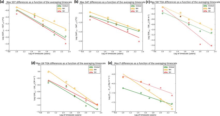
M.-V. Guarino et al.: Machine dependence and reproducibility for coupled climate simulations                                  143

3.2   Data post-processing and analysis                               When SNR < 1, (PIMO − PIAR ) differences can be inter-
                                                                   preted as fluctuations within the estimated range of internal
During the analysis of the results, the following climate vari-    variability. When SNR > 1, (PIMO − PIAR ) differences in the
ables were considered: sea surface temperature (SST), sea ice      mean are outside the expected range of internal variability.
area and sea ice concentration (SIA, SIC), 1.5 m air temper-       This eventuality indicates either a true difference in the mean
ature (SAT), the outgoing longwave and shortwave radiation         or that the expected range of variability is underestimated.
fluxes at top of the atmosphere (LW TOA and SW TOA),                  For the final step of the analysis, the El Niño–Southern
and the precipitation flux (P ). These variables were selected     Oscillation (ENSO) signal was computed for the ARCHER
as representative of the ocean and atmosphere domains and          and MO simulations. We used the Niño 3.4 index, with a 3-
because they are commonly used to evaluate the status of the       month running mean, defined as follows:
climate system.
   Discrepancies between the means of the selected vari-           NINO3.4 = SSTmnth − SST30 yr
ables were analysed at different timescales, from decadal to             if 5 ◦ N ≤ latitude ≤ 5 ◦ S and
centennial. To compute 10-, 30-, 50-, and 100-year means,              120 ◦ W ≤ longitude ≤ 170 ◦ W,                         (5)
(PIMO − PIAR ) 200-year time series were divided into 20,
6, 4, and 2 segments, respectively. Spatial maps were simply       where SSTmnth is the monthly sea surface temperature and
created by averaging each segment over time. Additionally,         SST30 yr is the climatological mean of the first 30 years of
to create the scatter plots presented in Sect. 4.1, the time av-   simulation used to compute the anomalies.
erage was combined with an area-weighted spatial average.
Except for SIC, all the variables were averaged globally. Ad-
                                                                   4     Results and discussion
ditionally, SIC, SST, and SAT were regionally averaged over
the Northern and Southern Hemisphere, while SW TOA, LW             4.1     Multiple timescales
TOA, and P were regionally averaged over the tropics, north-
ern extratropics, and southern extratropics according to the       The long-term means of the selected variables and the associ-
underlying physical processes.                                     ated SNR are shown in Figs. 2 and 3. All the variables exhibit
   Note that, when calculating (PIMO − PIAR ) differences,         SNR < 1, indicating that on multi-centennial timescales the
PIMO and PIAR segments are subtracted in chronological or-         differences observed between the two simulations fall into
der. Thus, for example, the first 10 years of PIAR are sub-        the expected range of variability of the PI control run.
tracted from the first 10 years of PIMO and so on. In fact, be-       When maps like the ones in Figs. 2 and 3 are computed
cause the PI control simulation is run with a constant climate     using 10-, 30-, 50-, and 100-year averaging periods (not
forcing, using a “chronological order” in the strictest sense is   shown), the magnitude of the anomalies increases and (PIMO
meaningless, as every 10-year segment is equally represen-         − PIAR ) differences become significant (SNR  1). This be-
tative of the pre-industrial decadal variability. We acknowl-      haviour is discussed below.
edge that an equally valid alternative approach would be to           Figures 4 to 9 show annual mean time series of spatially
subtract the PIAR and PIMO segments without a prescribed           averaged SST, SIA, SAT, SW TOA, LW TOA, and P , respec-
order.                                                             tively. Figures 4d to 9d show (PIMO − PIAR ) differences as
   Discrepancies in the results between the two runs were          a function of the averaging timescale for each variable (see
quantified by computing the signal-to-noise ratio (SNR) for        Sect. 3.2 for details on the computation of the means). The
each considered variable at each timescale. The signal is          200-year global mean and standard deviation of each variable
represented by the mean of the differences between PIMO            are shown in Table 2.
and PIAR (µMO−AR ), and the noise is represented by the               For all the considered variables, PIMO and PIAR start di-
standard deviation of PIMO (σMO ), our “reference” simula-         verging quickly after the first few time steps once the system
tion. Because of the basic properties of variance, for which       has lost memory of the initial conditions (Figs. 4 to 9, pan-
VarX−Y = VarX +VarY −2Cov(X, Y ) (Loeve, 1977), we can             els a, b, c). See Sect. 2 (Fig. 1) for a further discussion on
more conveniently express the noise as σMO = σMO−AR    √     un-   how machine-dependent processes can influence the tempo-
                                                         2
der the assumption that PIMO and PIAR are uncorrelated             ral evolution of the system.
(Cov(MO, AR) = 0) and have the same variance (VarMO =                 SST, SAT, SW TOA, and LW TOA differ the most
VarAR ). This allowed us to compute SNR on one grid and            in the Northern Hemisphere (and particularly on decadal
avoid divisions by (nearly) zero when the sea ice field be-        timescales) (yellow diamonds in Figs. 4d, 6d, 7d, 8d), while
tween PIMO and PIAR evolved differently, resulting in unre-        SIA anomalies are particularly high in the Southern Hemi-
alistically high SNR values along the sea ice edges. Finally,      sphere (red crosses in Fig. 5d) and P anomalies in the trop-
SNR is defined as                                                  ics (green circles in Fig. 9d). Overall, discrepancies are the
          |µMO−AR | |µMO−AR |                                      largest at decadal timescales at which the spread between the
SNR =                = σ           .                         (4)   two simulations can reach |0.2| ◦ C in global mean air tem-
             σMO           MO−AR
                            √                                      perature (Fig. 6d), |1.2| million km2 in Southern Hemisphere
                              2

www.geosci-model-dev.net/13/139/2020/                                                     Geosci. Model Dev., 13, 139–154, 2020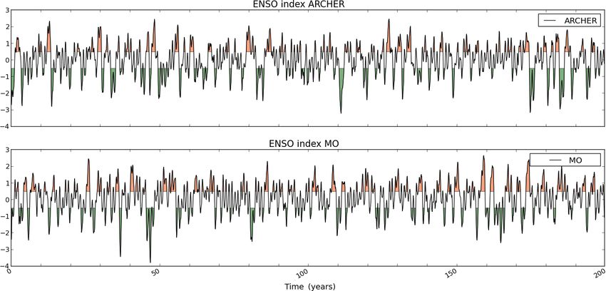
144                       M.-V. Guarino et al.: Machine dependence and reproducibility for coupled climate simulations

Figure 2. The 200-year means and corresponding SNR of (PIMO − PIAR ) differences for NH SST (a, b), SH SST (c, d), NH SIC (e, f), and
SH SIC (g, h).

Geosci. Model Dev., 13, 139–154, 2020                                                   www.geosci-model-dev.net/13/139/2020/
M.-V. Guarino et al.: Machine dependence and reproducibility for coupled climate simulations                                  145

Figure 3. The 200-year means and corresponding SNR of (PIMO − PIAR ) differences for SAT (a, b), SW TOA (c, d), LW TOA (e, f), and
P (g, h).

sea ice area (Fig. 5d), or |1| W m−2 in global TOA outgoing        Large differences in the mean and SNR  1 are thus not sur-
LW flux (Fig. 8d).                                                 prising when analysing decadal periods.
   On decadal timescales, the averaging period is too short to        On longer timescales, the estimates of the mean and stan-
adequately sample the model interannual variability; there-        dard deviation converge toward their “true” values. Accord-
fore, the estimated mean is not stable, and the estimated stan-    ingly, we see that the differences in the mean between PIMO
dard deviation is likely to be underestimated compared with        and PIAR become smaller and approach zero as the timescale
the true standard deviation of the model internal variability.     increases (Figs. 4d to 9d). When we consider the 200-year
                                                                   timescale, we find no SNR value greater than 1 (Figs. 2 and

www.geosci-model-dev.net/13/139/2020/                                                   Geosci. Model Dev., 13, 139–154, 2020
146 M.-V. Guarino et al.: Machine dependence and reproducibility for coupled climate simulations Figure 4. Annual mean time series of global SST (a), Northern Hemisphere SST (b), and Southern Hemisphere SST (c) for PIMO (grey line) and PIAR (dashed line). Panel (d) shows how SST differences vary as a function of the timescale. Figure 5. Annual mean time series of Northern Hemisphere SIA (a) and Southern Hemisphere SIA (b) for PIMO (grey line) and PIAR (dashed line). The 200-year mean of the NH and SH SIA seasonal cycle is shown in (c). Panel (d) shows how SIA differences vary as a function of the timescale. Geosci. Model Dev., 13, 139–154, 2020 www.geosci-model-dev.net/13/139/2020/
M.-V. Guarino et al.: Machine dependence and reproducibility for coupled climate simulations                                        147

Figure 6. As in Fig. 4 but for SAT.

Figure 7. Annual mean time series of SW TOA in the tropics (a), SW TOA in the northern extratropics (b), and SW TOA in the southern
extratropics (c) for PIMO (grey line) and PIAR (dashed line). Panel (d) shows how SW TOA differences vary as a function of the timescale.

www.geosci-model-dev.net/13/139/2020/                                                        Geosci. Model Dev., 13, 139–154, 2020
148                          M.-V. Guarino et al.: Machine dependence and reproducibility for coupled climate simulations

Figure 8. As in Fig. 4 but for LW TOA.

Figure 9. As in Fig. 4 but for P .

Geosci. Model Dev., 13, 139–154, 2020                                             www.geosci-model-dev.net/13/139/2020/
M.-V. Guarino et al.: Machine dependence and reproducibility for coupled climate simulations 149
Table 2. The 200-year global mean and standard deviation for SST, variables considered here), and thus represents a signal of a
SIA, SAT, SW TOA, LW TOA, and P . different nature.
In summary, although large differences can be observed
MO ARCHER at smaller timescales (see the next section for a further dis-
Mean, SD Mean, SD cussion), the climate of PIMO and PIAR is indistinguishable
on the 200-year timescale. We thus conclude that the mean
SST (◦ C) 17.93, 0.07 17.95, 0.08 climate properties simulated by the HadGEM3-GC3.1 model
SIA (106 km2 ) 21.44, 0.65 21.30, 0.68 are reproducible on different HPC platforms, provided that a
SAT (°C) 13.71, 0.10 13.75, 0.12
sufficiently long simulation length is used.
SW TOA (W m−2 ) 98.83, 0.24 98.76, 0.27
Our results also show that HadGEM3-GC3.1 does not suf-
LW TOA (W m−2 ) 241.29, 0.27 241.36, 0.33
fer from compiler bugs that would make the model behave
P (10−6 kg m−2 s−1 ) 36.22, 0.12 36.25, 0.14
differently on different machines for integration times longer
than 24 h (for which the model was previously tested; see
Sect. 3.1).
3). Following this diagnostic and for the variables we as-
sessed, our results show that there is no significant differ- 4.2 The 100-year timescale
ence in the simulated mean between the two PIMO and PIAR
HadGEM3-GC3.1 simulations when a 200-year-long period The large differences observed on timescales shorter than
is considered. 200 years are a direct consequence of the (potentially under-
In Figs. 4d to 9d, the variation of (PIMO − PIAR ) differ- estimated) internal variability of the model and triggered (at
ences with the timescale suggests the existence of a power- least initially) by machine-dependent processes (compiler,
law relationship.1 To investigate this behaviour, a base-10 machine architecture, etc.; see Sects. 2 and 3.1 for details).
logarithmic transformation was applied to the x and y axes The two simulations behave similarly to ensemble members
in Figs. 4d to 9d, and linear regression was used to find the initiated from different initial conditions. Therefore, they ex-
straight lines that best fit the data. hibit different phases of the same internal variability, but over
Figure 10 shows log–log plots for SST, SAT, SW TOA, longer timescales differences converge to zero (Figs. 4–9).
LW TOA, and P for the maximum (PIMO − PIAR ) values While in Sect. 4.1 we showed that PIMO and PIAR neces-
at each timescale. To ease the comparison, all the variables sitate 200 years to become statistically indistinguishable, an
were averaged globally and over the Southern Hemisphere interesting case to look at is the 100-year timescale.
(SH) and Northern Hemisphere (NH). Global, NH, and SH For instance, the minimum simulation length required by
mean data all align along a straight line, supporting the ex- CMIP6 protocols for a few of the MIP experiments (ex-
istence of a power law. However, the most interesting result cluding the DECK and Historical simulations) is 100 years
emerges at the global scale on which (PIMO − PIAR ) dif- or less, and ensembles are not always requested (e.g. some
ferences vary following the same power-law relationship, re- of the Tier 1, 2, and 3 experiments of PMIP, Otto-Bleisner
gardless of the physical quantity considered. More precisely, et al., 2017; nonlinMIP, Good et al., 2016; GeoMIP, Kravitz
the actual slope values for SST, SAT, SW TOA, LW TOA, et al., 2015; HighResMIP, Haarsma et al., 2016; FAFMIP,
and P are −0.65, −0.65, −0.64, −0.66, and −0.67, respec- Gregory et al., 2016). This is likely because longer fully
tively. Thus, the straight lines that best fit the global mean coupled climate simulations are not always possible. They
data in Fig. 10 all have a slope of ≈ 2/3. The existence of demand significant computational resources or impractically
a ≈ 2/3 power law, which does not depend on the single long running times (for example, simulating 200 years with
quantity, shows a consistent scaling of (PIMO − PIAR ) dif- the HadGEM3-GC3.1 model on ARCHER in its CMIP6 con-
ferences with the timescale that approaches a plateau near figuration takes about 4 months).
the 200-year timescale (note that an actual plateau can only Our results show that 100 years may not be long enough to
be reached for longer simulations, as differences computed sample the same climate variability when HadGEM3-GC3.1
over all timescales longer than 200 years would be ≈ 0). is run on different HPC platforms. This is particularity evi-
SIA (not shown) was the only variable that did not show dent when we look at the spatial patterns of (PIMO − PIAR )
a ≈ 2/3 power-law relationship. This, however, should not differences and at the associated SNR (see below).
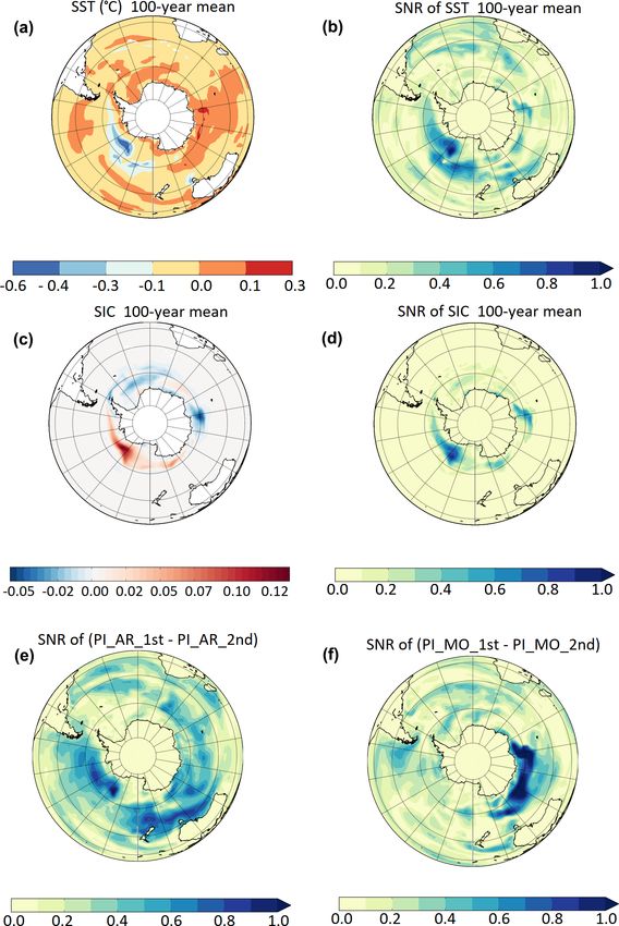
invalidate the analysis presented above. The sea ice area is In Fig. 11, (PIMO − PIAR ) differences materialize into spa-
an integral computed over a limited area, and not a mean tial patterns that are signatures of physical processes. SST
computed on a globally uniform surface (like all the other (Fig. 11a, b) and SIC (Fig. 11c, d) anomalies are the largest
in West Antarctica where ENSO teleconnection patterns are
1 Note that, for readability, the ticks of the x axes in Figs. 4d expected; they correspond to regions where SNR becomes
to 9d were equally spaced. This partially masks the power-law be- equal to or larger than 1. This suggests that (PIMO − PIAR )
haviour discussed in the paper, which can be better detected when differences are driven by two different ENSO regimes (the
the natural x axes are used. connection between SIC (and SST) anomalies in the South-
www.geosci-model-dev.net/13/139/2020/ Geosci. Model Dev., 13, 139–154, 2020150 M.-V. Guarino et al.: Machine dependence and reproducibility for coupled climate simulations
Figure 10. Log–log plots of SST (a), SAT (b), SW TOA (c), LW TOA (d), and P (e) representing maximum (PIMO − PIAR ) differences as a
function of the timescale. All the variables were averaged globally (green circles) and over the SH (red crosses) and NH (yellow diamonds).
The straight lines represent the best-fit lines for the data obtained by linear regression.
ern Hemisphere and ENSO has been widely documented in sembles the one shown by (PIMO − PIAR ) differences
the literature; e.g. Kwok and Comiso, 2002; Liu et al., 2002; in Fig. 11b. Thus, we conclude that differences between
Turner, 2004; Welhouse et al., 2016; Pope et al., 2017). ARCHER and MO are comparable to differences between
This hypothesis is confirmed by the ENSO signal in ensemble members run on a single machine.
Fig. 12. A few times, a strong El Niño (La Niña) event in As for PIMO , in Fig. 11f large differences (and SNR >
PIMO corresponds to a strong La Niña (El Niño) event in 1) between the two ensemble members are found in East
PIAR . This opposite behaviour enlarges SIC (and SST) dif- Antarctica. While this suggests that in this case a climate
ferences between the two runs and strengthens the µMO−AR process other than ENSO is in action, the large SNR con-
signal, resulting in a strong SNR. firms that 100 years is too short a length for constant-forcing
As ENSO provides a medium-frequency modulation of the HadGEM3-GC3.1 simulations even on the same machine.
climate system, it is not surprising that it takes longer than In summary, the analysis above confirms that (PIMO −
100 years for its variability to be fully represented (see e.g. PIAR ) differences, while triggered by the computing environ-
Wittenberg, 2009). ment, are largely dominated by the internal variability as they
Finally, we want to know whether the two ENSO regimes persist among ensemble members on the same machine (in
in PIMO and PIAR are a reflection of the different computing Fig. 11 SNR > 1).
environment or solely the result of natural variability (i.e. if
a similar behaviour can be detected for simulations run on
the same machine). This can be done by splitting the 200- 5 Discussion and conclusions
year simulations in two segments and assuming that each
In this paper, the effects of different computing environments
100-year period of PIMO and PIAR is a member of an ensem-
on the reproducibility of coupled climate model simulations
ble of size two. Therefore, the ARCHER ensemble is made
are discussed. Two versions of the UK CMIP6 PI control
of PIAR 1st and PIAR 2nd, and the MO ensemble comprises
simulation, one run on the UK Met Office supercomputer
PIMO 1st and PIMO 2nd.
(MO) (PIMO ) and the other run on the ARCHER (PIAR ) HPC
Figure 11e and f show the signal-to-noise ratio corre-
platform, were used to investigate the impact of machine-
sponding to SST differences between PIAR 1st and PIAR 2nd
dependent processes of the N96ORCA1 HadGEM3-GC3.1
and between PIMO 1st and PIMO 2nd. In Fig. 11e, the SNR
model.
pattern exhibited by the ARCHER ensemble members re-
Geosci. Model Dev., 13, 139–154, 2020 www.geosci-model-dev.net/13/139/2020/M.-V. Guarino et al.: Machine dependence and reproducibility for coupled climate simulations 151
Figure 11. The 100-year means and corresponding SNR of (PIMO − PIAR ) differences for SH SST (a, b) and SH SIC (c, d). Panels (e) and
(f) show SNR of (PIAR 1st − PIAR 2nd) and (PIMO 1st − PIMO 2nd) differences for SH SST, respectively.
Discrepancies between the means of key climate variables Although the two versions of the same PI control simula-
(SST, SIA / SIC, SAT, SW TOA, LW TOA, and P ) were tion do not bit-compare, we found that the long-term statis-
analysed at different timescales, from decadal to centennial tics of the two runs are similar and that, on multi-centennial
(see Sect. 3.2 for details on methodology). timescales, the considered variables show a signal-to-noise
ratio (SNR) less than 1. We conclude that in order for PIMO
www.geosci-model-dev.net/13/139/2020/ Geosci. Model Dev., 13, 139–154, 2020152 M.-V. Guarino et al.: Machine dependence and reproducibility for coupled climate simulations
Figure 12. The Niño 3.4 index for PIMO and PIAR . A 3-month running mean was applied to the ENSO signal, and values greater and smaller
than or equal to ±0.5 are shaded in orange and green.
and PIAR to be statistically indistinguishable, a 200-year av- the HadGEM3-GC3.1 model (on the same or on a different
eraging period must be used for the analysis of the results. machine). While this result is not unexpected per se, it is rele-
This indicates that simulations using the HadGEM3-GC3.1 vant to CMIP6 experiments as CMIP6 protocols recommend
model are reproducible on different HPC platforms (in their a minimum simulation length of 100 years (or less) for many
mean climate properties), provided that a sufficiently long of the MIP experiments.
simulation length is used. This result has immediate implications for members of the
Additionally, the relationship between global mean differ- UK CMIP6 community who will run individual MIP exper-
ences and timescale exhibits a ≈ 2/3 power-law behaviour, iments on the ARCHER HPC platform and will compare
regardless the physical quantity considered, that approaches results against the reference PI simulation run on the MO
a plateau near the 200-year timescale. Thus, there is a con- platform by the UK Met Office. The magnitude of (PIMO
sistent time-dependent scaling of (PIMO − PIAR ) differences − PIAR ) differences presented in this paper should be re-
across the whole climate simulation so that variables con- garded as threshold values below which differences between
verge toward their true values at the same rate, independently ARCHER and MO simulations must be interpreted with cau-
of the physical processes that they represent. tion (as they might be the consequence of a wrong sampling
Larger inconsistencies between the two runs were found of the model internal variability rather than the climate re-
for shorter timescales (at which SNR ≥ 1), the largest be- sponse to a different forcing).
ing at decadal timescales. For example, when a 10-year av- In light of our results, our recommendation to the UK
eraging period is used, discrepancies between the runs can MIPs studying the climate response to different forcings is
be up to |0.2| ◦ C global mean air temperature anomalies, or to run HadGEM3-GC3.1 for at least 200 years, even when
|1.2| million km2 Southern Hemisphere sea ice area anoma- CMIP6 minimum requirements are 100 years (see, for exam-
lies. The observed differences are a direct consequence of ple, the PMIP protocols; Otto-Bleisner et al., 2017).
the different sampling of the internal variability when the Finally, although the quantitative analysis presented in this
same climate simulation is run on different machines. They paper applies strictly to HadGEM3-GC3.1 constant-forcing
become approximately zero when a 200-year averaging pe- climate simulations only, this study has the broader purpose
riod is used, confirming that the overall physical behaviour of increasing awareness in the climate modelling community
of the model was not affected by the different computing en- of the subject of the machine dependence of climate simula-
vironments. tions.
On a 100-year timescale, large SST and SIC differences
(with SNR ≥ 1) were found where ENSO teleconnection pat-
terns are expected. Medium-frequency climate processes like Code availability. Access to the model code used in the paper has
ENSO need longer than 100 years to be fully represented. been granted to the editor. The source code of the UM is available
Thus, a 100-year constant-forcing simulation may not be under licence. To apply for a licence, go to http://www.metoffice.
long enough to correctly capture the internal variability of gov.uk/research/modelling-systems/unified-model (UK Met Office,
2020). JULES is available under licence free of charge; see
Geosci. Model Dev., 13, 139–154, 2020 www.geosci-model-dev.net/13/139/2020/M.-V. Guarino et al.: Machine dependence and reproducibility for coupled climate simulations 153
https://jules-lsm.github.io/ (Joint UK Land Environment Simula- tal design and organization, Geosci. Model Dev., 9, 1937–1958,
tor, 2020). The NEMO model code is available from http://www. https://doi.org/10.5194/gmd-9-1937-2016, 2016.
nemo-ocean.eu (NEMO Consortium, 2020). The model code for Good, P., Andrews, T., Chadwick, R., Dufresne, J.-L., Gregory,
CICE can be downloaded from https://code.metoffice.gov.uk/trac/ J. M., Lowe, J. A., Schaller, N., and Shiogama, H.: nonlin-
cice/browser (CICE Consortium, 2020). MIP contribution to CMIP6: model intercomparison project for
non-linear mechanisms: physical basis, experimental design and
analysis principles (v1.0), Geosci. Model Dev., 9, 4019–4028,
Data availability. Access to the data used in the paper has been https://doi.org/10.5194/gmd-9-4019-2016, 2016.
granted to the editor. The CMIP6 PI simulation run by the UK Gregory, J. M., Bouttes, N., Griffies, S. M., Haak, H., Hurlin, W. J.,
Met Office will be made available on the Earth System Grid Fed- Jungclaus, J., Kelley, M., Lee, W. G., Marshall, J., Romanou,
eration (ESGF) (https://cera-www.dkrz.de/WDCC/ui/cerasearch/ A., Saenko, O. A., Stammer, D., and Winton, M.: The Flux-
cmip6?input=CMIP6.CMIP.MOHC.HadGEM3-GC31-LL, Anomaly-Forced Model Intercomparison Project (FAFMIP) con-
https://doi.org/10.22033/ESGF/CMIP6.419; Ridley et al., 2018a), tribution to CMIP6: investigation of sea-level and ocean climate
the data repository for all CMIP6 output. CMIP6 outputs are change in response to CO2 forcing, Geosci. Model Dev., 9, 3993–
expected to be public by 2020. The dataset used for the analysis 4017, https://doi.org/10.5194/gmd-9-3993-2016, 2016.
of the PI simulation ported to ARCHER can be shared, under Haarsma, R. J., Roberts, M. J., Vidale, P. L., Senior, C. A., Bellucci,
request, via the CEDA platform (https://help.ceda.ac.uk, last A., Bao, Q., Chang, P., Corti, S., Fučkar, N. S., Guemas, V., von
access: 13 January 2020). Please contact the authors. Hardenberg, J., Hazeleger, W., Kodama, C., Koenigk, T., Leung,
L. R., Lu, J., Luo, J.-J., Mao, J., Mizielinski, M. S., Mizuta, R.,
Nobre, P., Satoh, M., Scoccimarro, E., Semmler, T., Small, J.,
Author contributions. MVG ran the simulation on the ARCHER and von Storch, J.-S.: High Resolution Model Intercomparison
supercomputer, designed and carried out the tests in Sect. 2, and Project (HighResMIP v1.0) for CMIP6, Geosci. Model Dev., 9,
analysed all simulation results with the contribution of LCS and DS. 4185–4208, https://doi.org/10.5194/gmd-9-4185-2016, 2016.
GL and RH ported the HadGEM3 PI simulation to the ARCHER su- Hong, S.-Y., Koo, M.-S., Jang, J., Esther Kim, J.-E., Park, H., Joh,
percomputer, provided technical support, and advised on the nature M.-S., Kang, J.-H., and Oh, T.-J.: An evaluation of the soft-
of machine-dependent processes. All authors revised the paper. ware system dependency of a global atmospheric model, Mon.
Weather Rev., 141, 4165–4172, 2013.
Joint UK Land Environment Simulator: JULES, available at: https:
//jules-lsm.github.io/, last access: 13 January 2020.
Competing interests. The authors declare that they have no conflict
Kravitz, B., Robock, A., Tilmes, S., Boucher, O., English, J. M.,
of interest.
Irvine, P. J., Jones, A., Lawrence, M. G., MacCracken, M.,
Muri, H., Moore, J. C., Niemeier, U., Phipps, S. J., Sillmann, J.,
Storelvmo, T., Wang, H., and Watanabe, S.: The Geoengineering
Acknowledgements. We would like to thank the two anonymous Model Intercomparison Project Phase 6 (GeoMIP6): simulation
referees and the topical editor, Sophie Valcke, for their time and design and preliminary results, Geosci. Model Dev., 8, 3379–
their valuable comments. 3392, https://doi.org/10.5194/gmd-8-3379-2015, 2015.
Maria-Vittoria Guarino and Louise C. Sime acknowledge the Kuhlbrodt, T., Jones, C. G., Sellar, A., Storkey, D., Blockley, E.,
financial support of NERC research grants NE/P013279/1 and Stringer, M., Hill, R., Graham, T., Ridley, J., Blaker, A., Calvert,
NE/P009271/1. This work used the ARCHER UK National Su- D., Copsey, D., Ellis, R., Hewitt, H., Hyder, P., Ineson, S., Mulc-
percomputing Service (http://www.archer.ac.uk, last access: 13 Jan- ahy, J., Siahaan, A., and Walton, J.: The Low-Resolution Version
uary 2020). The authors acknowledge the use of the UK Met Office of HadGEM3 GC3. 1: Development and Evaluation for Global
supercomputing facility in providing data for model comparisons. Climate, J. Adv. Model. Earth Sy., 10, 2865–2888, 2018.
Kwok, R. and Comiso, J. C.: Spatial patterns of variability
in Antarctic surface temperature: Connections to the South-
Financial support. This research has been supported by NERC ern Hemisphere Annular Mode and the Southern Oscillation,
(grant nos. NE/P013279/1 and NE/P009271/1). Geophys. Res. Lett., 29, https://doi.org/10.1029/2002GL015415,
2002.
Liu, J., Yuan, X., Rind, D., and Martinson, D. G.: Mechanism study
Review statement. This paper was edited by Sophie Valcke and re- of the ENSO and southern high latitude climate teleconnections,
viewed by two anonymous referees. Geophys. Res. Lett., 29, https://doi.org/10.1029/2002GL015143,
2002.
Liu, L., Li, R., Zhang, C., Yang, G., Wang, B., and Dong, L.: En-
hancement for bitwise identical reproducibility of Earth system
References modeling on the C-Coupler platform, Geosci. Model Dev. Dis-
cuss., 8, 2403–2435, https://doi.org/10.5194/gmdd-8-2403-2015,
CICE Consortium: CICE, available at: https://github.com/ 2015a.
CICE-Consortium last access: 13 January 2020. Liu, L., Peng, S., Zhang, C., Li, R., Wang, B., Sun, C., Liu, Q.,
Eyring, V., Bony, S., Meehl, G. A., Senior, C. A., Stevens, B., Dong, L., Li, L., Shi, Y., He, Y., Zhao, W., and Yang, G.: Impor-
Stouffer, R. J., and Taylor, K. E.: Overview of the Coupled tance of bitwise identical reproducibility in earth system mod-
Model Intercomparison Project Phase 6 (CMIP6) experimen-
www.geosci-model-dev.net/13/139/2020/ Geosci. Model Dev., 13, 139–154, 2020154 M.-V. Guarino et al.: Machine dependence and reproducibility for coupled climate simulations eling and status report, Geosci. Model Dev. Discuss., 8, 4375– Song, Z., Qiao, F., Lei, X., and Wang, C.: Influence of par- 4400, https://doi.org/10.5194/gmdd-8-4375-2015, 2015b. allel computational uncertainty on simulations of the Cou- Loeve, M.: Elementary probability theory, in: Probability Theory I, pled General Climate Model, Geosci. Model Dev., 5, 313–319, Springer, 1–52, 1977. https://doi.org/10.5194/gmd-5-313-2012, 2012. Lorenz, E. N.: Deterministic nonperiodic flow, J. Atmos. Sci., 20, Turner, J.: The El Niño–Southern Oscillation and Antarctica, Int. J. 130–141, 1963. Climatol., 24, 1–31, 2004. Madec, G. and the NEMO Team: NEMO ocean engine, UK Met Office: Unified Model, available at: http://www.metoffice. available at: https://epic.awi.de/id/eprint/39698/1/NEMO_book_ gov.uk/research/modelling-systems/unified-model, last access: v6039.pdf (last access: 13 January 2020), 2015. 13 January 2020. Menary, M. B., Kuhlbrodt, T., Ridley, J., Andrews, M. B., Dimdore- Walters, D., Boutle, I., Brooks, M., Melvin, T., Stratton, R., Vosper, Miles, O. B., Deshayes, J., Eade, R., Gray, L., Ineson, S., S., Wells, H., Williams, K., Wood, N., Allen, T., Bushell, A., Mignot, J., Roberts, C. and Robson, J., Wood, R., and Xavier, P.: Copsey, D., Earnshaw, P., Edwards, J., Gross, M., Hardiman, Preindustrial Control Simulations With HadGEM3-GC3. 1 for S., Harris, C., Heming, J., Klingaman, N., Levine, R., Man- CMIP6, J. Adv. Model. Earth Sy., 10, 3049–3075, 2018. ners, J., Martin, G., Milton, S., Mittermaier, M., Morcrette, C., NEMO Consortium: NEMO, available at: https://www. Riddick, T., Roberts, M., Sanchez, C., Selwood, P., Stirling, nemo-ocean.eu/, last access: 13 January 2020. A., Smith, C., Suri, D., Tennant, W., Vidale, P. L., Wilkinson, Otto-Bliesner, B. L., Braconnot, P., Harrison, S. P., Lunt, D. J., J., Willett, M., Woolnough, S., and Xavier, P.: The Met Office Abe-Ouchi, A., Albani, S., Bartlein, P. J., Capron, E., Carlson, Unified Model Global Atmosphere 6.0/6.1 and JULES Global A. E., Dutton, A., Fischer, H., Goelzer, H., Govin, A., Hay- Land 6.0/6.1 configurations, Geosci. Model Dev., 10, 1487– wood, A., Joos, F., LeGrande, A. N., Lipscomb, W. H., Lohmann, 1520, https://doi.org/10.5194/gmd-10-1487-2017, 2017. G., Mahowald, N., Nehrbass-Ahles, C., Pausata, F. S. R., Peter- Welhouse, L. J., Lazzara, M. A., Keller, L. M., Tripoli, G. J., and schmitt, J.-Y., Phipps, S. J., Renssen, H., and Zhang, Q.: The Hitchman, M. H.: Composite analysis of the effects of ENSO PMIP4 contribution to CMIP6 – Part 2: Two interglacials, scien- events on Antarctica, J. Climate, 29, 1797–1808, 2016. tific objective and experimental design for Holocene and Last Williams, K., Copsey, D., Blockley, E., Bodas-Salcedo, A., Calvert, Interglacial simulations, Geosci. Model Dev., 10, 3979–4003, D., Comer, R., Davis, P., Graham, T., Hewitt, H., Hill, R., Hyder, https://doi.org/10.5194/gmd-10-3979-2017, 2017. P., Ineson, S., Johns, T. C., Keen, A. B., Lee, R. W., Megann, Pope, J. O., Holland, P. R., Orr, A., Marshall, G. J., and Phillips, T.: A., Milton, S. F., Rae, J. G. L., Roberts, M. J., Scaife, A. A., The impacts of El Niño on the observed sea ice budget of West Schiemann, R., Storkey, D., Thorpe, L., Watterson, I. G., Walters, Antarctica, Geophys. Res. Lett., 44, 6200–6208, 2017. D. N., West, A., Wood, R. A., Woollings, T., and Xavier, P. K.: Ridley, J., Menary, M., Kuhlbrodt, T., Andrews, M., and An- The Met Office global coupled model 3.0 and 3.1 (GC3.0 and drews, T.: MOHC HadGEM3-GC31-LL model output pre- GC3.1) configurations, J. Adv. Model. Earth Sy., 10, 357–380, pared for CMIP6 CMIP, Earth System Grid Federation, 2018. https://doi.org/10.22033/ESGF/CMIP6.419, 2018a. Wittenberg, A. T.: Are historical records sufficient to con- Ridley, J. K., Blockley, E. W., Keen, A. B., Rae, J. G. L., strain ENSO simulations?, Geophys. Res Lett., 36, L12702, West, A. E., and Schroeder, D.: The sea ice model compo- https://doi.org/10.1029/2009GL038710, 2009. nent of HadGEM3-GC3.1, Geosci. Model Dev., 11, 713–723, https://doi.org/10.5194/gmd-11-713-2018, 2018b. Geosci. Model Dev., 13, 139–154, 2020 www.geosci-model-dev.net/13/139/2020/
You can also read