Ionospheric response to solar extreme ultraviolet radiation variations: comparison based on CTIPe model simulations and satellite measurements
←
→
Page content transcription
If your browser does not render page correctly, please read the page content below
Ann. Geophys., 39, 341–355, 2021
https://doi.org/10.5194/angeo-39-341-2021
© Author(s) 2021. This work is distributed under
the Creative Commons Attribution 4.0 License.

Ionospheric response to solar extreme ultraviolet radiation
variations: comparison based on CTIPe model simulations and
satellite measurements
Rajesh Vaishnav1 , Erik Schmölter2 , Christoph Jacobi1 , Jens Berdermann2 , and Mihail Codrescu3
1 LeipzigInstitute for Meteorology, Universität Leipzig, Stephanstr. 3, 04103 Leipzig, Germany
2 German Aerospace Center, Kalkhorstweg 53, 17235 Neustrelitz, Germany
3 Space Weather Prediction Centre, National Oceanic and Atmospheric Administration, Boulder, Colorado, USA

Correspondence: Rajesh Vaishnav (rajesh_ishwardas.vaishnav@uni-leipzig.de)

Received: 5 December 2020 – Discussion started: 11 December 2020
Revised: 9 February 2021 – Accepted: 24 February 2021 – Published: 6 April 2021

Abstract. The ionospheric total electron content (TEC) pro-     1   Introduction
vided by the International GNSS Service (IGS) and the TEC
simulated by the Coupled Thermosphere Ionosphere Plas-
masphere Electrodynamics (CTIPe) model have been used           The ionospheric day-to-day variations are mainly con-
to investigate the delayed ionospheric response against solar   trolled by fluctuations of solar extreme ultraviolet/ultraviolet
flux and its trend during the years 2011 to 2013. The analy-    (EUV/UV) radiation responsible for photoionization and
sis of the distinct low-latitude and midlatitude TEC response   photo-dissociation processes, lower atmospheric forcing, and
over 15◦ E shows a better correlation of observed TEC and       space weather events such as geomagnetic storms. During
the solar radio flux index F10.7 in the Southern Hemisphere     geomagnetically and meteorologically quiet conditions, the
compared to the Northern Hemisphere. Thus, a significant        electron density gradually increases after sunrise, with a
hemispheric asymmetry is observed.                              maximum around 14:00 LT due to photochemical processes,
   The ionospheric delay estimated using model-simulated        and starts decreasing thereafter due to the combined effect of
TEC is in good agreement with the delay estimated for ob-       production and strong recombination, continuing after sunset
served TEC against the flux measured by the Solar Dynam-        due to recombination processes.
ics Observatory (SDO) extreme ultraviolet (EUV) Variabil-          The solar radiation flux varies at different timescales, in-
ity Experiment (EVE). The average delay for the observed        cluding the diurnal cycle, the 27 d solar rotation period,
(modeled) TEC is 17(16) h. The average delay calculated for     and the prominent 11-year solar cycle. This results in cor-
observed and modeled TEC is 1 and 2 h longer in the South-      responding variations in composition and dynamics of the
ern Hemisphere compared to the Northern Hemisphere.             thermosphere–ionosphere (T–I) system (Hedin, 1984). The
   Furthermore, the observed TEC is compared with the           T–I system is highly variable with location and time, depend-
modeled TEC simulated using the SOLAR2000 and EUVAC             ing on the solar activity and geomagnetic disturbances.
flux models within CTIPe over northern and southern hemi-          The photoionization processes in the ionosphere cause
spheric grid points. The analysis suggests that TEC simu-       different variations, including short-term variability at the
lated using the SOLAR2000 flux model overestimates the          timescale of the 27 d solar rotation or seasonal variations.
observed TEC, which is not the case when using the EUVAC        Past studies on the effect of solar radiation variations at dif-
flux model.                                                     ferent timescales have been based on the total electron con-
                                                                tent (TEC, frequently given in TECU; 1 TECU= 1016 elec-
                                                                trons m−2 ), peak electron density (NmF2, cm−3 ), and the
                                                                corresponding height (HmF2, km) (e.g., Jakowski et al.,
                                                                1991; Afraimovich et al., 2008; Lee et al., 2012; Jacobi

Published by Copernicus Publications on behalf of the European Geosciences Union.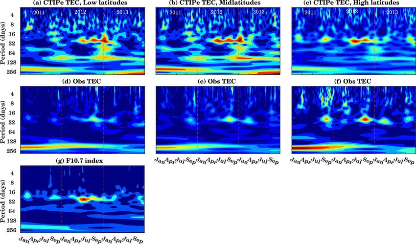
342                                              R. Vaishnav et al.: Ionospheric response to solar EUV radiation variations

et al., 2016; Schmölter et al., 2018, 2020; Vaishnav et al.,      model was represented by the F10.7 index (Ren et al., 2018;
2018, 2019; Ren et al., 2018, and references therein).            Vaishnav et al., 2018).
   The annual contributions to the mean TEC variability have         The most commonly used solar proxy for ionizing irradi-
a stronger impact on the Southern Hemisphere, whereas the         ance is the solar radio flux at 10.7 cm (F10.7 index, given in
semi-annual contributions have similar phase and amplitude        solar flux units (sfu); 1 sfu = 10−22 Wm−2 Hz−1 ) (Tapping,
at conjugate points, suggesting close coupling between the        1987). Most of the T–I models use a modified F10.7 index
ionosphere and thermosphere (Liu et al., 2009). Mendillo          (e.g., the average of daily and 41 or 81 d averages) to calcu-
et al. (2002) suggested that both annual and semi-annual vari-    late the model EUV spectra based on reference spectra. Sev-
ations of NmF2 are largely caused by changes in the neutral       eral authors have reported that a modified F10.7 index, which
composition, which are driven by the global thermospheric         includes both short-term and long-term variability, is a better
circulation.                                                      proxy for ionizing irradiance than F10.7 directly (Richards
   Solar proxies are frequently used to represent the solar ac-   et al., 1994). There are several empirical models available,
tivity. Among them are the F10.7 index, the Mg-II index, and      such as the SOLAR2000 (Tobiska et al., 2000) and EUVAC
the He-II index. Furthermore, attempts have been made to          flux model (Richards et al., 1994), to calculate the irradiance.
determine simple proxies for global TEC variability based            Profiles of the delayed ionospheric response dependent on
on these indices (e.g., Unglaub et al., 2011). These prox-        latitude have been calculated in previous studies (Lee et al.,
ies have been compared to the ionospheric parameters at the       2012; Ren et al., 2018), and the influence of seasonal varia-
timescale of the 27 d solar rotation. An ionospheric delay of     tions and geomagnetic activity on both hemispheres has also
about 1–2 d has been reported (e.g., Jakowski et al., 1991; Ja-   been characterized (Schmölter et al., 2020). The complex-
cobi et al., 2016). Using a more precise and higher temporal      ity of the seasonal variations and associated anomalies has
resolution solar flux, an ionospheric delay of about 17–19 h      been investigated in other studies for ionospheric parame-
has been reported by Schmölter et al. (2018). The spatial and     ters like TEC (Romero-Hernandez et al., 2018). Such sea-
seasonal effects on the ionospheric delay have been further       sonal anomalies were observed in the F2 region associated
investigated in detail by Schmölter et al. (2020) using Eu-       with higher electron density in winter than in summer during
ropean and Australian locations. Their study highlighted the      daytime (the so-called winter or seasonal anomaly), during
role of geomagnetic activity in the ionospheric delay.            equinoxes than during solstices (semi-annual anomaly), and
   To investigate the process associated with the ionospheric     in December than in June (annual or non seasonal anomaly)
delay, Jakowski et al. (1991) used a one-dimensional numer-       (Balan et al., 1998; Zou et al., 2000; Romero-Hernandez
ical model between 100 and 250 km altitude with simpli-           et al., 2018). However, seasonal variations have not yet been
fying assumptions. They suggested that a delay of approx-         analyzed for the ionospheric delay.
imately 2 d arises in atomic oxygen at 180 km due to photo-          The ionospheric electron density (or ion density) is mainly
dissociation and transport processes. This hypothesis has         controlled by the photoionization, the loss through recom-
yet to be confirmed with comprehensive ionospheric mod-           bination, and transport processes. Transport processes play
els such as CTIPe (Coupled Thermosphere Ionosphere Plas-          a significant role in the T–I composition and are responsi-
masphere Electrodynamics). Ren et al. (2018) investigated         ble for the plasma distribution, possibly leading to the ob-
the ionospheric delay using observations and modeling. They       served ionospheric anomalies. Fuller-Rowell (1998) suggests
emphasized the role of the [O]/[N2 ] ratio in the ionospheric     a possible mechanism associated with the seasonal anomaly
delay. Vaishnav et al. (2018) suggested the possible role of      through the neutral wind.
transport processes in the ionospheric delay.                        This study aims to analyze the ionospheric TEC varia-
   During the past decades, more improved physics-based           tions in both the Northern and Southern Hemisphere during
T–I models have been developed which are able to char-            a moderate solar activity during the inclining phase of so-
acterize ionospheric dynamics. Among them are the Cou-            lar cycle 24 (2011–2013). We use GNSS data from 70◦ S
pled Thermosphere Ionosphere Plasmasphere Electrody-              to 70◦ N latitude at 15◦ E longitude due to better coverage
namics model (CTIPe; Fuller-Rowell and Rees, 1983;                with ground measurements in TEC maps. The observed TEC
Codrescu et al., 2012), the Thermosphere–Ionosphere–              is compared with the model-simulated TEC using different
Electrodynamics General Circulation Model (TIE-GCM;               solar EUV flux models. The ionospheric delay against solar
Richmond et al., 1992), and the Global Ionosphere Ther-           EUV flux has been investigated by Schmölter et al. (2020)
mosphere Model (GITM; Ridley et al., 2006). Furthermore,          using TEC observations. Therefore, the focus of the present
some extended Earth system models like WACCM-X (Liu               study is laid on the ability to reproduce the ionospheric delay
et al., 2018) and the Ground-to-topside model of Atmosphere       using the CTIPe model at 15◦ E.
and Ionosphere for Aeronomy (GAIA; Jin et al., 2012; Liu             In Sect. 2, we introduce the data sources and the CTIPe
et al., 2020) include T–I dynamics. Based on the results of       model. In Sect. 3, we investigate the TEC variability and a
the T–I model, an ionospheric lag against variations of the       possible relationship with F10.7 index variations and com-
solar EUV could be identified, whereby the EUV entry in the       pare TEC simulated with the different solar EUV flux mod-
                                                                  els. In Sect. 4, we summarize our conclusions.

Ann. Geophys., 39, 341–355, 2021                                                  https://doi.org/10.5194/angeo-39-341-2021
R. Vaishnav et al.: Ionospheric response to solar EUV radiation variations                                                     343

                                                                    radiance measurements from the TIMED Solar Extreme Ul-
                                                                    traviolet Experiment (SEE) instrument have been available
                                                                    since 22 January 2002 (Woods et al., 2005). The SEE instru-
                                                                    ment is designed to measure the soft X-rays and EUV ra-
                                                                    diation from 0.1 to 194 nm, with resolution and accuracy of
                                                                    0.1 nm and approximately 10 %–20 %. SEE includes two in-
                                                                    struments, the EUV grating spectrograph and the soft X-ray
                                                                    (XUV) photometer system (Woods et al., 2000). Here we use
                                                                    daily values of solar irradiance integrated from 1 to 105 nm
                                                                    wavelength. The TIMED SEE observations are used for com-
                                                                    parison with the empirical solar flux models, SOLAR2000
                                                                    and EUVAC.
                                                                       Furthermore, the Solar Dynamics Observatory (SDO)
                                                                    EUV Variability Experiment (EVE) provides a continuous
                                                                    high-resolution spectrum with a wavelength range from 0.1
                                                                    to 120 nm, a spectral resolution of 0.1 nm, and a temporal
                                                                    resolution of 20 s. (Woods et al., 2010; Pesnell et al., 2011).
                                                                    The high-resolution EUV observations provided by the SDO
                                                                    EVE satellite have been used to calculate an ionosphere de-
                                                                    lay in TEC.
                                                                       Solar proxies are mostly used as a solar activity represen-
                                                                    tation in thermosphere–ionosphere models. Hence, we also
                                                                    use the daily F10.7 index for our analysis.

                                                                    2.3   CTIPe model

                                                                    The CTIPe model is a global, first-principle, three-
Figure 1. IGS stations around 15◦ E. The dashed black line repre-
                                                                    dimensional        numerical,      physics-based      coupled
sents the geomagnetic equator.
                                                                    thermosphere–ionosphere–plasmasphere model, which
                                                                    self-consistently solves the primitive equations of continuity,
                                                                    momentum, and energy to calculate wind components,
2     Observations and model
                                                                    global temperature, and the composition of neutrals, which
2.1    TEC observations                                             is further used to calculate plasma production, loss, and
                                                                    transport. The model consist of four components, namely
In this paper, we use TEC data from 70◦ S to 70◦ N latitude         a neutral thermosphere model (Fuller-Rowell and Rees,
at 15◦ E from the International GNSS Service (IGS) provided         1980), a midlatitude and high-latitude ionosphere con-
by NASA’s CDDIS (Noll, 2010), which are available at 1 h            vection model (Quegan et al., 1982), a plasmasphere and
time resolution and with a latitude–longitude resolution of         low-latitude ionosphere model (Millward et al., 1996), and
2.5◦ × 5◦ (Hernández-Pajares et al., 2009). The accuracy of         an electrodynamics model (Richmond et al., 1992). The
IGS TEC maps is given with 2–8 TECU (Chen et al., 2020).            calculations are performed with 2◦ /18◦ latitude/longitude
There are only few IGS stations in the Southern Hemisphere,         resolution. In the vertical direction, the atmosphere is
but in the Northern Hemisphere (European region), there are         divided into 15 levels in logarithmic pressure at an interval
several ground stations located around 15◦ E, as shown in           of one scale height, starting from a lower boundary at 1 Pa
Fig. 1.                                                             (about 80 km altitude) to above 500 km altitude at pressure
                                                                    level 15. The high-latitude ionosphere (above 55◦ N or S)
2.2    Solar EUV radiation                                          and the midlatitude–low-latitude ionosphere–plasmasphere
                                                                    components have been implemented as separate modules.
Several solar proxies are available that have frequently been          The numerical solution of the composition equation and
used in previous studies to represent the solar activity level      the energy and momentum equations describe transport, tur-
compared to the ionospheric parameters before the space             bulence, and diffusion of atomic oxygen, molecular oxy-
age and due to the unavailability of direct solar EUV mea-          gen, and nitrogen (Fuller-Rowell and Rees, 1983). To run
surements. Continuous time series of the solar EUV spec-            the model, external inputs are required like solar UV and
trum itself, however, have been available since the launch of       EUV, Weimer electric field, TIROS/NOAA auroral precipi-
the NASA Thermosphere Ionosphere Mesosphere Energetics              tation, and tidal forcing from the Whole Atmosphere Model
and Dynamics (TIMED) satellite mission in 2001. Solar ir-           (WAM). The F10.7 index is used as an input solar proxy to

https://doi.org/10.5194/angeo-39-341-2021                                                    Ann. Geophys., 39, 341–355, 2021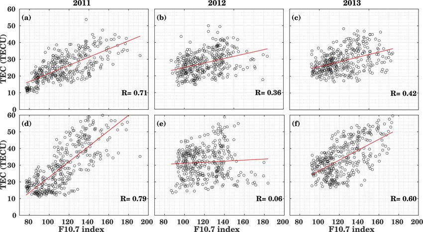
344                                             R. Vaishnav et al.: Ionospheric response to solar EUV radiation variations

calculate ionization, heating, and oxygen dissociation pro-      the flux models and the observed irradiance. The flux calcu-
cesses in the ionosphere. The CTIPe ionosphere results in-       lated by the SOLAR2000 model overestimates the observed
clude the major ion species H+ and O+ for all altitudes and      flux mostly during the Northern Hemisphere winter months,
other molecular and atomic ions, N2 , O2 , NO+ , and N+ , be-    whereas it is in good agreement during Northern Hemisphere
low 400 km. Detailed information on the CTIPe model is           summer months. The observed EUV irradiance during mod-
available in Codrescu et al. (2008, 2012) and Fernandez-         erate solar activity is comparable to the SOLAR2000 flux,
Gomez et al. (2019).                                             with a difference of about 10 % and 23 % higher than the
                                                                 EUVAC model. The EUVAC flux is about 30 % lower than
2.4     EUV representation in the CTIPe model                    the SOLAR2000 model. The correlation coefficient of EUV
                                                                 from both the EUV flux models with the observed EUV flux
2.4.1    SOLAR2000 model                                         is approximately 0.90 during the study period. In summary,
                                                                 the SOLAR2000 model is in relatively good agreement with
The SOLAR2000 model is the most recent EUV model ver-            the observed flux, while the EUVAC model underestimates
sion in a series of iterations by Tobiska et al. (2000). SO-     SOLAR2000 and the TIMED SEE flux. These results agree
LAR2000 incorporates multiple satellite and rocket measure-      with earlier comparisons (Lean et al., 2003; Woods et al.,
ments, including the AE-E satellite observations, to specify     2005; Lean et al., 2011, and references therein).
both a reference spectrum and solar variability. The EUV is         Woods et al. (2005) compared the TIMED SEE observa-
calculated using the Lyman-α flux and the F10.7 index with       tions with the flux calculated from different empirical models
the set of modeling equations. SOLAR2000 determines the          for 8 February 2002. They reported that the empirical mod-
EUV irradiance for 809 emission lines and also for 39 wave-      els are within 40 % of the SEE measurement at wavelengths
length bands.                                                    above 30 nm. The EUVAC and SOLAR2000 models agreed
                                                                 best with TIMED SEE, compared to the other models.
2.4.2    EUVAC solar flux model
                                                                    Lean et al. (2003) validated the NRLEUV model with dif-
Within CTIPe, a reference solar spectrum based on the EU-        ferent empirical models such as SOLAR2000, HFG (Hin-
VAC model (Richards et al., 1994) and the Woods and              teregger et al., 1981), and EUVAC. In absolute scales, NR-
Rottman (2002) model, driven by variations of input F10.7, is    LEUV, HFG, and EUVAC have total energies that agree
used. The EUVAC model is used between 5 and 105 nm and           within 15 %, but the SOLAR2000 absolute scale is more than
the Woods and Rottman (2002) model for 105 to 175 nm.            50 % higher. Their study reveals that long EUV wavelength
Solar flux is obtained from the reference spectra using the      (70 to 105 nm) energy contributions (about 46 % of the whole
following equation:                                              flux from 5 to 105 nm) are the main reason for the higher
                                                                 EUV flux in the SOLAR2000 model compared to other em-
f (λ) = fref (λ) [1 + A(λ)(P − 80)] ,                      (1)   pirical models.

where fref and A are the reference spectrum and solar vari-
ability factor, respectively, and P = 0.5× (F10.7 + F10.7A),
where F10.7A is the average of F10.7 over 81 d.                  3    Results and discussion
   The EUVAC model includes solar flux in 37 wavelength
bins based on the measured F74113 solar EUV reference            In the following sections, we show the results and discuss
spectrum (Hinteregger et al., 1981) and the solar cycle varia-   the TEC observations and their comparison with the modeled
tion of the flux.                                                TEC at 15◦ E. Furthermore, relations with solar radiation and
                                                                 the delayed response over both the Northern and Southern
2.4.3    Comparisons between empirical EUV irradiance
                                                                 Hemispheres are presented. Schmölter et al. (2020) have re-
         variability models and observations
                                                                 ported on a detailed investigation of the delayed ionospheric
                                                                 response over European and Australian regions. Here, we an-
We compare TIMED SEE observations with the two empir-
                                                                 alyze the delayed response at 15◦ E covering the latitudes
ical models constructed from direct proxy parameterizations
                                                                 from 70◦ S to 70◦ N and compare the response over the south-
of the EUV irradiance database, which are used to represent
                                                                 ern African region with the European region.
EUV in the CTIPe model.
                                                                    In this study we have addressed the following points:
   Figure 2 shows the modeled integrated irradiance spectra
from 5 to 105 nm calculated by both models, together with
the TIMED SEE irradiance from 2011 to 2013. The second               1. The TEC variations at moderate solar activity of solar
y axis shows the F10.7 index used to calculate the spectra in           cycle 24 are analyzed to compare the input for the de-
empirical models. In comparison to the SOLAR2000 model                  lay analysis. A characterization of these differences be-
flux and TIMED SEE, flux values calculated by the EUVAC                 tween observed and modeled TEC is important to derive
model are smaller. There is a significant difference between            further relations.

Ann. Geophys., 39, 341–355, 2021                                                   https://doi.org/10.5194/angeo-39-341-2021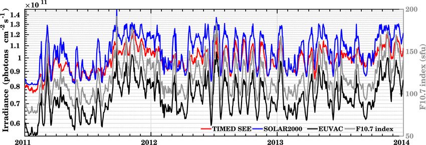
R. Vaishnav et al.: Ionospheric response to solar EUV radiation variations 345
Figure 2. Time series of 0.5 to 105 nm integrated daily irradiance from 2011 to 2013 estimated from TIMED SEE observations, SOLAR2000,
and EUVAC. The right y axis represents the F10.7 index.
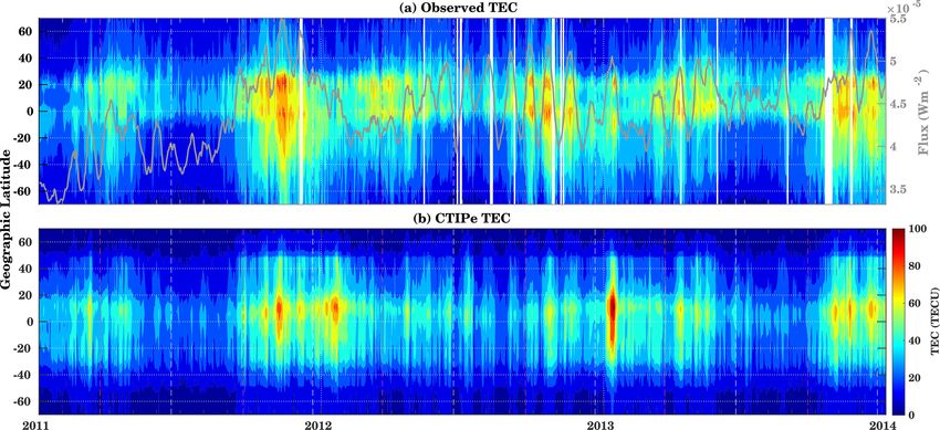
2. We used the periodicity estimation (frequency analysis) The maximum TEC is observed at the Equator and in low-
to study observed and modeled TEC characteristics in latitude regions. The TEC level reduces towards the high-
detail. latitude regions. In general, the TEC values vary latitudi-
nally depending on the northern and southern hemispheric
3. The relation between the F10.7 index and hemispheric
season. At the Equator, the plasma moves upward and redis-
TEC has been used to analyze the solar and ionospheric
tributes along the Equator, causing the fountain effect (Ap-
inputs of delay estimation.
pleton, 1946). The thermospheric wind circulations firmly
4. In our study we focus on the ionospheric delay estima- control the plasma movement. The plasma moves from the
tion as a main point of our analysis. summer hemisphere to the winter one, causing a decrease in
the F peak height, further decreasing the O/N2 ratio. The
5. The comparison of observed TEC variations with sim- TEC values in the Southern Hemisphere are higher than in
ulated TEC is done by using different flux models. In the Northern Hemisphere.
previous work it has already be shown that the solar ac- Figure 3a shows maximum TEC around the Equator dur-
tivity has the strongest impact on TEC under nominal ing the December solstice, and a minimum of TEC is ob-
conditions and is therefore significant for the derived served during the June solstice of 2011, which coincides with
delay. the minimum solar EUV flux. There are local minima during
3.1 TEC variation at moderate solar activity of solar equinoxes in 2013.
cycle 24 In comparison to observed TEC, the modeled TEC
(Fig. 3b) is lower during the spring and summer period in the
The ionospheric electron density strongly varies from day to Southern Hemisphere, while it is in better agreement during
night depending on the daily variations of solar radiation. the winter season. The bias between the modeled and ob-
Figure 3 depicts the 11:00–13:00 LT averaged midday served TEC is higher during the spring and summer season
variations in TEC for the moderate solar activity conditions in the Southern Hemisphere. In general, the modeled TEC is
from 2011 to 2013. The figure shows the comparison be- lower than the observed TEC.
tween the observed TEC and modeled TEC simulated using The variations in TEC are not only controlled by the so-
the EUVAC flux model at 15◦ E longitude. Note that at this lar radiation, but there are also other factors such as local
longitude, climatological hemispheric differences in TEC are dynamics or geomagnetic activities due to solar wind vari-
expected due to peculiarities of the magnetic field, in particu- ations, which also influence the ionospheric state (Abdu,
lar the South Atlantic Anomaly, which causes low ionization 2016). Fang et al. (2018) studied day-to-day ionospheric
in the Southern Hemisphere. variability and suggested that absolute values in TEC vari-
The TEC variations highly depend on the level of ioniza- ability at low latitudes are largely controlled by solar activ-
tion due to the solar radiation flux. The observed TEC shows ity, while for midlatitudes and high latitudes, however, solar
such variations compared to the SDO EVE-integrated flux and geomagnetic activities contribute roughly equally to the
(1–120 nm), as shown on the second y axis of Fig. 3. During absolute TEC variability.
2012, there are continuous 27 d cycles. This kind of regular A detailed comparison between the observed TEC and
variation in solar observations enables us to explore the re- modeled TEC simulated using the different solar flux models
spective ionospheric variations, which are clearly driven by (SOLAR2000 and EUVAC) during January, June, and De-
the ionization and recombination processes. cember is presented and discussed in Sect. 3.6.
https://doi.org/10.5194/angeo-39-341-2021 Ann. Geophys., 39, 341–355, 2021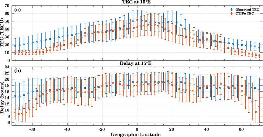
346                                              R. Vaishnav et al.: Ionospheric response to solar EUV radiation variations

Figure 3. Latitudinal variation of (a) observed TEC and (b) model-simulated TEC around noon (11:00–13:00 LT) at 15◦ E longitude. The
gray curve in panel (a) represents the SDO EVE-integrated flux (1–120 nm).

3.2   Periodicity estimation                                        mospheric forcing) is stronger. During these years, very weak
                                                                    27 d periodicity is observed. The 27 d period is stronger dur-
Solar activity varies at different timescales from minutes to       ing December and January. Pancheva et al. (1991) showed
years or even centuries. The periodic behavior in the solar         that the 27 d variation in the lower ionosphere (D region) is
proxies has been studied by various authors to explore the re-      often caused by dynamical forcing (planetary waves), partic-
sponse of the terrestrial atmosphere and especially the T–I re-     ularly in the winter season under low solar activity. A similar
gion and to investigate the connection between solar variabil-      16–32 d periodicity is observed in the F10.7 index. It is well
ity and ionospheric parameters (Jacobi et al., 2016; Vaishnav       known that the 27 d periodicity is one of the major and dom-
et al., 2019). A widely used method to analyze periodicities        inant modes of variations in the solar proxies.
in time series is the continuous wavelet transform (CWT).              As an advantage, the CWT also shows small-scale fea-
The CWT captures the impulsive events when they occur in            tures. Over low latitudes and midlatitudes, 8–16 d oscilla-
the time series (Percival and Walden, 2000; Mallat, 2009).          tions are observed to be dominant. Furthermore, another
However, the CWT also reveals lower frequency features of           high-power region is visible in the 128–256 d period, rep-
the data hidden in the time series.                                 resenting the semi-annual oscillations in both modeled and
   Here, we will investigate and compare the different tem-         observed TEC and in the F10.7 index. The semi-annual oscil-
poral patterns of observed and modeled TEC. The daily TEC           lation is mostly dominant during the period of investigation.
and F10.7 index from 2011 to 2013 are used to analyze the           Apart from it, in model-simulated TEC, a 64–128 d period is
periodic behavior of the T–I system. Figure 4 shows the con-        observed during 2012 and 2013. The oscillations are stronger
tinuous wavelet spectra of the model-simulated TEC, ob-             at low-latitude and midlatitude stations compared to high lat-
served TEC, and F10.7 for low latitudes [±30◦ ], midlatitudes       itudes.
[± (30–60◦ )], and high latitudes [± (60–70◦ )] from 2011 to           The second row of Fig. 4 shows the oscillations in the ob-
2013. Here averaged TEC is used for the low latitudes, mid-         served TEC. Here, a weak 27 d cycle is observed during De-
latitudes, and high latitudes.                                      cember, and the 128–256 d period is mostly dominant during
   The upper panels (a)–(c) of Fig. 4 show the CWT of mod-          2011 and 2012. There is a weak signature of semi-annual
eled TEC, while the middle panels (d)–(f) show the observed         oscillations during 2013. As compared to the periodicity ob-
TEC, respectively, over the different latitude bands men-           served in model-simulated TEC, the 64–128 d periodicity is
tioned in the figure title. The lower panel (g) shows the CWT       missing in the observations over all the latitudes. Further-
of F10.7.                                                           more, shorter period fluctuations can be seen, especially at
   The CWT of modeled TEC shows the dominant 16–32 d                high latitudes (Fig. 4f), with a preference for the winter sea-
oscillations during 2012. This is, however, not the case dur-       son. These may be connected with planetary wave effects
ing 2011 and 2013. During these periods, the influence of           from below (e.g. Altadill et al., 2001, 2003).
other dynamical processes in the ionosphere (e.g., lower at-

Ann. Geophys., 39, 341–355, 2021                                                     https://doi.org/10.5194/angeo-39-341-2021
R. Vaishnav et al.: Ionospheric response to solar EUV radiation variations                                                     347

   Figure 4g shows the CWT spectra of the F10.7 index. Here        3.4   Cross-correlation and delay estimation
the dominant period is 16–32 d during 2012, and a weak 16–
32 d period oscillation is observed during 2011 and 2013.          The possible relations between solar activity, geomagnetic
   In general, from the above investigation, it can be seen        activity, and ionospheric parameters have been studied by
that 16–32 d periodicity was dominant during 2012. Vaish-          several authors (e.g., Abdu, 2016; Fang et al., 2018; Vaishnav
nav et al. (2019) used cross-wavelet and Lomb–Scargle pe-          et al., 2019). However, several past studies, due to the un-
riodogram techniques to estimate the periodicity of various        availability of high-resolution datasets, used only daily res-
solar proxies and global TEC during long time series from          olution. To estimate the ionospheric delay, different iono-
2000–2016. They found that the semi-annual oscillation is          spheric parameters have been considered using daily reso-
mostly dominant during the solar maximum years 2001–               lution data; an ionospheric delay of about 1–2 d against solar
2002 and 2011–2012.                                                proxies has been reported (Jakowski et al., 1991; Jacobi et al.,
                                                                   2016; Vaishnav et al., 2019). Only recently, Schmölter et al.
3.3   Relation between F10.7 index and hemispheric                 (2020) used SDO EVE and GOES EUV fluxes to calculate
      TEC                                                          the ionospheric delay of about 17 h as a mean value based
                                                                   on hourly time resolution data. This observed delay was also
Solar activity has the strongest effect on ionospheric varia-      confirmed by numerical physics-based models (Ren et al.,
tions, especially during enhanced solar activity. The last solar   2018; Vaishnav et al., 2018).
minimum was extremely extended, and the following solar               Here, we investigate the ionospheric delay using hourly
cycle was quite weak (e.g., Huang et al., 2016), so that mete-     resolution observations and compare it with the model-
orological influences become more relevant. To examine the         simulated TEC. Figure 6 shows the cross-correlation and
effect of solar activity on TEC variations during a weak solar     a corresponding ionospheric delay calculated using SDO
cycle, we analyzed the relationship between F10.7 and mid-         EVE-observed integrated flux from the 1 to 120 nm wave-
day TEC (11:00–13:00 LT). Figure 5 shows the correlation           length region in comparison with modeled TEC at 15◦ E lon-
between TEC and F10.7 during 2011–2013 for the Northern            gitude. The modeled TEC used for these analyses has been
Hemisphere (NH; upper panels) and Southern Hemisphere              simulated using the EUVAC solar flux model and the F10.7
(SH; lower panels), indicating the correlation coefficient (R).    index as a solar input proxy to calculate the input spectra.
In order to represent the NH and SH, daily data of 40◦ N           The cross-correlation was applied on independent monthly
and 40◦ S latitudes at 15◦ E longitude have been used re-          datasets from 2011–2013, as the maximum correlation is ex-
spectively. The mean root mean square (rms) at 40◦ N is            pected during the solar rotation period. If longer periods are
6.92 TECU, and the mean rms at 40◦ S is 7.54 TECU for the          selected, the periodicity is a mixture of lower and higher so-
whole period.                                                      lar activity. Then the appearance of sunspots at different loca-
   We have calculated correlations using the observed TEC          tions on the solar disk shifts the maximum EUV emissions in
over the NH and SH. During 2011, the maximum correlation           relation to coherence with one another, for which the correla-
for all the years is observed, which amounts to R = 0.71/0.79      tion is expected to decrease. Even shorter periods can result
for the NH/SH. This suggests that midday TEC values are            in lower correlations due to the reduced sampling size, i.e., a
mainly controlled by solar EUV radiation.                          stronger impact of smaller deviations as well. Similar results
   From the current study and past publications (Romero-           have been shown by Vaishnav et al. (2019). They studied cor-
Hernandez et al., 2018), it is well known that during high         relation analysis between TEC and multiple solar proxies for
solar activity, weak correlations are observed compared to         different time periods. Their study revealed that the correla-
the moderate solar activity conditions. But during the year        tion is lower during shorter and longer periods. Better corre-
2012, the lowest correlation of about 0.06 was observed in         lations are only expected during the solar rotation period.
the SH, while the correlation was about 0.36 in the NH re-            The upper panels of Fig. 6 show the (a) cross-correlation
gion. During the year 2013, the correlation is weaker than         and (c) the ionospheric delay using the observed TEC. The
during 2011, namely about 0.42 for the NH and 0.60 for the         maximum correlation is observed during the year 2012 with
SH.                                                                about 0.5, while in 2011 and 2013 the correlation is weaker.
   In general, the correlation coefficient is higher in the        The lowest correlation is observed during the winter months
southern hemispheric region as compared to the Northern            of 2011–2012. Further, latitudinal variations are also seen in
Hemisphere during 2011 and 2013, whereas lower correla-            the correlation coefficient.
tions are observed during the year 2012. The analysis for             Figure 6c shows the cross-correlation coefficient calcu-
2012 shows some unexpected behavior over these study re-           lated using the modeled TEC and SDO-EVE flux. The corre-
gions. This unusual behavior could be due to physical and          lation coefficient is higher than the one seen in the observed
chemical processes that have an impact on the ionospheric          TEC. There are several processes that can influence the be-
state.                                                             havior of the ionosphere and the real observations such as
                                                                   lower atmospheric forcing or geomagnetic activity. But in the
                                                                   model, lower atmospheric variability is not included, except

https://doi.org/10.5194/angeo-39-341-2021                                                    Ann. Geophys., 39, 341–355, 2021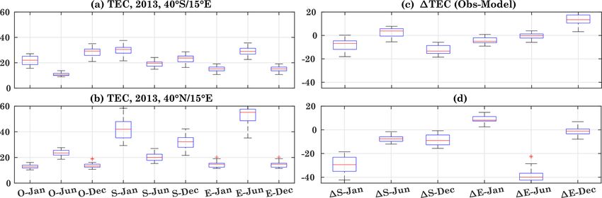
348                                                R. Vaishnav et al.: Ionospheric response to solar EUV radiation variations

Figure 4. Wavelet continuous spectra of daily modeled TEC (a–c), observed TEC (d–f) for different low latitudes [±30◦ ], midlatitudes
[±(30◦ − 60◦ )], and high latitudes [±(60◦ − 70◦ )], and (g) F10.7 index.

in a statistical sense, which affects the total variability; hence   delay is higher during December and follows the solar activ-
higher correlation is observed in modeled TEC compared to            ity.
observed TEC.                                                           In the higher latitude region (above 60◦ latitude in both
   The analysis suggests that the model can reproduce similar        hemispheres), the ionospheric delay in the model is smaller
trends and features to those shown in the observations. The          than in the observations and amounts to about 5–10 h. Si-
overall correlation coefficient in the Southern Hemisphere is        multaneously, the correlation coefficient is high at the high-
higher than in the Northern Hemisphere.                              latitude regions in the Southern Hemisphere and is about 0.4,
   Figure 6b shows the ionospheric delay calculated from the         as shown in Fig. 6c. This bias is due to the model limitations
observed TEC against the SDO flux. The ionospheric de-               such as model input, grid resolution, and insufficient physical
lay varies strongly with latitude and time. A shorter iono-          descriptions (Negrea et al., 2012).
spheric delay is observed during January as compared to                 Generally, the ionospheric delay calculated from the mod-
other months. For January, the ionospheric delay is about 13–        eled TEC is in good agreement with the observed one, and
16 h. The maximum delay is about 22 h in the low-latitude re-        it is about 17 h. Furthermore, the ionospheric delay is al-
gion during 2011 and 2012 but about 22–23 h during 2013 in           ways higher in the Northern Hemisphere as compared to the
low latitudes and midlatitudes. During 2011 the ionospheric          Southern Hemisphere. Partly negative correlation has been
delay is maximum for the winter period at the Equator with           observed in both the model and the observations. This nega-
about 22 h, while it decreases towards high latitudes. A very        tive correlation might be possible due to additional heating
low ionospheric delay of about 5–10 h is observed during Au-         sources or unknown factors such as the state of the iono-
gust 2012 for midlatitudes. An interesting feature that can be       sphere and its dominant physical processes. Another more
noted here is that the ionospheric delay increases with in-          important factor is lower atmospheric forcing, such as grav-
creasing solar activity from 2011 to 2013.                           ity or planetary wave. Gravity waves can influence the upper
   A similar analysis for the estimation of the ionospheric          atmosphere’s thermal and compositional structures. These
delay has been performed for the model-simulated TEC, as             sources might lead to changes in the ionosphere’s local dy-
shown in Fig. 6d. The CTIPe model is able to reproduce fea-          namics and contribute to additional increase and decrease in
tures seen in the observed TEC (Fig. 6b). The ionospheric            the electron density, irrespective of actual solar activity con-
                                                                     ditions.

Ann. Geophys., 39, 341–355, 2021                                                     https://doi.org/10.5194/angeo-39-341-2021
R. Vaishnav et al.: Ionospheric response to solar EUV radiation variations 349
Figure 5. Relation between F10.7 index and midday-observed TEC (11:00–13:00 LT) at 40◦ N, 15◦ E (a, b, c) and 40◦ S, 15◦ E (d, e, f) for
2011, 2012, and 2013. The red line is the linear fit.
The correlation coefficients in the Southern Hemisphere 3.5 Observed TEC variations and its comparison to
are generally higher than in the Northern Hemisphere. TEC simulated using different EUV flux models
Furthermore, to understand the mean variations of TEC
and its connection with the ionospheric delay, we calculated
the latitudinal mean observed TEC with the standard devi- To further visualize the observed daily TEC and its com-
ations and compare it with the model-simulated TEC from parison with the modeled TEC at different latitudes, the re-
2011 to 2013 as shown in Fig. 7a. The model-simulated sults are presented in the box-and-whisker plot in Fig. 8 for
TEC underestimates the observed TEC at all latitudes. As June and December 2011 to 2013. The box has lines at the
expected, the maximum TEC of about 50 TECU is ob- lower quartile, median (red line), and upper quartile values.
served at low latitudes, while model-simulated TEC is about Whiskers extend from each end of the box to the adjacent
45 TECU. The maximum bias is observed poleward of 35◦ S values in the data. Outliers beyond the whiskers are displayed
and 45◦ N, and this bias increases towards high latitudes. As using the “+” sign.
discussed in the previous sections, there are several problems To analyze the TEC variations at the grid point 40◦ S and
such as providing inputs for the model, grid resolution ef- 40◦ N, for 15◦ E each in both hemispheres during June and
fects, and insufficient physical descriptions that need to be December (left panels, a–d), we compare the observed TEC
addressed in the future to reduce the bias in the model. (O) with the modeled TEC simulated using the SOLAR2000
To see the mean latitudinal variations of ionospheric delay, (S) and the EUVAC (E) flux model for different years. The
we used the monthly delay calculated from 2011 to 2013. F10.7 index is used as the primary solar input to calculate the
The mean ionospheric delay is about 17–18 h in the obser- spectra in the model. The box plots have been generated us-
vations at low latitudes and midlatitudes, while it is about ing the daily data of June and December, respectively. The
15 h in the high-latitude regions. As compared to the delay right panels (e–h) show the differences between observed
in observations, the model-simulated delay is 1–2 h less in and modeled TEC at different corresponding locations and
the low latitudes and midlatitudes, but the difference strongly months (e–h).
increases in the high-latitude regions. Poleward of 55◦ , the The median of modeled TEC using the SOLAR2000 flux
ionospheric delay reduces to less than 10 h. model overestimates the observed TEC by about 10, 11, and
This analysis shows that the model can reproduce the iono- 7 TECU during June 2011, 2012, and 2013, respectively, at
spheric delay as seen in the observations and generally pro- 40◦ S as shown in Fig. 8a, e. A slightly smaller overestima-
duces a delay of about 18 h at middle latitudes. tion can be seen using the EUVAC flux model, with a differ-
ence of less than about 5 TECU during 2011 and 2013 and
6 TECU during 2012. Hence, both models generally show
overestimation of TEC at this latitude and month.
https://doi.org/10.5194/angeo-39-341-2021 Ann. Geophys., 39, 341–355, 2021350 R. Vaishnav et al.: Ionospheric response to solar EUV radiation variations Figure 6. Correlation coefficient (a, c) and delay estimation (b, d) using observed (a, b) and model-simulated (c, d) hourly TEC and SDO EVE-integrated flux (1–120 nm). Figure 7. (a) Daily mean TEC variations and (b) delay estimation using observed (blue) and model-simulated (red) hourly TEC and SDO EVE-integrated flux. The error bars show standard deviations of mean values. Figure 8b and f show the TEC plot and difference box plot EUVAC-model-based TEC simulation shows an underesti- at 40◦ N, 15◦ E during June. At this grid point, the observed mation of about 5–10 TECU. The modeled TEC using the TEC values are high compared to the southern hemispheric SOLAR2000 flux model is higher than the one simulated grid point. The observed TEC is quite comparable with the using the EUVAC model. A good agreement between the modeled TEC simulated using SOLAR2000 during 2011 and modeled and observed TEC can be seen at the southern and 2013. However, it shows an overestimation by 2 TECU dur- northern hemispheric grid points (Fig. 8e–f), where the bias ing 2012. In comparison to SOLAR2000-simulated TEC, the is less than 10 TECU. The analysis for December is shown in Ann. Geophys., 39, 341–355, 2021 https://doi.org/10.5194/angeo-39-341-2021
R. Vaishnav et al.: Ionospheric response to solar EUV radiation variations                                                          351

Figure 8. Box plots based on daily TEC during June and December 2011–2013 for 40◦ S and 40◦ N. The months and location are mentioned
in the figure titles. Here O, S, and E represent observed, CTIPe-SOLAR2000 flux model, and CTIPe-EUVAC flux model TEC, respectively.
The left panels show the box plots for the difference between observed TEC with the model-simulated TEC using different flux models. Data
points beyond the whiskers are displayed using the “+” sign.

Figure 9. Box plots of observed daily TEC and model-simulated TEC using F10.7A as solar input for 40◦ S and 40◦ N during January, June,
and December for the year 2013.

Fig. 8c–d. The difference plot (Fig. 8g–h) shows a different           produces maximum bias during 2011 and 2013, with about
behavior than in June. The modeled TEC simulated using the             40 and 20 TECU during 2012. The modeled TEC simulated
SOLAR2000 is in agreement during December over 40◦ S,                  using the EUVAC model shows an overestimation of about
but the modeled TEC simulated using the EUVAC underes-                 10 TECU.
timates the observations by about 10 TECU.                                The overall difference between the model and observa-
   Over the grid point 40◦ N, 15◦ E, both flux models re-              tions is larger during December as compared to June. The
sult in an overestimation, and the SOLAR2000 flux model

https://doi.org/10.5194/angeo-39-341-2021                                                         Ann. Geophys., 39, 341–355, 2021
352                                              R. Vaishnav et al.: Ionospheric response to solar EUV radiation variations

discrepancy observed in the CTIPe results is possibly due to      seen in a low-resolution (2.5◦ × 2.5◦ ) simulation. Hence, the
the various reasons mentioned in the previous section.            model resolution is an important factor for the large bias be-
   Figure 9a–b show the box plots of TEC for January, June,       tween observations and model simulations.
and December during 2013. Here the CTIPe model run used
the modified F10.7A index (average of previous 41 d aver-
ages with previous day value) as solar input to calculate the     4    Summary
spectra in solar flux models. We choose this period to con-
                                                                  We presented a climatological analysis of GNSS-observed
sider different ionizing radiations. Here the difference plots
                                                                  and CTIPe-model-simulated TEC during 3 years, 2011 to
Fig. 9c–d show bias during January, June, and December at
                                                                  2013, of the 24th solar cycle, to investigate and compare
40◦ S, 15◦ E and 40◦ N, 15◦ E.
                                                                  modeled TEC with the observed ones, the ionospheric de-
   At 40◦ S, 15◦ E, the modeled TEC simulated using the SO-
                                                                  lay, periodicity estimation, and relation of TEC with the solar
LAR2000 flux model overestimates TEC during January and
                                                                  proxy. Our results show a distinct low-latitude and midlati-
December and underestimates TEC during June by about
                                                                  tude TEC response at a longitude of 15◦ E.
5 TECU. The modeled TEC simulated using the EUVAC
                                                                     The main results of this study can be summarized as fol-
model shows quite different behavior. It shows overestima-
                                                                  lows:
tion during January and June but underestimation during De-
cember.                                                               – The periodicity estimations over the low latitudes, mid-
   In comparison to the southern hemispheric grid point, the            latitudes, and high latitudes show that 16–32 d period-
TEC over 40◦ N, 15◦ E simulated using the SOLAR2000                     icity was dominant during 2012. As compared to the
shows overestimation of TEC and maximum bias during Jan-                periodicity observed in model-simulated TEC, the 64–
uary by about 25 TECU. In the case of the EUVAC model, it               128 d periodicity was missing in the observations over
shows underestimation during January compared to observed               all considered latitudes.
TEC. During June and December, the modeled TEC simu-
lated using EUVAC shows overestimation with respect to the            – While comparing TEC against the F10.7 index, the cor-
observed TEC.                                                           relation is higher in 2011 and 2013 over the Southern
   Here it is interesting to note that the southern hemispheric         Hemisphere as compared to the Northern Hemisphere;
grid point shows good agreement compared to the Northern                i.e., there is a hemispheric asymmetry. A similar charac-
Hemisphere. During January, the SOLAR2000 model over-                   teristic has been observed by Romero-Hernandez et al.
estimated TEC by about 20 TECU, while the EUVAC model                   (2018). The lowest correlation is observed during 2012.
overestimated TEC by 5 TECU at 40◦ N, 15◦ E. The observed
TEC shows seasonal variations, while the model is not able            – The ionospheric delay has been investigated using the
to capture seasonal behavior.                                           modeled and observed TEC against the solar EUV flux.
   We performed a similar comparison using F10.7A (aver-                The ionospheric delay estimated using model-simulated
age of previous 81 d averages with previous day value) as               TEC is in good agreement with the delay estimated
solar input proxy in the solar flux models (not shown). The             for observed TEC. An average delay for the observed
results show a similar bias as the one presented in Fig. 9.             (modeled) TEC is about 17 (16) h. The study confirms
The flux values provided by EUVAC are smaller than SO-                  the model’s capabilities to reproduce the delayed iono-
LAR2000 results in the photoionization processes, and this              spheric response against the solar EUV flux. These
results in a decrease in TEC.                                           results are in close agreement with Schmölter et al.
   Klipp et al. (2019) compared the IGS TEC with the mod-               (2020).
eled TEC using different flux models (EUVAC and SO-                   – The average difference between the northern and south-
LAR2000) over Central and South American regions. They                  ern hemispheric delay estimated for observed (modeled)
showed different behavior of empirical models during differ-            TEC is about 1 (2) h. The average delay is higher in
ent solar activity conditions.                                          the Northern Hemisphere as compared to the Southern
   The large bias observed in the physics-based model is                Hemisphere.
mainly due to the solar EUV flux input and grid resolution.
The model needs further improvement regarding the input of            – Furthermore, the observed TEC is compared with the
solar flux.                                                             modeled TEC simulated using the SOLAR2000 and
   Miyoshi et al. (2018) investigated the effects of the hor-           EUVAC flux models within CTIPe at the northern and
izontal resolution on the electron density distribution using           southern hemispheric grid points. The analysis indicates
the GAIA model. They showed that fluctuations produced                  that TEC simulated using the SOLAR2000 flux model
in model-simulated electron density with periods of less                overestimates the observed TEC, which is not the case
than about 2 h and length scales of less than about 1000 km             when using the EUVAC flux model. The large bias ob-
with a high horizontal resolution of 1◦ × 1◦ , which are in             served in the physics-based model is mainly due to the
good agreement with observations. These fluctuations are not            solar EUV flux input and grid resolution. Our results

Ann. Geophys., 39, 341–355, 2021                                                   https://doi.org/10.5194/angeo-39-341-2021
R. Vaishnav et al.: Ionospheric response to solar EUV radiation variations 353
show that the model needs further improvement in re- tron density of the ionosphere, Ann. Geophys., 21, 1577–1588,
spect to the solar flux input to further reduce the pre- https://doi.org/10.5194/angeo-21-1577-2003, 2003.
sented deviation to TEC measurements. Appleton, E. V.: Two Anomalies in the Ionosphere, Nature, 157,
691, https://doi.org/10.1038/157691a0, 1946.
Balan, N., Otsuka, Y., Bailey, G. J., and Fukao, S.: Equinoc-
Data availability. IGS TEC maps have been provided by tial asymmetries in the ionosphere and thermosphere observed
NASA through ftp://cddis.gsfc.nasa.gov/gnss/products/ionex by the MU radar, J. Geophys. Res.-Space, 103, 9481–9495,
(CDDIS, 2018). SDO-EVE data have been provided by https://doi.org/10.1029/97ja03137, 1998.
the Laboratory for Atmospheric and Space Physics (LASP) CDDIS: GNSS Atmospheric Products, available at:
through http://lasp.colorado.edu/eve/data_access/evewebdata http://cddis.nasa.gov/Data_and_Derived_Products/GNSS/
(LASP, 2018a). Daily F10.7 index can be downloaded from atmospheric_products.html, last access: 15 August 2018.
http://lasp.colorado.edu/lisird/data/noaa_radio_flux/ (LASP, Chen, P., Liu, H., Ma, Y., and Zheng, N.: Accuracy and consis-
2018b). tency of different global ionospheric maps released by IGS iono-
sphere associate analysis centers, Adv. Space Res., 65, 163–174,
https://doi.org/10.1016/j.asr.2019.09.042, 2020.
Codrescu, M. V., Fuller-Rowell, T. J., Munteanu, V., Minter, C. F.,
Author contributions. RV together with CJ and MC performed
and Millward, G. H.: Validation of the Coupled Thermosphere
the CTIPe model simulations. RV drafted the first version of the
Ionosphere Plasmasphere Electrodynamics model: CTIPE-Mass
manuscript. ES, CJ, and JB actively contributed to the analysis. All
Spectrometer Incoherent Scatter temperature comparison, Space
authors discussed the results and contributed to the final version of
Weather, 6, S09005, https://doi.org/10.1029/2007sw000364,
the paper.
2008.
Codrescu, M. V., Negrea, C., Fedrizzi, M., Fuller-Rowell, T. J.,
Dobin, A., Jakowsky, N., Khalsa, H., Matsuo, T., and Maruyama,
Competing interests. Christoph Jacobi is one of the editors-in-chief N.: A real-time run of the Coupled Thermosphere Ionosphere
of Annales Geophysicae. The authors declare that they have no con- Plasmasphere Electrodynamics (CTIPe) model, Space Weather,
flict of interest. 10, S02001, https://doi.org/10.1029/2011sw000736, 2012.
Fang, T.-W., Fuller-Rowell, T., Yudin, V., Matsuo, T., and
Viereck, R.: Quantifying the Sources of Ionosphere Day-To-
Acknowledgements. We acknowledge NASA for providing the IGS Day Variability, J. Geophys. Res.-Space, 123, 9682–9696,
TEC data through ftp://cddis.gsfc.nasa.gov/gnss/products/ionex/ https://doi.org/10.1029/2018ja025525, 2018.
(CDDIS, 2018). SDO-EVE data and the daily F10.7 index have Fernandez-Gomez, I., Fedrizzi, M., Codrescu, M. V., Borries, C.,
been provided by LASP (LASP, 2018a, b). Fillion, M., and Fuller-Rowell, T. J.: On the difference between
real-time and research simulations with CTIPe, Adv. Space Res.,
64, 2077–2087, https://doi.org/10.1016/j.asr.2019.02.028, 2019.
Financial support. This research has been supported by the Fuller-Rowell, T. J.: The “thermospheric spoon”: A mechanism for
Deutsche Forschungsgemeinschaft (grant nos. JA 836/33-1 and BE the semiannual density variation, J. Geophys. Res.-Space, 103,
5789/2-1). 3951–3956, https://doi.org/10.1029/97ja03335, 1998.
Fuller-Rowell, T. J. and Rees, D.: A Three-Dimensional
Time-Dependent Global Model of the Thermosphere, J.
Review statement. This paper was edited by Dalia Buresova and Atmos. Sci., 37, 2545–2567, https://doi.org/10.1175/1520-
reviewed by Gerhard Schmidtke and one anonymous referee. 0469(1980)0372.0.co;2, 1980.
Fuller-Rowell, T. J. and Rees, D.: Derivation of a conservation equa-
tion for mean molecular weight for a two-constituent gas within
a three-dimensional, time-dependent model of the thermosphere,
References Planet. Space Sci., 31, 1209–1222, https://doi.org/10.1016/0032-
0633(83)90112-5, 1983.
Abdu, M. A.: Electrodynamics of ionospheric weather over low lati- Hedin, A. E.: Correlations between thermospheric den-
tudes, Geoscience Letters, 3, 11, https://doi.org/10.1186/s40562- sity and temperature, solar EUV flux, and 10.7 cm
016-0043-6, 2016. flux variations, J. Geophys. Res.-Space, 89, 9828–9834,
Afraimovich, E. L., Astafyeva, E. I., Oinats, A. V., Yasukevich, https://doi.org/10.1029/ja089ia11p09828, 1984.
Yu. V., and Zhivetiev, I. V.: Global electron content: a new con- Hernández-Pajares, M., Juan, J. M., Sanz, J., Orus, R., Garcia-
ception to track solar activity, Ann. Geophys., 26, 335–344, Rigo, A., Feltens, J., Komjathy, A., Schaer, S. C., and
https://doi.org/10.5194/angeo-26-335-2008, 2008. Krankowski, A.: The IGS VTEC maps: a reliable source of
Altadill, D., Apostolov, E., Solé, J., and Jacobi, C.: Origin and ionospheric information since 1998, J. Geodesy, 83, 263–275,
development of vertical propagating oscillations with peri- https://doi.org/10.1007/s00190-008-0266-1, 2009.
ods of planetary waves in the ionospheric F region, Phys. Hinteregger, H. E., Fukui, K., and Gilson, B. R.: Observa-
Chem. Earth Pt. C, 26, 387–393, https://doi.org/10.1016/s1464- tional, reference and model data on solar EUV, from mea-
1917(01)00019-8, 2001. surements on AE-E, Geophys. Res. Lett., 8, 1147–1150,
Altadill, D., Apostolov, E. M., Jacobi, Ch., and Mitchell, N. J.: https://doi.org/10.1029/gl008i011p01147, 1981.
Six-day westward propagating wave in the maximum elec-
https://doi.org/10.5194/angeo-39-341-2021 Ann. Geophys., 39, 341–355, 2021354 R. Vaishnav et al.: Ionospheric response to solar EUV radiation variations
Huang, J., Hao, Y., Zhang, D., and Xiao, Z.: Changes of solar ex- Mallat, S.: A Wavelet tour of signal processing: the sparse way, 3rd
treme ultraviolet spectrum in solar cycle 24, J. Geophys. Res.- Edn., Academic Press, Burlington, MA, 832 pp., 2009.
Space, 121, 6844–6854, https://doi.org/10.1002/2015ja022231, Mendillo, M., Rishbeth, H., Roble, R., and Wroten, J.: Modelling
2016. F2-layer seasonal trends and day-to-day variability driven by
Jacobi, C., Jakowski, N., Schmidtke, G., and Woods, T. N.: Delayed coupling with the lower atmosphere, J. Atmos. Sol.-Terr. Phy.,
response of the global total electron content to solar EUV varia- 64, 1911–1931, https://doi.org/10.1016/s1364-6826(02)00193-
tions, Adv. Radio Sci., 14, 175–180, https://doi.org/10.5194/ars- 1, 2002.
14-175-2016, 2016. Millward, G. H., Moffett, R. J., Quegan, S., and Fuller-Rowell,
Jakowski, N., Fichtelmann, B., and Jungstand, A.: Solar activ- T. J.: A coupled thermosphere-ionosphere-plasmasphere model
ity control of ionospheric and thermospheric processes, J. At- (CTIP), in: Solar-Terrestrial Energy Program: Handbook of Iono-
mos. Terr. Phys., 53, 1125–1130, https://doi.org/10.1016/0021- spheric Models, edited by: Schunk, R. W., Cent. for Atmos. and
9169(91)90061-b, 1991. Space Sci., Utah State Univ., Logan, Utah, USA, 239–279, 1996.
Jin, H., Miyoshi, Y., Pancheva, D., Mukhtarov, P., Fujiwara, H., and Miyoshi, Y., Jin, H., Fujiwara, H., and Shinagawa, H.: Numeri-
Shinagawa, H.: Response of migrating tides to the stratospheric cal Study of Traveling Ionospheric Disturbances Generated by
sudden warming in 2009 and their effects on the ionosphere stud- an Upward Propagating Gravity Wave, J. Geophys. Res.-Space,
ied by a whole atmosphere-ionosphere model GAIA with COS- 123, 2141–2155, https://doi.org/10.1002/2017ja025110, 2018.
MIC and TIMED/SABER observations, J. Geophys. Res.-Space, Negrea, C., Codrescu, M. V., and Fuller-Rowell, T. J.: On the val-
117, A10323, https://doi.org/10.1029/2012ja017650, 2012. idation effort of the Coupled Thermosphere Ionosphere Plas-
Klipp, T. S., Petry, A., de Souza, J. R., Falcão, G. S., de Cam- masphere Electrodynamics model, Space Weather, 10, S08010,
pos Velho, H. F., de Paula, E. R., Antreich, F., Hoque, M., https://doi.org/10.1029/2012sw000818, 2012.
Kriegel, M., Berdermann, J., Jakowski, N., Fernandez-Gomez, I., Noll, C. E.: The crustal dynamics data information sys-
Borries, C., Sato, H., and Wilken, V.: Evaluation of ionospheric tem: A resource to support scientific analysis us-
models for Central and South Americas, Adv. Space Res., 64, ing space geodesy, Adv. Space Res., 45, 1421–1440,
2125–2136, https://doi.org/10.1016/j.asr.2019.09.005, 2019. https://doi.org/10.1016/j.asr.2010.01.018, 2010.
LASP: EVE Data, available at: http://lasp.colorado.edu/eve/data_ Pancheva, D., Schminder, R., and Laštovička, J.: 27-day fluc-
access/evewebdata, last access: 15 August 2018a. tuations in the ionospheric D-region, J. Atmos. Terr. Phys.,
LASP: F10.7 index, available at: http://lasp.colorado.edu/lisird/ 53, 1145–1150, https://doi.org/10.1016/0021-9169(91)90064-e,
data/noaa_radio_flux/, last access: 15 August 2018b. 1991.
Lean, J. L., Warren, H. P., Mariska, J. T., and Bishop, J.: A Percival, D. B. and Walden, A. T.: Wavelet Methods for Time
new model of solar EUV irradiance variability 2. Compar- Series Analysis, Cambridge University Press, Cambridge, UK,
isons with empirical models and observations and implica- https://doi.org/10.1017/CBO9780511841040, 2000.
tions for space weather, J. Geophys. Res.-Space, 108, 1059, Pesnell, W. D., Thompson, B. J., and Chamberlin, P. C.: The
https://doi.org/10.1029/2001ja009238, 2003. Solar Dynamics Observatory (SDO), Sol. Phys., 275, 3–15,
Lean, J. L., Woods, T. N., Eparvier, F. G., Meier, R. R., Strickland, https://doi.org/10.1007/s11207-011-9841-3, 2011.
D. J., Correira, J. T., and Evans, J. S.: Solar extreme ultraviolet ir- Quegan, S., Bailey, G., Moffett, R., Heelis, R., Fuller-Rowell, T.,
radiance: Present, past, and future, J. Geophys. Res.-Space, 116, Rees, D., and Spiro, R.: A theoretical study of the distribution of
A01102, https://doi.org/10.1029/2010ja015901, 2011. ionization in the high-latitude ionosphere and the plasmasphere:
Lee, C.-K., Han, S.-C., Bilitza, D., and Seo, K.-W.: Global charac- first results on the mid-latitude trough and the light-ion trough, J.
teristics of the correlation and time lag between solar and iono- Atmos. Terr. Phys., 44, 619–640, https://doi.org/10.1016/0021-
spheric parameters in the 27-day period, J. Atmos. Sol.-Terr. 9169(82)90073-3, 1982.
Phy., 77, 219–224, https://doi.org/10.1016/j.jastp.2012.01.010, Ren, D., Lei, J., Wang, W., Burns, A., Luan, X., and Dou,
2012. X.: Does the Peak Response of the Ionospheric F2 Re-
Liu, H., Tao, C., Jin, H., and Nakamoto, Y.: Circulation and gion Plasma Lag the Peak of 27-Day Solar Flux Variation
Tides in a Cooler Upper Atmosphere: Dynamical Effects of by Multiple Days?, J. Geophys. Res.-Space, 123, 7906–7916,
CO2 Doubling, Geophys. Res. Lett., 47, e2020GL087413, https://doi.org/10.1029/2018ja025835, 2018.
https://doi.org/10.1029/2020gl087413, 2020. Richards, P. G., Fennelly, J. A., and Torr, D. G.: EUVAC: A solar
Liu, H.-L., Bardeen, C. G., Foster, B. T., Lauritzen, P., Liu, J., Lu, EUV Flux Model for aeronomic calculations, J. Geophys. Res.-
G., Marsh, D. R., Maute, A., McInerney, J. M., Pedatella, N. M., Space, 99, 8981–8992, https://doi.org/10.1029/94ja00518, 1994.
Qian, L., Richmond, A. D., Roble, R. G., Solomon, S. C., Vitt, Richmond, A. D., Ridley, E. C., and Roble, R. G.: A ther-
F. M., and Wang, W.: Development and Validation of the Whole mosphere/ionosphere general circulation model with cou-
Atmosphere Community Climate Model With Thermosphere pled electrodynamics, Geophys. Res. Lett., 19, 601–604,
and Ionosphere Extension (WACCM-X 2.0), J. Adv. Model. https://doi.org/10.1029/92gl00401, 1992.
Earth Sy., 10, 381–402, https://doi.org/10.1002/2017ms001232, Ridley, A., Deng, Y., and Tóth, G.: The global ionosphere–
2018. thermosphere model, J. Atmos. Sol.-Terr. Phy., 68, 839–864,
Liu, L., Wan, W., Ning, B., and Zhang, M.-L.: Climatology https://doi.org/10.1016/j.jastp.2006.01.008, 2006.
of the mean total electron content derived from GPS global Romero-Hernandez, E., Denardini, C. M., Takahashi, H., Gonzalez-
ionospheric maps, J. Geophys. Res.-Space, 114, A06308, Esparza, J. A., Nogueira, P. A. B., de Padua, M. B., Lotte, R. G.,
https://doi.org/10.1029/2009ja014244, 2009. Negreti, P. M. S., Jonah, O. F., Resende, L. C. A., Rodriguez-
Martinez, M., Sergeeva, M. A., Neto, P. F. B., la Luz, V. D., Mon-
Ann. Geophys., 39, 341–355, 2021 https://doi.org/10.5194/angeo-39-341-2021You can also read