Global dataset of thermohaline staircases obtained from Argo floats and Ice-Tethered Profilers - ESSD
←
→
Page content transcription
If your browser does not render page correctly, please read the page content below

Earth Syst. Sci. Data, 13, 43–61, 2021
https://doi.org/10.5194/essd-13-43-2021
© Author(s) 2021. This work is distributed under
the Creative Commons Attribution 4.0 License.

        Global dataset of thermohaline staircases obtained from
                 Argo floats and Ice-Tethered Profilers
                 Carine G. van der Boog1 , J. Otto Koetsier1 , Henk A. Dijkstra2 , Julie D. Pietrzak1 , and
                                                 Caroline A. Katsman1
                            1 Environmental   Fluid Mechanics, Civil Engineering and Geosciences,
                                      Delft University of Technology, Delft, the Netherlands
             2 Institute for Marine and Atmospheric research Utrecht, Utrecht University, Utrecht, the Netherlands

                           Correspondence: Carine G. van der Boog (c.g.vanderboog@tudelft.nl)

                                    Received: 17 July 2020 – Discussion started: 11 August 2020
                      Revised: 25 November 2020 – Accepted: 29 November 2020 – Published: 13 January 2021

       Abstract. Thermohaline staircases are associated with double-diffusive mixing. They are characterized by
       stepped structures consisting of mixed layers of typically tens of metres thick that are separated by much thin-
       ner interfaces. Through these interfaces enhanced diapycnal salt and heat transport take place. In this study, we
       present a global dataset of thermohaline staircases derived from observations of Argo profiling floats and Ice-
       Tethered Profilers using a novel detection algorithm. To establish the presence of thermohaline staircases, the
       algorithm detects subsurface mixed layers and analyses the interfaces in between. Of each detected staircase, the
       conservative temperature, absolute salinity, depth, and height, as well as some other properties of the mixed layers
       and interfaces, are computed. The algorithm is applied to 487 493 quality-controlled temperature and salinity pro-
       files to obtain a global dataset. The performance of the algorithm is verified through an analysis of independent
       regional observations. The algorithm and global dataset are available at https://doi.org/10.5281/zenodo.4286170.

1   Introduction                                                   dients (Schmitt, 1994) could also lead to the formation of
                                                                   thermohaline staircases. Lastly, subsurface mixed layers can
                                                                   also arise from thermohaline intrusions (Merryfield, 2000).
Thermohaline staircases consist of subsurface mixed layers         Although it remains unclear how these staircases arise, these
that are separated by thin interfaces. They are associated with    studies agree that the formation of these subsurface mixed
double-diffusive processes, which in turn result from a differ-    layers are related to double-diffusive processes.
ence of 2 orders of magnitude between the molecular diffu-            Based on the Turner angle (Tu), which compares the den-
sivity of heat and that of salt (Stern, 1960). Whenever the        sity component of the temperature distribution with the den-
vertical gradients of temperature- and salinity-induced strat-     sity component of the salinity distribution, two regimes of
ification have the same sign, these differences in molecular       double diffusion can be distinguished (Ruddick, 1983). Wa-
diffusivity can enhance the vertical mixing through double-        ters with −90◦ < Tu < −45◦ correspond to a stratification
diffusive convection, leading to effective diffusivities of the    where both temperature and salinity increase with depth and
order of 10−4 m−2 s−1 (Radko, 2013, and references therein).       belong to the diffusive-convective regime (DC). Those with
   It is still a topic of discussion how double-diffusive con-     45◦ < Tu < 90◦ correspond to a stratification where temper-
vection leads to the formation of thermohaline staircases in       ature and salinity decrease with depth and belong to the salt-
oceanic environments (Merryfield, 2000). For example, Stern        finger regime (SF).
(1969) argued that small-scale mixing processes trigger the           Theoretical and laboratory studies have indicated that di-
formation of internal waves. On the other hand, variations         apycnal fluxes of heat and salt in thermohaline staircases
in the turbulent heat and salt fluxes (Radko, 2003) or in the      are elevated compared to the background turbulence (e.g.,
counter-gradient buoyancy fluxes that sharpen density gra-

Published by Copernicus Publications.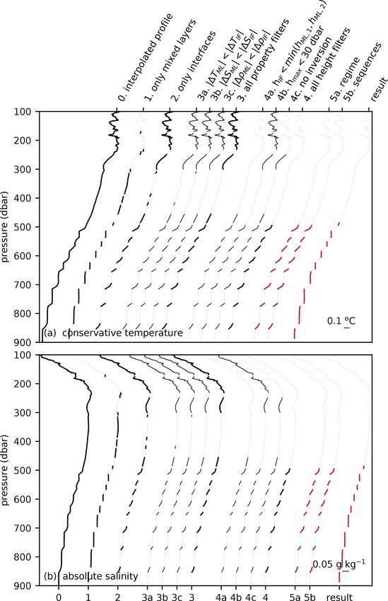
44                                                                         C. G. van der Boog et al.: Thermohaline staircases

Schmitt, 1981; Kelley, 1990; Radko and Smith, 2012; Ga-            Table 1. Number of floats and profiles in the global dataset. Profiles
raud, 2018). These results were confirmed by a tracer release      taken with Argo floats are categorized by the Data Assembly Centre
experiment in the western tropical Atlantic Ocean (Schmitt,        (DAC). Profiles taken with Ice-Tethered Profilers are categorized as
2005). Although these enhanced fluxes were observed, the           ITP. The percentage between brackets indicates the relative contri-
importance of these fluxes for the global mechanical energy        bution to the total number of profiles in the global dataset (487 493
                                                                   profiles). More details on abbreviations of DAC can be found in
budget remain unknown. Moreover, the vertical heat and salt
                                                                   Argo (2019).
fluxes in thermohaline staircases can also affect water-mass
properties. In some regions, persistent thermohaline stair-
                                                                           DAC/ITP       Number of floats               Profiles
cases with layers stretching over a few hundred kilometres
have been observed (Schmitt et al., 1987; Timmermans et al.,               aoml                      2692     312 285 (64.1 %)
2008; Shibley et al., 2017), which could result in significant             bodc                        93       11 092 (2.3 %)
diapycnal fluxes between water masses. For example, the                    coriolis                   347       27 134 (5.6 %)
double-diffusive diapycnal fluxes in the Mediterranean Sea                 csio                        81       15 099 (3.1 %)
                                                                           csiro                      378       42 942 (8.8 %)
dominate the transport between the deep water masses (Zo-
                                                                           incois                      65         4363 (0.9 %)
diatis and Gasparini, 1996; Bryden et al., 2014; Schroeder                 jma                        205       22 919 (4.7 %)
et al., 2016), and in the Arctic Ocean and Southern Ocean,                 kma                          1            1 (0.0 %)
an upward heat flux has been observed through staircase                    kordi                        0            0 (0.0 %)
interfaces (Timmermans et al., 2008; Shibley et al., 2017;                 meds                       145         9285 (1.9 %)
Polyakov et al., 2012; Bebieva and Speer, 2019).                           nmdis                        0            0 (0.0 %)
   Modelling studies that incorporated parameterizations of                ITP                         82       42 373 (8.7 %)
double-diffusive fluxes indicated that the associated double-
diffusive diapycnal fluxes can reduce the strength of the
global overturning circulation (Gargett and Holloway, 1992;        and Fig. 1, in which Fig. 1b confirms that all profiles have
Merryfield et al., 1999; Oschlies et al., 2003). To be able to     observations deeper than 500 dbar. Furthermore, the average
study this with observations, we present a global dataset of       vertical resolution of the profiles indicates the average reso-
the occurrence of thermohaline staircases and their proper-        lution is well below the 5 dbar that was used as a threshold
ties. The dataset is based on observations from Argo floats        (Fig. 1c). After this quality control, 487 493 vertical temper-
and Ice-Tethered Profilers. In the following sections we           ature and salinity profiles remain. Their global distribution is
briefly describe the raw data used to extract the dataset          shown in Fig. 2.
(Sect. 2) and the algorithm we designed to detect staircase           Next, the profiles of the Argo floats and ITP were linearly
structures (Sect. 3). The sensitivity of this detection algo-      interpolated to a vertical resolution of 1 dbar from the sur-
rithm to the chosen input parameters is assessed in Sect. 4.       face to 2000 dbar so that their data could be analysed in a
The dataset is verified in Sect. 5, followed by some guide-        consistent manner. As a result, the small steps in, for exam-
lines for the use of the dataset in Sect. 7.                       ple, Arctic staircases might be missed (see Sect. 5). From
                                                                   these interpolated profiles we calculate several variables. Ab-
                                                                   solute salinity (S) in grammes per kilogrammes and conser-
2    Data preparation                                              vative temperature (T ) in degrees Celsius are computed with
                                                                   the TEOS-10 software (McDougall and Barker, 2011). Note
The dataset contains observations of autonomous Argo floats        that we use conservative temperature as this is more accurate
and autonomous Ice-Tethered Profilers (ITPs). The data of all      than potential temperature in computations concerning heat
active and inactive profilers are obtained from http://www.        fluxes and heat content (Graham and McDougall, 2013). We
argo.ucsd.edu (last access: 14 May 2020) and http://www.           apply a moving average of 200 dbar (Table 2) to obtain the
whoi.edu/itp (last access: 14 May 2020) from 13 November           background conservative temperature and absolute salinity
2001 to 14 May 2020. Details on the profilers are described        profiles of the water column and to compute the thermal ex-
in Krishfield et al. (2008) and Toole et al. (2011) for the ITP    pansion coefficient (α, ◦ C−1 ) and the haline contraction co-
and in Argo (2020) for the Argo floats. First a quality check is   efficient (β, kg g−1 ). A consequence of the moving average
performed, where a profile is excluded from analysis if it was     of 200 dbar is that the upper 100 dbar and lower 100 dbar of
taken by an Argo float mentioned on the grey list. This grey       each profile are omitted in the remainder of the analysis. The
list contains floats that may have problems with at least one      Turner angle is computed using profiles that were smoothed
of the sensors (https://www.nodc.noaa.gov/argo/grey_floats.        with a moving average of 50 dbar instead of 200 dbar, which
htm, last access: 14 May 2020). As thermohaline staircases         is similar to Shibley et al. (2017), following Ruddick (1983),
consist of mixed layers with depths of tens of metres, we also     from
require that profiles have continuous data up to 500 dbar with
an average resolution finer than 5 dbar. Details on the origin
and vertical resolution of the profiles are depicted in Table 1

Earth Syst. Sci. Data, 13, 43–61, 2021                                                  https://doi.org/10.5194/essd-13-43-2021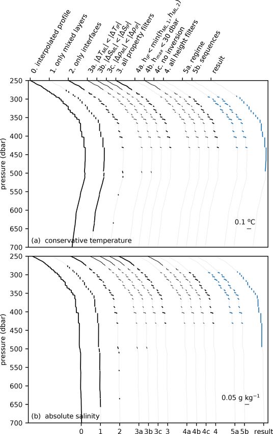
C. G. van der Boog et al.: Thermohaline staircases                                                                                           45

Figure 1. (a) Locations of observations categorized by Data Assembly Centres (DAC) when obtained by an Argo float. Profiles obtained
with Ice-Tethered Profilers are indicated with ITP. (b) Cumulative fraction of profiles that reached a given pressure in 25 dbar intervals from 0
to 2000 dbar per DAC. (c) Average number of observations in 25 dbar intervals from 0 to 2000 dbar. (d) Distribution of detected mixed-layer
pressures in the salt-finger (red histogram) or diffusive-convective (blue histogram) regime. (e) Number of detected mixed-layer height in the
salt-finger (red histogram) or diffusive-convective (blue histogram) regime. (f) Distribution of detected mixed-layer heights in thermohaline
staircases per pressure level. Panels (b, c) were obtained following Wong et al. (2020). Black lines indicate the averages in the total global
dataset. More details on abbreviations of DAC can be found in Argo (2019).

https://doi.org/10.5194/essd-13-43-2021                                                           Earth Syst. Sci. Data, 13, 43–61, 2021
46                                                                                C. G. van der Boog et al.: Thermohaline staircases

Figure 2. Observation density of the number of profiles obtained from the Argo floats and Ice-Tethered Profilers after quality control (km−2 ).
Observation density is binned per degree longitude and degree latitude. Empty bins indicate that no data were available at that location.

Table 2. Input parameters applied during the data preparation and the algorithm as used in this study. The sensitivity of the output of the
algorithm to the input variables is discussed in the Sect. 4.

                  Parameter                    Description                                                             Value
                  Moving average window        chosen to obtain background profiles                                200 dbar
                  ∂σ1 /∂pmax                   density gradient threshold for detection mixed layer   0.0005 kg m−3 dbar−1
                  1σ1,ML,max                   maximum density gradient within mixed layer                    0.005 kg m−3
                  hIF,max                      maximum interface height                                             30 dbar


                                                                                    −1         ∂T    ∂S ∂T    ∂S
                                                                          Tu = tan           α    − β ,α   +β      ,                       (1)
                                                                                               ∂p    ∂p ∂p    ∂p

                                                                          where the vertical gradients are approximated with a central
                                                                          differences scheme.

                                                                          3   Detection algorithm

                                                                          After the data pre-processing, we apply a detection algo-
                                                                          rithm that exploits the vertical structure of staircase profiles
                                                                          (Fig. 3). The benefit of using the vertical structure, instead
                                                                          of using assumptions based on the Turner angle, is that we
                                                                          can use this angle to verify the results. The detection algo-
                                                                          rithm consists of five steps. First the algorithm detects all
                                                                          data points that are located in the subsurface mixed lay-
Figure 3. Schematic of a typical temperature profile with staircases,     ers (ML, green dots in Fig. 3) by identifying weak vertical
indicating the definitions of the quantities used to detect the thermo-   density gradients in conservative temperature and absolute
haline staircases (green: mixed layer; orange: interface).                salinity. Next, the properties of any layer lying between the
                                                                          mixed layers (the interfaces, IF, orange dots in Fig. 3) are as-
                                                                          sessed by applying a minimum in temperature and salinity

Earth Syst. Sci. Data, 13, 43–61, 2021                                                          https://doi.org/10.5194/essd-13-43-2021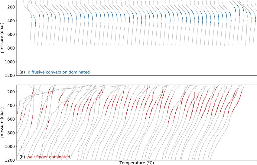
C. G. van der Boog et al.: Thermohaline staircases                                                                                          47

Figure 4. Histogram of the number of detected interfaces as a function of the Turner angle (Tu) by applying a criterion for (a) conservative
temperature, (b) absolute salinity, (c) potential density, and (d) all three properties given in Eq. (4) (orange shading). Each panel shows the
data remaining compared to the raw interface data (grey). Vertical shaded bands correspond to Turner angles in the diffusive-convective
(blue) and salt-finger (red) regimes.

variations. Third, the height of the interface and variations             ∂σ1 /∂pmax = 0.0005 kg m−3 dbar−1 (Table 2), which is sim-
within the interface are limited. The fourth step determines              ilar to mixed-layer gradients used by Bryden et al. (2014).
the regime of double diffusion (diffusive convection or salt              Furthermore, this threshold gradient is slightly larger than
fingers), and the fifth step is the identification of sequences           the threshold used by Timmermans et al. (2008), who
of interfaces, which eventually characterizes the thermoha-               used 0.005 ◦ C m−1 (which corresponds to ∂σ1 /∂pmax =
line staircases. The different steps of the algorithm applied to          0.00036 kg m−3 dbar−1 ). The threshold gradient method is
three example profiles are shown in Figs. A1–A3. In the fol-              applied to both conservative temperature and absolute salin-
lowing subsections, each algorithm step is described in more              ity profiles, i.e.,
detail.
                                                                               ∂T
                                                                           αρ0    ≤ 0.0005 kg m−3 dbar−1 ,
                                                                               ∂p
3.1   Mixed layers                                                             ∂S
                                                                           βρ0    ≤ 0.0005 kg m−3 dbar−1 .                                 (2)
                                                                               ∂p
The first step of the detection algorithm is the identification
of the mixed layers. Preferably, this is done by assessing a              Also the vertical density gradients from the combined tem-
density difference relative to a reference pressure, which is             perature and salinity effects must satisfy this condition:
the most reliable method to detect a mixed layer (Holte et al.,            ∂σ1
2017). However, in the case of a thermohaline staircase, it                    ≤ 0.0005 kg m−3 dbar−1 .                                    (3)
                                                                           ∂p
is necessary to detect subsurface mixed layers, because the
reference pressure is unknown beforehand. To determine this               These three conditions ensure that the vertical conservative
reference pressure, a threshold gradient criterion is applied             temperature, absolute salinity, and potential density gradi-
first (Dong et al., 2008). In this criterion, vertical density gra-       ents are all below the threshold value. At each pressure level
dients are identified as a mixed layer whenever the gradients             where all three conditions are met, the data point is identified
are below a certain threshold.                                            as a mixed layer. Next, for each continuous sequence of data
   We apply the gradient criterion to the vertical gra-                   points, the algorithm computes the average pressure. This is
dients of the potential density anomaly at a reference                    then used as a reference pressure, which is required to be able
pressure of 1000 dbar (σ1 ). We used a threshold of                       to apply the mixed-layer detection.

https://doi.org/10.5194/essd-13-43-2021                                                          Earth Syst. Sci. Data, 13, 43–61, 2021
48                                                                                 C. G. van der Boog et al.: Thermohaline staircases

Figure 5. Histogram of the number of detected interfaces as a function of the Turner angle (Tu) by applying a criteria for (a) height, (b)
maximum height, (c) inversions, and (d) all three height limitations (yellow shading). Each panel shows the data remaining compared to
the interfaces detected based on the conservative temperature and absolute salinity requirements shown in Fig. 4d (orange shading). Vertical
shaded bands correspond to Turner angles in the diffusive-convective (blue) and salt-finger (red) regimes.

Figure 6. Histogram of the number of detected interfaces as a function of the Turner angle (Tu) after (a) classification of the double-diffusive
regime and (b) selection of sequences of the interfaces. Each panel shows the data remaining compared to the interfaces detected based on
interface height requirement shown in Fig. 5d (yellow shading). Vertical shaded bands correspond to Turner angles in the diffusive-convective
(blue) and salt-finger (red) regimes.

   At every reference pressure, a maximum density range                   sity range corresponds to the density range used by Holte
is required within the mixed layers to identify the full ver-             et al. (2017) for the detection of surface mixed layers. The
tical extent of each mixed layer. To allow for small vari-                applied density range allows for mixed layers with heights
ations in conservative temperature and absolute salinity in               of the order of 10 m assuming gradients of ∂σ1 /∂pmax =
the mixed layer, but to exclude variations in the interface,              0.0005 kg m−3 dbar−1 . To ensure separation between individ-
we use a threshold of 1σ1,ML,max = 0.005 kg m−3 for den-                  ual mixed layers, the upper and lower data points of each
sity variations within each mixed layer (Table 2). This den-              mixed layer are removed. Note that this results in a mini-

Earth Syst. Sci. Data, 13, 43–61, 2021                                                         https://doi.org/10.5194/essd-13-43-2021
C. G. van der Boog et al.: Thermohaline staircases                                                                                      49

Figure 7. Example conservative temperature profiles selected by the staircase detection algorithm. They are ordered left to right by the
number of steps detected. Panel (a) shows examples of increasing steps of diffusive convection. Panel (b) shows examples of the salt-finger
regime.

Table 3. Characteristics of thermohaline staircases in Canada Basin. The region of the global dataset is confined to 75–80◦ N, 135–145◦ W.
The observational techniques indicate whether the data were obtained from Argo floats (Argo), Ice-Tethered Profilers (ITPs), conductivity–
temperature–depth (CTD) measurements, or microstructure measurements (MSs). The dominant type of thermohaline staircases is indicated
by DC (diffusive convection) and SF (salt-finger) with the percentage of occurrence between brackets. Ranges of the obtained variables of
the global dataset are indicated by means of percentiles 2.5 and 97.5.

                                          Technique            Type    Depth range            1TIF               1SIF      hIF
                                                                            (dbar)            (◦ C)          (g kg−1 )   (dbar)
           Global dataset                ITP + Argo      DC (90 %)         263–448       0.007–0.1        0.003–0.04       2–9
           Padman and Dillon (1987)        CTD+MS       DC (100 %)        320–430      0.004–0.013    0.0016–0.0049       0.15
           Timmermans et al. (2003)           CTD              DC       2400–2900      0.001–0.005    0.0035–0.0045       2–16
           Timmermans et al. (2008)            ITP       DC (96 %)        200–300              0.04            0.014
           Shibley et al. (2017)               ITP       DC (80 %)                      0.04 ± 0.01     0.01 ± 0.003     < 1m

mum interface height of 2 dbar, which could result in false             erage Turner angle (TuML ), and height (hML ) for each mixed
negatives in for example the Arctic Ocean (Sect. 5)                     layer.
   After applying the threshold for density range, the algo-
rithm defines each continuous set of data points as a mixed             3.2   Interfaces: conservative temperature and absolute
layer and computes the average pressure (p ML ), average                      salinity variations
conservative temperature (T ML ), average absolute
                                                    salinity

                                           ∂T     ∂S
(S ML ), mixed-layer density ratio R ρ = α ∂p / β ∂p , av-              The algorithm defines an interface as the part of the water
                                                                        column between two mixed layers. In addition, to ensure a

https://doi.org/10.5194/essd-13-43-2021                                                       Earth Syst. Sci. Data, 13, 43–61, 2021
50                                                                                  C. G. van der Boog et al.: Thermohaline staircases

Figure 8. Number of detected interfaces obtained with the detection algorithm for different input parameters. Each panel shows the sensitivity
of the detection algorithm to one input parameter: (a) moving average window, (b) density gradient of the mixed layer, (c) density difference
within the mixed layer, and (d) the maximum height of the interface. In each panel, the grey histogram corresponds to the default parameters
listed in Table 2. The coloured lines correspond to the varying parameter (see legend). Shaded regions indicate Turner angles in the diffusive-
convective (blue) and salt-finger (red) regimes.

Table 4. As Table 3, but for the Mediterranean Sea (30–43◦ N, 0–15◦ E).

                                                 Technique           Type     Depth range             1TIF             1SIF      hIF
                                                                                   (dbar)             (◦ C)        (g kg−1 )   (dbar)
         Global dataset                         ITP + Argo       SF (6 %)          287–866   0.0097–0.12      0.0017–0.031      3–21
         Zodiatis and Gasparini (1996)                CTD             SF          600–2500      0.04–0.17        0.01–0.04      2–27
         Bryden et al. (2014)                         CTD      SF (32 %)          600–1400      0.03–0.13       0.009–0.03      5–16
         Buffett et al. (2017)             seismic imaging            SF          550–1200
         Durante et al. (2019)                        CTD             SF          500–2500   approx. 0.15                       4–17

stepped structure, the algorithm requires that the conserva-                in the interfaces on the Turner angle is in line with expec-
tive temperature, absolute salinity, and potential density vari-            tations that staircase-like structures are mostly found within
ations within each mixed layer should be smaller than the                   double-diffusive regimes. In total, 28 % of all detected inter-
variations in the interface (Fig. 3):                                       faces meet all three requirements (Fig. 4d).

max 1TML,1 , 1TML,2 < |1TIF | ;

max 1SML,1 , 1SML,2 < |1SIF | ;                                             3.3   Interface: height

max 1σ1,ML,1 , 1σ1,ML,2 < 1σ1,IF ;                          (4)
                                                                            The next step in the staircase detection algorithm is to limit
where the subscripts 1 and 2 correspond to the mixed layer                  the height of the interface to ensure that the mixed layers
directly above and below an interface, respectively. It ap-                 are separated from each other by a relatively thin interface
pears that most data points that meet these requirements (or-               (Fig. 3). We require
ange histograms in Fig. 4a–c) have Turner angles in the two
double-diffusive regimes. This dependence of the variations                 hIF < min hML,1 , hML,2 ;                                      (5)

Earth Syst. Sci. Data, 13, 43–61, 2021                                                         https://doi.org/10.5194/essd-13-43-2021
C. G. van der Boog et al.: Thermohaline staircases 51
Table 5. As Table 3, but for the western tropical North Atlantic Ocean (10–15◦ N, 53–58◦ W).
Technique Type Depth range 1TIF 1SIF hIF
(dbar) (◦ C) (g kg−1 ) (dbar)
Global dataset ITP + Argo SF (60 %) 265–837 0.019–0.97 0.0014–0.16 3–18
Schmitt et al. (1987) CTD+MSs SF 180–650 0.5–0.8 0.1–0.2 psu 1–10
Schmitt (2005) CTD+MSs SF 200–60052 C. G. van der Boog et al.: Thermohaline staircases
cation were weak enough (see Sect. 3.1). Furthermore, both faces remain confined to the two double-diffusive regimes,
conservative temperature and absolute salinity in this mixed indicating a robust outcome of the algorithm for the choice
layer are larger than in the mixed layer above. While both of this input parameter.
are typical for a staircase in the diffusive-convective regime, Similar to the variations in the maximum density gra-
the algorithm does not detect whether this mixed layer is dient, the variation in the maximum density difference al-
a temperature maximum, which could indicate that it arose lowed within the mixed-layer results in a different num-
from thermohaline intrusions. Note that this only concerns ber of detected interfaces (Fig. 8c). The number of detected
the deepest mixed layers of the staircases and that only the mixed layers increases when we decrease the maximum den-
characteristics of the interfaces in between mixed layers are sity difference allowed within the mixed layer. This effect
labelled as part of a staircase by the algorithm. is mostly visible in the diffusive-convective regime, as we
Thermohaline staircases with a high number of steps in obtained a decrease of 54 % of detected interfaces in the
the salt-finger regime are detected on the main thermo- diffusive-convective regime compared to a decrease of 31 %
cline where the conservative temperature decreases with of detected interfaces in the salt-finger regime in the case in
depth (Fig. 7b). Compared to the staircases in the diffusive- which we doubled the density difference in the mixed layer
convective regime, these staircases are located slightly (1σ1,max = 10 × 10−3 kg m−3 ). This difference between the
deeper at 400–700 m. While the locations of these staircases regimes is due to relatively small interface variations in
vary, they are located above the cold and fresh Antarctic In- the diffusive-convective regime compared to the salt-finger
termediate Water, which is observed below 700 m (Tsuchiya, regime (Radko, 2013) and can be explained as follows: when
1989; Fine, 1993; Talley, 1996). a too large density difference is applied, the relatively small
For each thermohaline staircase, characteristics of the in- density gradients in the interfaces of the diffusive-convective
terfaces and mixed layers, such as their conservative tem- regime are detected as mixed layers by the algorithm. Con-
perature, absolute salinity, and height, are available in the sequently, multiple mixed layers can be identified as a single
dataset. An overview of the provided variables is given in Ta- mixed layer. However, if the applied density difference is too
ble A1. The detection algorithm is verified by comparing our small, this could result in the detection of multiple mixed
data to independent observations in three regions in Sect. 5. layers per staircase step.
The last input parameter of the detection algorithm con-
cerns the interface height (Fig. 8d). As expected from Fig. 5b,
4 Robustness of the detection algorithm variations in this input parameter do not result in large differ-
ences in the number of detected interfaces. If we omit this
The algorithm requires four input parameters: the moving input parameter by setting it to infinity, we obtain a total in-
average window, a threshold for the maximum density gra- crease in detected interfaces of 17 %.
dients of the mixed layers, the maximum density difference Overall, the detection algorithm gives robust results as it
of the mixed layers, and the maximum height of the interface predominantly detects interfaces within the double-diffusive
(Table 2). In this section, the sensitivity of the algorithm to regime (Fig. 8). In line with expectations, the detection algo-
each input parameter is assessed (Fig. 8). rithm is most sensitive to the threshold value for the max-
The moving average window is used by the algorithm imum density gradient in the mixed layer and the density
to compute the thermal expansion coefficient (α), the ha- variations within the mixed layers. The four input variables
line contraction coefficient (β), and the density ratio (Rρ ). allow for optimization of the detection algorithm based on
We varied the moving average window between 50 and the regime and characteristics of the staircases.
350 dbar to assess the sensitivity of the outcomes of this
choice (Fig. 8a). We find that the varying moving average
window does not result in large variations in detected mixed 5 Regional verification
layers (Fig. 8a).
In contrast to the moving-average window, the detection The characteristics of thermohaline staircases obtained with
algorithm is sensitive to the value set for the density gradi- the detection algorithm are compared to those obtained from
ent threshold of the mixed layer (Fig. 8b), which is used to previous observational studies for three major staircase re-
obtain a reference pressure for the sub-surface mixed lay- gions: the Canada Basin in the Arctic Ocean, the Mediter-
ers (Sect. 3.1). Not surprisingly, we detect more (fewer) in- ranean Sea, and the C-SALT region in the tropical Atlantic
terfaces when we increase (decrease) the allowed threshold Ocean. An overview is given in Tables 3–5.
density gradient. A small value allows for only the strongest In the Canada Basin (75–80◦ N, 135–145◦ W), the al-
mixed layers to be detected, which are usually referred to as gorithm detects thermohaline staircases in the diffusive-
well-defined staircases, while a large density gradient also al- convective regime in 90 % of the profiles (Table 3). Both
lows for the detection of rough staircases (e.g., Durante et al., the occurrence and depth range are comparable to what was
2019). Although the number of detected interfaces depends reported by Timmermans et al. (2008) and Shibley et al.
on the value set for this density gradient, the detected inter- (2017), who analysed thermohaline staircases from several
Earth Syst. Sci. Data, 13, 43–61, 2021 https://doi.org/10.5194/essd-13-43-2021C. G. van der Boog et al.: Thermohaline staircases 53
Ice-Tethered Profilers, demonstrating that our detection al- vertical resolution and the limitation imposed by the detec-
gorithm indeed detects thermohaline staircases at the right tion algorithm to avoid detection of false positives. Despite
location. Microstructure observations suggested that the ther- this overestimation, the interfaces are detected at the correct
mohaline staircases in Canada Basin have interface heights depths with conservative temperature and absolute salinity
of approximately hIF = 0.15 m (Padman and Dillon, 1987; steps within realistic ranges. Therefore, we conclude that the
Radko, 2013). Due to the vertical resolution of the profiles detection algorithm is very suitable for the automated detec-
and the design of the algorithm (recall that the mixed lay- tion of thermohaline staircases in large and quickly growing
ers are separated from each other by removing the upper and datasets like the Argo float and Ice-Tethered-Profiler data.
lower data points of the mixed layer, Sect. 3.1), the method
is not capable of detecting very thin interfaces (Fig. A1). As
6 Code and data availability
expected from these limitations for the detection of the in-
terface heights, the algorithm detects conservative temper-
Both algorithm and global dataset are available at DOI:
ature and absolute salinity steps (1TIF and 1SIF , respec-
https://doi.org/10.5281/zenodo.4286170 (van der Boog et al.,
tively) in the interfaces that are in the upper ranges of ear-
2020). The algorithm is written in Python 3 and is available
lier observations (Padman and Dillon, 1987; Timmermans
under the Creative Commons Attribution 4.0 License. More
et al., 2003, 2008; Shibley et al., 2017). In the Mediterranean
details on the functions and output of the algorithm are de-
Sea, thermohaline staircases are characterized by relatively
picted in Tables A1 and A2, respectively. The structure of the
thick mixed layers that are separated by thick interfaces of
algorithm is displayed in Fig. A4. The Argo Program is part
up to 27 m (Zodiatis and Gasparini, 1996). In this region
of the Global Ocean Observing System (Argo, 2020).
(30–43◦ N, 0–15◦ E), the detection algorithm detected ther-
mohaline staircases with interfaces up to 21 dbar in 6 % of
the profiles, which is comparable to previous observations 7 Conclusions
(Table 4). An example of the detection of a Mediterranean
staircase is shown in Fig. A2. We find that the depth at which In this study, we presented an algorithm to automatically de-
the thermohaline staircases occur is underestimated by the tect thermohaline staircases from Argo float profiles and Ice-
detection algorithm. This could be explained by the fact that Tethered Profiles. As these thermohaline staircases have dif-
most Mediterranean observations are obtained by the Cori- ferent mixed-layer heights and temperature and salinity steps
olis DAC (Fig. 1a). From this DAC, approximately 50 % of across the interfaces in different staircase regions, the design
the profiles have observations that are deeper than 1000 dbar of the detection algorithm is based on the typical vertical
(Fig. 1b), which means that the coverage below 1000 dbar is structure and shape of the staircases (Figs. 3–5). Note that
limited in the Mediterranean Sea. Although the Argo floats, by formulating the algorithm solely on this vertical struc-
and consequently the detection algorithm, do not cover the ture of the staircases, we could use the Turner angle of the
full extent of the staircases (Fig. 1), the conservative temper- detected staircases for verification. Using this Turner angle,
ature and absolute salinity steps that are found are similar to we showed that the structures are within the two double-
previous observations (Table 4). Note that the conservative diffusive regimes: the salt-finger regime and the diffusive-
temperature and absolute salinity steps of the staircases in- convective regime (Fig. 6).
crease with depth (Zodiatis and Gasparini, 1996), which ex- We optimized the input of the algorithm such that it
plains why the conservative temperature and absolute salinity provides a global overview and limits the number of de-
steps detected by the algorithm are slightly smaller than those tected false positives. As a result, the regional verification in
observed in the deeper observations (Zodiatis and Gasparini, Sect. 5 indicated that the data pre-processing and data anal-
1996; Durante et al., 2019). ysis have some limitations. For example, the vertical reso-
In the C-SALT region in the western tropical North At- lution of 1 dbar in the profiles is too course to capture all
lantic Ocean (10–15◦ N, 53–58◦ W), the algorithm detected staircase steps in the Arctic Ocean. In the Mediterranean,
thermohaline staircases in the salt-finger regime in 60 % of the Argo floats did not dive deep enough to capture the full
the profiles (Table 5). Similar to previous studies (Schmitt depth of the staircase region. However, the fact that (i) the
et al., 1987; Schmitt, 2005; Fer et al., 2010), the algorithm algorithm detects thermohaline staircases at realistic depth
detected thermohaline staircases on the main thermocline ranges, with (ii) conservative temperature and absolute salin-
(see example in Fig. A3). Again, the interface height is ity steps across the interfaces, and in (iii) the same double-
slightly overestimated by the detection algorithm, but the diffusive regime as previous studies (Tables 3–5), indicates
algorithm obtained conservative temperature and absolute that the algorithm itself performs well. Therefore, when con-
salinity steps comparable to previous studies. sidering an individual staircase region, we recommend opti-
Overall, the comparison between the outcomes of the de- mizing the input variables of the algorithm for that specific
tection algorithm with previous studies indicates that the region and applying the algorithm to additional data, for ex-
detection algorithm performs well. The small overestima- ample high-resolution CTD or microstructure profiles, where
tion of the interface height can be attributed to the limited available.
https://doi.org/10.5194/essd-13-43-2021 Earth Syst. Sci. Data, 13, 43–61, 202154 C. G. van der Boog et al.: Thermohaline staircases A sensitivity analysis to different input parameters showed The global dataset resulting from the detection algorithm that the results of the detection algorithm are robust; the contains properties and characteristics of both mixed layers detected staircase interfaces are confined to the double- and interfaces. Combined with their locations, these data al- diffusive regimes. Furthermore, the comparison between the low for a statistical analysis of thermohaline staircases on detected interface characteristics of thermohaline staircases global scales. For example, the global occurrence of ther- in three prevailing staircase regions and previous observa- mohaline staircases could give insight into the contribution tions suggested that the detection algorithm accurately cap- of double diffusion to the global mechanical energy budget. tures both double-diffusive regimes. The algorithm detected Moreover, the interface characteristics can be used to vali- correct magnitudes of the conservative temperature and ab- date model and laboratory results on how double-diffusive solute salinity steps in the interfaces, which allows for ad- mixing impacts the regional ocean circulation. equate estimates of the effective diffusivity in thermohaline staircases. Earth Syst. Sci. Data, 13, 43–61, 2021 https://doi.org/10.5194/essd-13-43-2021
C. G. van der Boog et al.: Thermohaline staircases                                                                                       55

Appendix A

Figure A1. Steps of the detection algorithm applied to a profile in the Arctic Ocean, where steps are indicated on separate (a) conservative
temperature and (b) absolute salinity profiles. Each profile is shifted for clarity. Similar to Figs. 4–6, an interface is not considered by
the detection algorithm when the interface characteristics did not meet the requirements of a previous step. Original profile is taken from
Ice-Tethered Profiler ITP64 at 137.8◦ W and 75.2◦ N on 29 January 2013. The details of the data preparation and the algorithm steps are
discussed in Sects. 2 and 3, respectively.

https://doi.org/10.5194/essd-13-43-2021                                                       Earth Syst. Sci. Data, 13, 43–61, 2021
56                                                                             C. G. van der Boog et al.: Thermohaline staircases

Figure A2. As Fig. A1, but for a profile in the Mediterranean Sea. Original profile is taken from Argo float 6901769 at 8.9◦ E and 37.9◦ N
on 31 October 2017.

Earth Syst. Sci. Data, 13, 43–61, 2021                                                     https://doi.org/10.5194/essd-13-43-2021
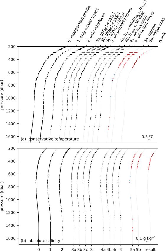
C. G. van der Boog et al.: Thermohaline staircases                                                                                          57

Figure A3. As Fig. A1, but for a profile in the western tropical North Atlantic. Original profile is taken from Argo float 4 901 478 at 53.3◦ W
and 11.6◦ N on 9 August 2014.

https://doi.org/10.5194/essd-13-43-2021                                                          Earth Syst. Sci. Data, 13, 43–61, 2021
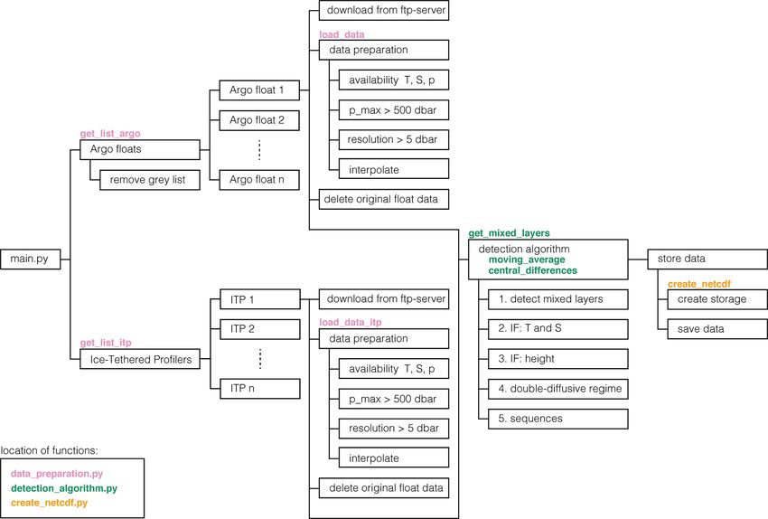
58                                                                               C. G. van der Boog et al.: Thermohaline staircases

Figure A4. Structure of the software. Each step in the software is shown by a box. Whenever a particular step is contained inside a function,
the name of the function is mentioned above the step. Details of the preprocessing of the data and the detection algorithm are discussed in
Sects. 2 and 3, respectively.

Table A1. Metadata of all variables that are saved in the dataset.

                              Variable    Unit      Description
                              floatID               float identification number of ITP or Argo float
                              lat         ◦E        latitude of observation
                              lon         ◦N        longitude of observation
                              juld        d         Julian date of observation
                              ct          ◦C        conservative temperature (full profile)
                              sa          g kg−1    absolute salinity (full profile)
                              MLSF                  mask with mixed layers in the salt-finger regime
                              MLDC                  mask with mixed layers in the diffusive-convective regime
                              pML         dbar      average pressure of the mixed layer
                              hML         dbar      height of the mixed layer
                              TML         ◦C        average conservative temperature of mixed layer
                              SML         g kg−1    average absolute salinity of mixed layer
                              TuML        ◦         average Turner angle of mixed layer
                              RML                   average density ratio of the mixed layer
                              hIF         dbar      height of the interface
                              TuIF        ◦         Turner angle at the centre of the interface
                              RIF                   density ratio at the centre of the interface
                              1TIF        ◦C        conservative temperature difference within the interface
                              1SIF        g kg−1    absolute salinity difference within the interface

Earth Syst. Sci. Data, 13, 43–61, 2021                                                        https://doi.org/10.5194/essd-13-43-2021
C. G. van der Boog et al.: Thermohaline staircases 59
Table A2. Functions used in the software.
Function Input Output Description
get_list_argo centers, filename directory, floats, float_list Access FTP server (ftp://ftp.ifremer.fr, last ac-
cess: 14 May 2020) and navigate through direc-
tories of the Data Assembly Centres (centers)
to locate the Argo floats from the input list (file-
name). Directory of floats on the FTP server are
given in directory. The full list of Argo floats
before removal of the floats of the grey list is
given in floats. Argo floats mentioned on the
grey list are removed. Required packages are ft-
plib, numpy, and pandas.
get_list_itp – list of floats Access FTP server (ftp://ftp.whoi.edu, last ac-
cess: 14 May 2020) to obtain list of available
Ice-Tethered Profilers. Required packages are
ftplib and numpy.
load_data filename, interp p, lat, lon, ct, sa, juld The profiles of a single Argo float (filename) are
evaluated and linearly interpolated to a resolu-
tion of 1 dbar (interp=True). Only profiles with
an average resolution finer than 5 dbar and pres-
sure levels exceeding 500 dbar are considered.
Output contains interpolated data of pressure,
latitude (lat), longitude (lat), conservative tem-
perature (ct), absolute salinity (sa), and Julian
date (juld). Required packages are gsw, numpy,
netCDF4, and scipy.
load_data_itp path,profiles,interp prof_no, p, lat, lon, ct, sa, juld Similar to load_data, but then for Ice-Tethered
Profilers. There is an additional output contain-
ing the FloatID of the ITP (prof_no). Required
packages are datetime, gsw, numpy, pandas, and
scipy.
get_mixed_layers p, ct, sa, c1, c2, c3, c4 ml, gl, masks This is the detection algorithm. Input contains
the pressure, conservative temperature, abso-
lute salinity, and user-defined input parameters:
∂σ1 /∂pmax (c1), 1σ1,ML,max (c2), moving av-
erage window (c4), hIF,max (c3). The output
is classes with the mixed-layer characteristics
(ml), interface characteristics (gl), and masks
(see details in Table A1). Required packages are
gsw, numpy, and scipy.
moving_average2d dataset, window mav Apply moving average window (window) to
vertical profiles (dataset) and obtain back-
ground profiles (mav). Required packages are
numpy and scipy.
central_differences2d f, z dfdz Compute vertical gradients with central differ-
ences scheme. The required packages is numpy.
https://doi.org/10.5194/essd-13-43-2021 Earth Syst. Sci. Data, 13, 43–61, 202160 C. G. van der Boog et al.: Thermohaline staircases
Author contributions. CvdB and JOK designed the detection Fer, I., Nandi, P., Holbrook, W. S., Schmitt, R. W., and
scheme. CvdB wrote the paper and was supervised by CAK, JDP, Páramo, P.: Seismic imaging of a thermohaline staircase in
and HAD, who helped shape the analysis and paper. the western tropical North Atlantic, Ocean Sci., 6, 621–631,
https://doi.org/10.5194/os-6-621-2010, 2010. Fer, I., Nandi, P.,
Holbrook, W. S., Schmitt, R. W., and Páramo, P.: Seismic Imag-
Competing interests. The authors declare that they have no con- ing of a Thermohaline Staircase in the Western Tropical North
flict of interest. Atlantic, Ocean Sci., 6, 621–631, https://doi.org/10.5194/os-6-
621-2010, 2010.
Fine, R. A.: Circulation of Antarctic Intermediate Water in the
Acknowledgements. The Ice-Tethered Profiler data were col- South Indian Ocean, Deep-Sea Res. Pt. I, 40, 2021–2042,
lected and made available by the Ice-Tethered Profiler Program https://doi.org/10.1016/0967-0637(93)90043-3, 1993.
(Krishfield et al., 2008; Toole et al., 2011) based at Woods Hole Garaud, P.: Double-Diffusive Convection at Low Prandtl
Oceanographic Institution (http://www.whoi.edu/itp, last access: 14 Number, Annu. Rev. Fluid Mech., 50, 275–298,
May 2020). The Argo data were collected and made freely available https://doi.org/10.1146/annurev-fluid-122316-045234, 2018.
by the International Argo Program and the national programmes Gargett, A. E. and Holloway, G.: Sensitivity of the GFDL
that contribute to it (http://www.argo.ucsd.edu, last access: 16 July Ocean Model to Different Diffusivities for Heat and Salt, J.
2020, http://argo.jcommops.org, last access: 16 July 2020). Phys. Oceanogr., 22, 1158–1177, https://doi.org/10.1175/1520-
0485(1992)0222.0.CO;2, 1992.
Graham, F. S. and McDougall, T. J.: Quantifying the Noncon-
servative Production of Conservative Temperature, Potential
Financial support. This research has been supported by the Delft
Temperature, and Entropy, J. Phys. Oceanogr., 43, 838–862,
University of Technology Delft Technology Fellowship awarded to
https://doi.org/10.1175/JPO-D-11-0188.1, 2013.
Caroline A. Katsman.
Holte, J., Talley, L. D., Gilson, J., and Roemmich, D.: An Argo
Mixed Layer Climatology and Database, Geophys. Res. Lett., 44,
5618–5626, https://doi.org/10.1002/2017GL073426, 2017.
Review statement. This paper was edited by Giuseppe Kelley, D. E.: Fluxes through Diffusive Staircases:
M. R. Manzella and reviewed by three anonymous referees. A New Formulation, J. Geophys. Res., 95, 3365,
https://doi.org/10.1029/JC095iC03p03365, 1990.
Krishfield, R., Toole, J., Proshutinsky, A., and Timmermans, M.-
References L.: Automated Ice-Tethered Profilers for Seawater Observations
under Pack Ice in All Seasons, J. Atmos. Ocean. Tech., 25, 2091–
Argo: Argo User’s Manual V3.3, Ifremer, Brest, France, 2105, https://doi.org/10.1175/2008JTECHO587.1, 2008.
https://doi.org/10.13155/29825, 2019. McDougall, T. J. and Barker, P. M.: Getting Started with TEOS-
Argo: Argo Float Data and Metadata from Global 10 and the Gibbs Seawater (GSW) Oceanographic Toolbox,
Data Assembly Centre (Argo GDAC), SEANOE, SCOR/IAPSO WG, 127, 1–28, 2011.
https://doi.org/10.17882/42182, 2020. Merryfield, W. J.: Origin of Thermohaline Staircases, J. Phys.
Bebieva, Y. and Speer, K.: The Regulation of Sea Ice Oceanogr., 30, 1046–1068, https://doi.org/10.1175/1520-
Thickness by Double-Diffusive Processes in the Ross 0485(2000)0302.0.CO;2, 2000.
Gyre, J. Geophys. Res.-Oceans, 124, 7068–7081, Merryfield, W. J., Holloway, G., and Gargett, A. E.: A
https://doi.org/10.1029/2019JC015247, 2019. Global Ocean Model with Double-Diffusive Mixing, J.
Bebieva, Y. and Timmermans, M.-L.: The Relationship between Phys. Oceanogr., 29, 1124–1142, https://doi.org/10.1175/1520-
Double-Diffusive Intrusions and Staircases in the Arctic Ocean, 0485(1999)0292.0.CO;2, 1999.
J. Phys. Oceanogr., 47, 867–878, https://doi.org/10.1175/JPO-D- Oschlies, A., Dietze, H., and Kähler, P.: Salt-Finger Driven En-
16-0265.1, 2017. hancement of Upper Ocean Nutrient Supply, Geophys. Res. Lett.,
Bryden, H. L., Schroeder, K., Sparnocchia, S., Borgh- 30, https://doi.org/10.1029/2003GL018552, 2003.
ini, M., and Vetrano, A.: Thermohaline Staircases in Padman, L. and Dillon, T. M.: Vertical Heat Fluxes through the
the Western Mediterranean Sea, J. Mar. Res., 72, 1–18, Beaufort Sea Thermohaline Staircase, J. Geophys. Res., 92,
https://doi.org/10.1357/002224014812655198, 2014. 10799, https://doi.org/10.1029/JC092iC10p10799, 1987.
Buffett, G. G., Krahmann, G., Klaeschen, D., Schroeder, K., Sal- Polyakov, I. V., Pnyushkov, A. V., Rember, R., Ivanov, V. V.,
larès, V., Papenberg, C., Ranero, C. R., and Zitellini, N.: Seis- Lenn, Y.-D., Padman, L., and Carmack, E. C.: Mooring-
mic Oceanography in the Tyrrhenian Sea: Thermohaline Stair- Based Observations of Double-Diffusive Staircases over
cases, Eddies, and Internal Waves, J. Geophys. Res.-Oceans, 122, the Laptev Sea Slope, J. Phys. Oceanogr., 42, 95–109,
8503–8523, https://doi.org/10.1002/2017JC012726, 2017. https://doi.org/10.1175/2011JPO4606.1, 2012.
Dong, S., Sprintall, J., Gille, S. T., and Talley, L.: Southern Ocean Radko, T.: A Mechanism for Layer Formation in a
Mixed-Layer Depth from Argo Float Profiles, J. Geophys. Res., Double-Diffusive Fluid, J. Fluid Mech., 497, 365–380,
113, C06013, https://doi.org/10.1029/2006JC004051, 2008. https://doi.org/10.1017/S0022112003006785, 2003.
Durante, S., Schroeder, K., Mazzei, L., Pierini, S., Borghini, M., Radko, T.: Double-Diffusive Convection, Cambridge University
and Sparnocchia, S.: Permanent Thermohaline Staircases in Press, Cambridge, https://doi.org/10.1017/CBO9781139034173,
the Tyrrhenian Sea, Geophys. Res. Lett., 46, 1562–1570, 2013.
https://doi.org/10.1029/2018GL081747, 2019.
Earth Syst. Sci. Data, 13, 43–61, 2021 https://doi.org/10.5194/essd-13-43-2021C. G. van der Boog et al.: Thermohaline staircases 61 Radko, T. and Smith, D. P.: Equilibrium Transport in Timmermans, M.-L., Toole, J., Krishfield, R., and Winsor, P.: Ice- Double-Diffusive Convection, J. Fluid Mech., 692, 5–27, Tethered Profiler Observations of the Double-Diffusive Stair- https://doi.org/10.1017/jfm.2011.343, 2012. case in the Canada Basin Thermocline, J. Geophys. Res., 113, Ruddick, B.: A Practical Indicator of the Stability of the Water C00A02, https://doi.org/10.1029/2008JC004829, 2008. Column to Double-Diffusive Activity, Deep-Sea Res., 30, 1105– Toole, J. M., Krishfield, R., Timmermans, M.-L., and Proshutin- 1107, https://doi.org/10.1016/0198-0149(83)90063-8, 1983. sky, A.: The Ice-Tethered Profiler: Argo of the Arctic, Oceanog- Ruddick, B. and Kerr, O.: Oceanic Thermohaline Intru- raphy, 24, 126–135, 2011. sions: Theory, Double-Diffus. Oceanogr., 56, 483–497, Tsuchiya, M.: Circulation of the Antarctic Intermediate Wa- https://doi.org/10.1016/S0079-6611(03)00029-6, 2003. ter in the North Atlantic Ocean, J. Mar. Res., 47, 747–755, Rudels, B.: Arctic Ocean Circulation, Processes and Wa- https://doi.org/10.1357/002224089785076136, 1989. ter Masses: A Description of Observations and Ideas van der Boog, C. G., Koetsier, J. O., Dijkstra, H. A., with Focus on the Period Prior to the International Po- Pietrzak, J. D., and Katsman, C. A.: Data Supplement for lar Year 2007–2009, Progr. Oceanogr., 132, 22–67, ‘Global Dataset of Thermohaline Staircases Obtained from Argo https://doi.org/10.1016/j.pocean.2013.11.006, 2015. Floats and Ice-Tethered Profilers’ (Version 1), Data set, Zenodo, Schmitt, R., Perkins, H., Boyd, J., and Stalcup, M.: C-SALT: https://doi.org/10.5281/ZENODO.4286170, 2020. An Investigation of the Thermohaline Staircase in the Western Wong, A. P. S., Wijffels, S. E., Riser, S. C., Pouliquen, S., Tropical North Atlantic, Pt. I, Deep-Sea Res., 34, 1655–1665, Hosoda, S., Roemmich, D., Gilson, J., Johnson, G. C., Mar- https://doi.org/10.1016/0198-0149(87)90014-8, 1987. tini, K., Murphy, D. J., Scanderbeg, M., Bhaskar, T. V. S. U., Schmitt, R. W.: Form of the Temperature-Salinity Relationship in Buck, J. J. H., Merceur, F., Carval, T., Maze, G., Cabanes, C., the Central Water: Evidence for Double-Diffusive Mixing, J. André, X., Poffa, N., Yashayaev, I., Barker, P. M., Guinehut, S., Phys. Oceanogr., 11, 1015–1026, https://doi.org/10.1175/1520- Belbéoch, M., Ignaszewski, M., Baringer, M. O., Schmid, C., 0485(1981)0112.0.CO;2, 1981. Lyman, J. M., McTaggart, K. E., Purkey, S. G., Zilberman, N., Schmitt, R. W.: Double Diffusion in Oceanog- Alkire, M. B., Swift, D., Owens, W. B., Jayne, S. R., Hersh, C., raphy, Annu. Rev. Fluid Mech., 26, 255–285, Robbins, P., West-Mack, D., Bahr, F., Yoshida, S., Sutton, P. J. H., https://doi.org/10.1146/annurev.fl.26.010194.001351, 1994. Cancouët, R., Coatanoan, C., Dobbler, D., Juan, A. G., Gour- Schmitt, R. W.: Enhanced Diapycnal Mixing by Salt Fingers in the rion, J., Kolodziejczyk, N., Bernard, V., Bourlès, B., Claus- Thermocline of the Tropical Atlantic, Science, 308, 685–688, tre, H., D’Ortenzio, F., Le Reste, S., Le Traon, P.-Y., Ran- https://doi.org/10.1126/science.1108678, 2005. nou, J.-P., Saout-Grit, C., Speich, S., Thierry, V., Verbrugge, N., Schroeder, K., Chiggiato, J., Bryden, H. L., Borgh- Angel-Benavides, I. M., Klein, B., Notarstefano, G., Poulain, P.- ini, M., and Ben Ismail, S.: Abrupt Climate Shift in M., Vélez-Belchí, P., Suga, T., Ando, K., Iwasaska, N., the Western Mediterranean Sea, Sci. Rep.-UK, 6, 23009, Kobayashi, T., Masuda, S., Oka, E., Sato, K., Nakamura, T., https://doi.org/10.1038/srep23009, 2016. Sato, K., Takatsuki, Y., Yoshida, T., Cowley, R., Lovell, J. L., Shibley, N. C., Timmermans, M.-L., Carpenter, J. R., and Oke, P. R., van Wijk, E. M., Carse, F., Donnelly, M., Gould, W. J., Toole, J. M.: Spatial Variability of the Arctic Ocean’s Double- Gowers, K., King, B. A., Loch, S. G., Mowat, M., Turton, J., Diffusive Staircase, J. Geophys. Res.-Oceans, 122, 980–994, Rama Rao, E. P., Ravichandran, M., Freeland, H. J., Gaboury, I., https://doi.org/10.1002/2016JC012419, 2017. Gilbert, D., Greenan, B. J. W., Ouellet, M., Ross, T., Tran, A., Stern, M. E.: The “Salt-Fountain” and Thermohaline Convection, Dong, M., Liu, Z., Xu, J., Kang, K., Jo, H., Kim, S.-D., and Tellus, 12, 172–175, https://doi.org/10.3402/tellusa.v12i2.9378, Park, H.-M.: Argo Data 1999–2019: Two Million Temperature- 1960. Salinity Profiles and Subsurface Velocity Observations From a Stern, M. E.: Collective Instability of Salt Fingers, J. Fluid Mech., Global Array of Profiling Floats, Frontiers in Marine Science, 7, 35, 209–218, https://doi.org/10.1017/S0022112069001066, 700, https://doi.org/10.3389/fmars.2020.00700, 2020. 1969. Zodiatis, G. and Gasparini, G. P.: Thermohaline Staircase Forma- Talley, L. D.: Antarctic Intermediate Water in the South tions in the Tyrrhenian Sea, Deep-Sea Res. Pt. I, 43, 655–678, Atlantic, pp. 219–238, Springer, Berlin, Heidelberg, https://doi.org/10.1016/0967-0637(96)00032-5, 1996. https://doi.org/10.1007/978-3-642-80353-6_11, 1996. Timmermans, M.-L., Garrett, C., and Carmack, E.: The Ther- mohaline Structure and Evolution of the Deep Waters in the Canada Basin, Arctic Ocean, Deep-Sea Res. Pt. I, 50, 1305– 1321, https://doi.org/10.1016/S0967-0637(03)00125-0, 2003. https://doi.org/10.5194/essd-13-43-2021 Earth Syst. Sci. Data, 13, 43–61, 2021
You can also read