From heterogenous morphogenetic fields to homogeneous regions as a step towards understanding complex tissue dynamics - bioRxiv
←
→
Page content transcription
If your browser does not render page correctly, please read the page content below

bioRxiv preprint first posted online Jul. 8, 2019; doi: http://dx.doi.org/10.1101/696252. The copyright holder for this preprint
(which was not peer-reviewed) is the author/funder, who has granted bioRxiv a license to display the preprint in perpetuity.
                             It is made available under a CC-BY-NC-ND 4.0 International license.

             From heterogenous morphogenetic fields to homogeneous
                                                                regions
            as a step towards understanding complex tissue dynamics

                          Satoshi Yamashita⇤1 , Boris Guirao2 , and François Graner⇤1

             1
                 Laboratoire Matière et Systèmes Complexes (CNRS UMR7057), Université
                                                  Paris-Diderot, Paris, France
             2
                 Institut Curie, PSL Research University, CNRS UMR 3215, INSERM U934,
                                               F-75248 Paris Cedex 05, France

                                                              July 8, 2019

                 ⇤ Correspondence       should be addressed to S.Y. (satoshiy83@gmail.com) and F.G.
          (francois.graner@univ-paris-diderot.fr)

                                                                      1
bioRxiv preprint first posted online Jul. 8, 2019; doi: http://dx.doi.org/10.1101/696252. The copyright holder for this preprint
(which was not peer-reviewed) is the author/funder, who has granted bioRxiv a license to display the preprint in perpetuity.
                             It is made available under a CC-BY-NC-ND 4.0 International license.

          1      Summary statement

          Tissue morphogenesis is driven by multiple mechanisms. This study proposes a method-
          ology to identify regions in the developing tissue, where each of the regions has distinctive
          cellular dynamics and deformation.

                                                                 Abstract

                      Within developing tissues, cell proliferation, cell motility, and other cell behaviors
                  vary spatially, and this variability gives a complexity to the morphogenesis. Recently,
                  novel formalisms have been developed to quantify tissue deformation and underlying
                  cellular processes. A major challenge for the study of morphogenesis now is to
                  objectively define tissue sub-regions exhibiting di↵erent dynamics. Here we propose
                  a method to automatically divide a tissue into regions where the local deformation
                  rate is homogeneous. This was achieved by several approaches including image
                  segmentation, clustering, and cellular Potts model simulation. We illustrate the
                  use of the pipeline using a large dataset obtained during the metamorphosis of the
                  Drosophila pupal notum. We also adapt it to determine regions where the time
                  evolution of the local deformation rate is homogeneous. Finally, we generalize its
                  use to find homogeneous regions for the cellular processes such as cell division,
                  cell rearrangement, or cell size and shape changes. This pipeline will contribute
                  substantially to the analysis of complex tissue shaping and the biochemical and
                  bio-mechanical regulations driving tissue morphogenesis.

      1   2      Introduction

      2   During tissue development, morphogenesis is accompanied by cellular processes such as
      3   cell division, cell rearrangement, apical constriction, and apoptosis. The cellular pro-
      4   cesses are coordinated together, yielding collective cell migration and local deformation
      5   of each tissue region, resulting in convergent extension or epithelial folding. Further-
      6   more, the local deformations of di↵erent tissue regions are coordinated too, resulting
      7   in large scale tissue morphogenesis. Coordination between invaginating mesoderm and
      8   covering ectoderm [Rauzi et al., 2015, Perez-Mockus et al., 2017], between invaginating

                                                                      2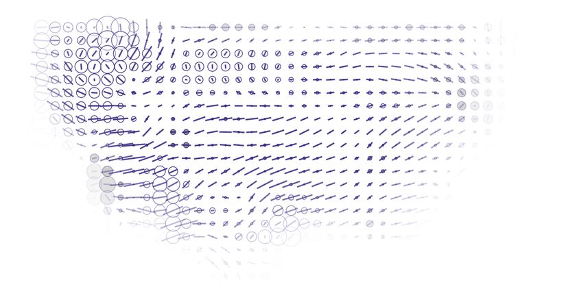
bioRxiv preprint first posted online Jul. 8, 2019; doi: http://dx.doi.org/10.1101/696252. The copyright holder for this preprint
(which was not peer-reviewed) is the author/funder, who has granted bioRxiv a license to display the preprint in perpetuity.
                             It is made available under a CC-BY-NC-ND 4.0 International license.

      9   midgut and elongating germ-band [Collinet et al., 2015, Lye et al., 2015, Dicko et al.,
     10   2017] of Drosophila embryo, between contracting wing hinge and expanding wing blade
     11   in Drosophila pupa [Etournay et al., 2015, Ray et al., 2015], or between invaginating neu-
     12   ral plate and covering epidermal ectoderm of Xenopus embryo [Brodland et al., 2010],
     13   provide examples of how mechanical force generated in one region can drive large scale
     14   deformation in adjacent regions. In these cases, the regions which behave di↵erently are
     15   easily distinguished by specific gene expressions.
     16        However, many tissues were found to be heterogeneous but without obvious boundary
     17   between such regions, leaving analysis limited to arbitrary regions drawn as a grid parallel
     18   to tissue axes (Fig. 1A), or regions expressing already known di↵erentiation maker
     19   genes. Measured tissue deformation rate showed a large heterogeneity (accompanied
     20   by a heterogeneity in cellular processes such as cell proliferation rate, cell division, cell
     21   rearrangement, change of cell shape), and smooth spatial variations across the tissue,
     22   in Drosophila notum in a developing pupa [Bosveld et al., 2012, Guirao et al., 2015]
     23   (Fig. 1B), Drosophila wing blade [Etournay et al., 2015], blastopore lip of Xenopus
     24   gastrula [Feroze et al., 2015], chick gastrula [Rozbicki et al., 2015, Firmino et al., 2016],
     25   mouse palatal epithelia [Economou et al., 2013], and mouse limb bud ectoderm [Lau
     26   et al., 2015]. Recent formalisms have enabled to measure and link quantitatively cellular
     27   processes with tissue deformation [Blanchard et al., 2009, Guirao et al., 2015, Etournay
     28   et al., 2015, Merkel et al., 2017]. However, cellular quantities also vary smoothly across
     29   the tissue. In addition, the causal relationship between cellular processes and tissue
     30   deformation is not always trivial, making it difficult to identify regions those actively
     31   drive morphogenesis and those passively deformed by adjacent regions.
     32        To study the spatial regulation of morphogenesis at tissue scale, we developed a new
     33   multi-technique pipeline to divide a tissue into sub-regions based on quantitative mea-
     34   surements of static or dynamic properties of cells or tissues. Our tissue segmentation
     35   pipeline consists of three steps: a first fast tissue segmentation attempted several times
     36   with random seeding, then merging these multiple tissue segmentations into a single
     37   one, then smoothing the resulting regions boundaries (Fig. 1C). We apply it to the

                                                                      3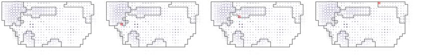
bioRxiv preprint first posted online Jul. 8, 2019; doi: http://dx.doi.org/10.1101/696252. The copyright holder for this preprint
(which was not peer-reviewed) is the author/funder, who has granted bioRxiv a license to display the preprint in perpetuity.
                             It is made available under a CC-BY-NC-ND 4.0 International license.

                            A                                              B

                            C
                              (1)                         (2)                         (3)
                                  Iterate tissue            Merge multiple              Smooth regions
                                 segmentations              segmentations                 boundaries

          Fig. 1: Morphogenesis of Drosophila pupa notum and overview of tissue segmentation
          pipeline. (A, B) Heterogeneity of tissue morphogenesis. Here a Drosophila notum at
          12 hr after pupa formation (APF), with arbitrary regions drawn from a grid (A), and
          at 32 hr APF, showing the heterogeneous deformation of previous regions using cell
          tracking (B). Cell patches are shown with blue and white check pattern. (C) Pipeline of
          the tissue segmentation. (1) Iteration of fast tissue segmentation with random seeding,
          using region growing algorithm. (2) Merging multiple tissue segmentations of step 1 into
          a single objective tissue segmentation, using label propagation algorithm on a consensus
          matrix. (3) Smoothing regions boundaries resulting of step 2, using cellular Potts model.

                                                                      4
bioRxiv preprint first posted online Jul. 8, 2019; doi: http://dx.doi.org/10.1101/696252. The copyright holder for this preprint
(which was not peer-reviewed) is the author/funder, who has granted bioRxiv a license to display the preprint in perpetuity.
It is made available under a CC-BY-NC-ND 4.0 International license.
38 morphogenesis of Drosophila pupa dorsal thorax. The first application is to the tissue
39 deformation rate integrated over the duration of a whole movie; the second application
40 is to the time evolution of this tissue deformation rate; and the third application is to
41 the time evolution of all cellular processes and their contribution to the local tissue de-
42 formation. Obtained sub-regions showed distinctive patterns of deformation and cellular
43 processes with higher homogeneity than those along tissue axes. Interestingly, the tissue
44 segmentations based on the local tissue deformation rate and on the cellular processes
45 included some similar regions, suggesting that the cellular processes were regulated sim-
46 ilarly inside the regions, therefore resulting in homogeneous tissue deformations inside
47 those regions.
48 3 Results I : Development of automatic tissue segmenta-
49 tion algorithm
50 3.1 Image segmentation by region growing algorithm
51 Finding distinctive and homogeneous regions inside the heterogeneous tissue amounts to
52 segmenting the geometrical space while keeping the points inside each of the regions as
53 similar as possible to each other in the property space. Here, we call property space any
54 morphogenesis quantification measured in the tissue, whereas geometrical space refers
55 to the two-dimensional space of cell patch positions inside the tissue.
56 Given a set of objects, collecting similar objects to divide them into groups is gener-
57 ally a task of cluster analysis. However, the cell patches distribute in the property space
58 and geometrical space. On the assumption that expression patterns of genes responsible
59 for morphogenesis make connected regions, and to study physical interactions between
60 the regions, we aimed at getting connected regions. The initial tissue segmentation first
61 defines a metric of similarity between cells, and then a tissue is divided into regions
62 containing similar cells. The image segmentation tool, called region growing [Adams
63 and Bischof, 1994, Ma et al., 2010] (Fig. 2A), was inspired by a study segmenting mouse
64 heart based on cell polarity [Le Garrec et al., 2013].
5bioRxiv preprint first posted online Jul. 8, 2019; doi: http://dx.doi.org/10.1101/696252. The copyright holder for this preprint
(which was not peer-reviewed) is the author/funder, who has granted bioRxiv a license to display the preprint in perpetuity.
It is made available under a CC-BY-NC-ND 4.0 International license.
65 To validate the algorithm, we first tested segmentation on a simple example, namely
66 the change in cell patch areas from 12 to 32 hr APF (Fig. 2B). The overall change in cell
67 patch areas defines the total tissue growth, while spatially heterogeneous changes in cell
68 patch areas result in local deformation, changes in tissue region proportions, and overall
69 tissue shape change. Technically speaking, the change in cell patch areas is a scalar
70 field, defined as the trace of the tissue deformation rate tensor. The region growing
71 succeeded in finding expanding regions in posterior, lateral posterior, and lateral parts
72 and a shrinking region in anterior part.
73 However, the results varied dependent on the initial seeds. In contrast to a segmenta-
74 tion in histology or of immuno-stained image, where a true segmentation is well defined,
75 the morphogenetic properties vary continuously with space, making it difficult to deter-
76 mine and validate the resultant segmentations. The silhouette, a measurement of region
77 homogeneity (the silhouette of an object would be 1 if it was similar to all objects in the
78 same cluster, and 1 if it was more similar to objects in other clusters), di↵ered from
79 one segmentation to the other (Fig. 2C). To assess the significancy of the homogeneity,
80 we compared it with the average silhouette of randomly made control segmentations.
81 Some of the region growing results had a low silhouette, even lower than that of half of
82 the control segmentations (Fig. 2C), which means they were lacking any signification.
83 A tissue segmentation method should return a unique result so that it could be com-
84 pared with gene expression patterns or fed forward to a study of mechanical interactions
85 between regions, but the region growing algorithm returned multiple results.
86 3.2 Defining a single tissue segmentation using label propagation on a
87 consensus matrix
88 To obtain a single tissue segmentation, we turned to consensus clusterings. In fact, since
89 resultant segmentations of the region growing were dependent on randomly given initial
90 values, we ran multiple trials and merged multiple segmentation results into a single
91 one. Given multiple partitions, the consensus clustering returns the partition which is
92 the most similar to all of the initial partitions. We tried several consensus clustering
6bioRxiv preprint first posted online Jul. 8, 2019; doi: http://dx.doi.org/10.1101/696252. The copyright holder for this preprint
(which was not peer-reviewed) is the author/funder, who has granted bioRxiv a license to display the preprint in perpetuity.
It is made available under a CC-BY-NC-ND 4.0 International license.
A
…
-0.016 0.016
B expansion rate
C
Frequency
Silhouette
—ctrl, —rg
Fig. 2: Tissue segmentation by region growing algorithm. Tissue local expan-
sion/contraction rate is represented by size of white/gray circles. (A) Process of re-
gion growing algorithm. Points of given number (6 in the shown example) are chosen
randomly as initial seeds of regions, and the regions are expanded by collecting points
similar to the seeds from their neighbors. Once the field is segmented, the seeds are
updated to region centroids in the geometrical space and means in the property space,
and the expansion of the regions are performed again from the new seeds. The seeds are …
shown with colored square, where the color represents an expansion rate of the regions.
The regions are colored lighter for visibility. This update of the seeds and the regions are
iterated until it reaches a convergence. (B) Four example results of region growing. (C)
Histogram of silhouette value: blue for control segmentations, orange for region growing.
Dotted vertical orange lines show silhouette values of the four examples shown in B.
AOA_big_20h_olap_0/3/trG_1.6.rg.{2,
4, 7, 8}.tif
93 algorithms, and found the label propagation on a consensus matrix [Lancichinetti and
94 Fortunato, 2012, Raghavan et al., 2007] returning the best segmentation, while others
7bioRxiv preprint first posted online Jul. 8, 2019; doi: http://dx.doi.org/10.1101/696252. The copyright holder for this preprint
(which was not peer-reviewed) is the author/funder, who has granted bioRxiv a license to display the preprint in perpetuity.
It is made available under a CC-BY-NC-ND 4.0 International license.
95 returned many disconnected regions or single point regions (data not shown).
96 The label propagation on a consensus matrix converted multiple tissue segmentations
97 into a weighted graph where weight of an edge represented a frequency of segmentations
98 in which incident vertices (points) belonged to the same region (Fig. 3A). Then labels on
99 the vertices were propagated according to the weight so that the same label was assigned
100 to points which were frequently included in the same region among the given multiple
101 region growing segmentations.
102 The label propagation returned results similar to the region growing segmentations
103 (Fig. 2B, 3B). Also, the label propagation results were more similar to each other than
104 results of region growing, assessed with adjusted Rand indices (ARI), a measurement
105 of similarity between two partitions (ARI of identical partitions would be 1). ARI were
106 0.50 ± 0.21 among the results of the region growing and 0.97 ± 0.02 among the results of
107 the label propagation. They showed similar average silhouette values, similar to median
108 of those of region growing results, but smaller than the highest value of those of region
109 growing (Fig. 3C). The average silhouette of the label propagation result was higher
110 than those of 99.95% of the randomly made control segmentations.
111 However, the label propagation algorithm does not assure the connectedness of re-
112 gions (Fig. 3C lower panels). Also, contour of regions may be complex (data not shown).
113 3.3 Smoothing of tissue segmentation results by cellular Potts model
114 The consensus region boundaries were then smoothed by cellular Potts model, which
115 balances the decrease in the length of region boundaries with the preservation of region
116 area and homogeneity (Fig. 4A). It smoothed boundaries and removed disconnected
117 cell patches (Fig. 4B, C) while keeping the average silhouette higher than those of
118 random segmentations (Fig. 4D). Since the cellular Potts model simulation includes the
119 Metropolis update, i.e., choosing a pixel randomly and updating the pixel by probability
120 according to a change of the energy, resultant smoothed segmentations varied among
121 di↵erent trials even with the same parameters and initial segmentation (data not shown).
122 Now we have a pipeline of the region growing, the label propagation, and the cellular
8bioRxiv preprint first posted online Jul. 8, 2019; doi: http://dx.doi.org/10.1101/696252. The copyright holder for this preprint
(which was not peer-reviewed) is the author/funder, who has granted bioRxiv a license to display the preprint in perpetuity.
It is made available under a CC-BY-NC-ND 4.0 International license.
A
, , , , , ,
a a→e e
5 2 5 5 5
2 e b b e b→c
e
4 3 4 3 4 3 4 3
…
6 1 3 4 6 3 4 6 3 4 6 3 4
2 d c d c d c
B
C
Frequency
Silhouette
—ctrl, —rg, —lp
Fig. 3: Tissue segmentation by label propagation on a consensus matrix. (A) Process of
label propagation algorithm. Multiple clusterings (upper) are converted to a consensus
matrix, which gives weights to a complete graph on the objects being clustered (lower
left). Edges with weights less than a given threshold are removed. All objects are
initially assigned labels di↵erent to each other. And then, one by one in random order,
each label is updated to the most frequent one weighted by edges incident to the object
until it reaches a convergence. (B) Four example results of label propagation on the same
consensus matrix. (C) Histogram of silhouette value: blue for control segmentations,
orange for region growing, red for label propagation.
123 Potts model to divide a field of property (scalar, tensor, or any kind of value with metric)
124 into regions. The resultant regions are homogeneous, where points in each region are
9
AOA_big_20h_olap_0/3/trG_1.6.lp.
{1-4}.tifbioRxiv preprint first posted online Jul. 8, 2019; doi: http://dx.doi.org/10.1101/696252. The copyright holder for this preprint
(which was not peer-reviewed) is the author/funder, who has granted bioRxiv a license to display the preprint in perpetuity.
It is made available under a CC-BY-NC-ND 4.0 International license.
A
…
p < 0.005
B C D
Frequency
Silhouette
—ctrl, —rg, —lp, —smoothed
Fig. 4: Boundary smoothing by cellular Potts model. (A) Process of cellular Potts
model. A pixel is randomly chosen and changes its belonging region if it decreases
boundary length and/or increases homogeneity (marked by red). (B) Result of label
propagation with a disconnected region shown by gray color. (C) Result of boundary
smoothing by cellular Potts model. (D) Histogram of silhouette value: blue for control
segmentations, orange for region growing, red vertical line for label propagation, and
black vertical line for regions smoothed by cellular Potts model. Dotted blue line shows
threshold for the highest 0.5% of the control segmentations.
125 more similar to each other than to points in other regions.
126 4 Results II : Tissue segmentation based on tissue mor-
127 phogenesis
128 We now turn to property spaces better representing tissue morphogenesis. In Guirao
129 et al. [2015], tissue deformation rate (G) and underlying cellular processes, cell division
130 (D), cell rearrangement (R), cell shape change (S), and cell delamination (A) were
131 quantified into tensors. The tensors were obtained from change of the texture averaged
10bioRxiv preprint first posted online Jul. 8, 2019; doi: http://dx.doi.org/10.1101/696252. The copyright holder for this preprint
(which was not peer-reviewed) is the author/funder, who has granted bioRxiv a license to display the preprint in perpetuity.
It is made available under a CC-BY-NC-ND 4.0 International license.
132 over 20 hr from 12 hr APF to 32 hr APF or over 2 hr at each time point. By projecting
133 each tensor on the deformation rate, one can measure an amplitude of deformation rate
134 and an e↵ective contribution of cellular process, which represents how much the cellular
135 process contributes to the tissue deformation. They are scalar value and denoted by G//
136 for the deformation rate, D// for cell division, R// for cell rearrangement, S// for cell shape
137 change, and A// for cell delamination (see appendix). For the sake of clarity, we call the
138 tissue deformation rate and the cellular processes averaged over the whole 20 hr from 12
139 to 32 hr APF time-average tissue deformation rate and cellular processes.
140 The e↵ective contributions averaged over the whole tissue showed dynamic time
141 evolution (Fig. S1), with a large peak of cell division and cell shape change around 16
142 hr APF, second small wave of cell division around 22 hr APF, and gradual increase of
143 cell shape change and cell rearrangement. The e↵ective contributions also showed large
144 variance across the tissue at each time point.
145 4.1 Tissue segmentations based on time-evolution of deformation rate
146 and cellular processes e↵ective contributions
147 We first divided the tissue based on time-average and time-evolution of tissue defor-
148 mation rate. A distance between the tensor-valued functions was given by L2 -norm.
149 The notum was divided into anterior-middle-posterior and medial-lateral regions (Fig.
150 5A-D).
151 Next, we divided the tissue based on time-evolution of cellular processes. The ef-
152 fective contributions of the cellular processes were combined in a vector. For the time-
153 evolution of the cellular processes, a distance between the vector-valued function was
154 also given by L2 -norm. In contrast to segmentations based on the time-average and
155 time-evolution of deformation rate, the segmentations based on time-average and time-
156 evolution of the cellular processes e↵ective contribution vectors di↵ered from each other
157 (Fig. 5E-H). The resultant segmentation based on time-evolution included a posterior
158 region, a large middle region, a neck-notum boundary region, lateral posterior region, a
159 scutum-scutellum boundary region, and a lateral region (Fig. 5H).
11bioRxiv preprint first posted online Jul. 8, 2019; doi: http://dx.doi.org/10.1101/696252. The copyright holder for this preprint
(which was not peer-reviewed) is the author/funder, who has granted bioRxiv a license to display the preprint in perpetuity.
It is made available under a CC-BY-NC-ND 4.0 International license.
A B
C D
E F
G H
Fig. 5: Segmentations based on tissue deformation and underlying cellular processes.
Direction of elongation is represented by bars. For quantification and representation
of tissue deformation rate and cellular processes, see methodology and Guirao et al.
[2015]. (A-H) Segmentations based on time-average tissue deformation rate (A, B),
time-evolution of deformation rate (C, D), time-average cellular processes e↵ective con-
tributions (E. F), and time-evolution of cellular processes (G, H). First column shows
results of label propagation (A, C, E, G) and second column shows results of boundary
smoothing (B, D, F, H).
12bioRxiv preprint first posted online Jul. 8, 2019; doi: http://dx.doi.org/10.1101/696252. The copyright holder for this preprint
(which was not peer-reviewed) is the author/funder, who has granted bioRxiv a license to display the preprint in perpetuity.
It is made available under a CC-BY-NC-ND 4.0 International license.
160 4.2 Correspondence between segmentations based on cellular processes
161 and deformation rate
162 Both of the segmentations based on time-evolution of deformation rate and cellular
163 processes e↵ective contributions included the large anterior region, the middle boundary
164 region, the lateral posterior region, and the posterior region, although the anterior and
165 posterior regions were divided into medial and lateral subregions in the segmentation
166 based on the deformation rate. Figure 6A-D show overlap between segmentation based
167 on time-evolution of deformation rate (Fig. 5D) and the others (Fig. 5B, F, H) or a
168 conventional large grid parallel to tissue axes. Despite the overlap of the middle boundary
169 regions and the lateral posterior regions, ARI between the segmentations based on time-
170 evolution of deformation rate and cellular processes was not high (0.391) because of the
171 medial and lateral subregions in the anterior and posterior regions. The ARI value was
172 similar to those between others (Fig. 6E).
173 4.3 Homogeneity of the obtained regions
174 Next, we evaluated the homogeneity of the obtained regions. The time-evolution of
175 deformation rate was similar among cells inside regions of the segmentations based on
176 time-average and time-evolution of deformation rate except the middle-lateral region of
177 the former (Fig. 7A, B). On the other hand, the large grid segmentation showed large
178 heterogeneity in the posterior regions (Fig: 7C). The average silhouette value of the
179 segmentation based on the time-evolution of deformation rate was higher than those of
180 99.5% of the control segmentations (average silhouette for label propagation: 0.0568,
181 for smoothed regions: 0.0527, the maximum of the smallest 99.5% of controls average
182 silhouettes: 0.0425) (Fig. 7D). The average silhouette of the segmentation based on
183 time-averaged deformation rate was also higher than 95% of the control segmentations
184 (average silhouette for label propagation: 0.0336, for smoothed regions: 0.0107, the
185 maximum of the smallest 95% of controls average silhouettes: -0.0098). On the other
186 hand, that of the conventional grid segmentation was close to median of the control
187 segmentations (average silhouette: -0.0694).
13bioRxiv preprint first posted online Jul. 8, 2019; doi: http://dx.doi.org/10.1101/696252. The copyright holder for this preprint
(which was not peer-reviewed) is the author/funder, who has granted bioRxiv a license to display the preprint in perpetuity.
It is made available under a CC-BY-NC-ND 4.0 International license.
A B E
1
Adjusted Rand
index
0.5
C D 0
deformation rate
time-average
cellular processes
time-average
cellular processes
time-evolution
large grid
Fig. 6: Correspondence between segmentations based on cellular processes and deforma-
tion rate. (A-D) Overlays of segmentations, where segmentation based on time-evolution
of deformation rate is shown by cyan line, while segmentations based on time-average
deformation rate (A), time-average cellular processes (B), time-evolution of cellular pro-
cesses (C), and large grid (D) are shown by magenta line. (E) Adjusted Rand indices
of A-D. adjusted Rand index
12/plots.numbers
188 Sheet 1 inside the regions of
Also, the time-evolution of cellular processes was homogeneous
189 the segmentation based on time-evolution of cellular processes, but not in segmentation
190 based on time-average of cellular processes nor in the grid (Fig. 7E-G). The average
191 silhouette value of segmentation based on time-evolution was higher than 99.995% of
192 control segmentations (average silhouette for label propagation: 0.147, for smoothed
193 regions: 0.152, the maximum of the smallest 99.995% of controls average silhouettes:
194 0.124), while that of segmentation based on time-average was smaller than 5% of control
195 segmentations (average silhouette for label propagation: 0.012, for smoothed regions:
196 0.015, the maximum of the smallest 99.995% of controls average silhouettes: 0.024)
197 (Fig. 7H).
198 Our tissue segmentation is designed to divide a tissue into regions homogeneous in
199 a given property space, and the homogeneity of deformation rate in the segmentation
14bioRxiv preprint first posted online Jul. 8, 2019; doi: http://dx.doi.org/10.1101/696252. The copyright holder for this preprint
(which was not peer-reviewed) is the author/funder, who has granted bioRxiv a license to display the preprint in perpetuity.
It is made available under a CC-BY-NC-ND 4.0 International license.
200 based on the deformation rate demonstrated that the pipeline worked fine. Therefore,
201 it does not assure the homogeneity of regions in a property space di↵erent from one
202 based on which segmentation was performed. Figure S2 shows heat maps of silhouette
203 values measured in di↵erent property spaces. Homogeneity in the regions di↵ered among
204 the property spaces. However, the large anterior region in the segmentation based on
205 time-evolution of cellular processes was homogeneous in all property spaces. On the
206 other hand, the posterior region in the segmentation based on time-evolution of cellular
207 processes showed heterogeneity of deformation rate, while the two posterior regions in
208 the segmentation based on deformation rate showed homogeneity of cellular processes.
209 4.4 Cellular processes e↵ective contributions inside the regions
210 Figure 8 shows plots of cellular processes e↵ective contributions averaged in each region
211 of the segmentation based on time-evolution of deformation rate, where the medial and
212 lateral anterior regions were merged. The anterior region did not have the second peak
213 of cell divisions, while the first peak was small in the lateral posterior region. The two
214 posterior regions had di↵erent cell divisions and cell shape changes after the second peak
215 of cell division. The lateral regions showed cell shape changes between the two peaks of
216 cell division and increasing cell rearrangements.
217 Distances between the plots in Figure 8 (0.66 ± 0.16) were close to those between
218 plots in the segmentation based on time-evolution of cellular processes (0.67 ± 0.15) and
219 larger than those between plots in the large grid (0.44 ± 0.14) (Fig. S3). This result
220 demonstrates that cellular processes in the obtained segmentations were more distinctive
221 than those in the conventional grid.
222 5 Discussion
223 This study demonstrates that the pipeline of the region growing, the label propagation on
224 the consensus matrix, and the boundary smoothing by cellular Potts model could divide
225 a deforming heterogeneous tissue into homogeneous regions based on the morphogenetic
15bioRxiv preprint first posted online Jul. 8, 2019; doi: http://dx.doi.org/10.1101/696252. The copyright holder for this preprint
(which was not peer-reviewed) is the author/funder, who has granted bioRxiv a license to display the preprint in perpetuity.
It is made available under a CC-BY-NC-ND 4.0 International license.
p < 0.005
D
A B C
Frequency
Silhouette
H p < 0.0005
E F G
Frequency
-1 silhouette value 1
Silhouette
—ctrl, —rg, —lp, —smoothed, —t_average, —grid
Fig. 7: Homogeneity in the obtained regions. (A-C) Heat map of silhouette value mea-
sured with time-evolution of tissue deformation rate in segmentations based on time-
average deformation rate (A), time-evolution of deformation rate (B), and large grid
(C). (D) Histogram of silhouette value, : blue for control segmentations, orange for re-
gion growing. Red vertical lines show silhouette value of label propagation results. Black
vertical lines show silhouette value of regions smoothed by cellular Potts model. Dot-
ted blue lines show threshold for the highest 0.5% of the control segmentations. Gray
and cyan vertical line shows silhouette value of segmentation based on time-averaged
deformation rate and large grid. (E-G) Heat map of silhouette value measured with
time-evolution of cellular processes e↵ective contributions in segmentations based on
time-average cellular processes (E), time-evolution of cellular processes (F), and large
grid (G). (H) Histogram of silhouette value, : blue for control segmentations, orange
for region growing. Red vertical lines show silhouette value of label propagation re-
sults. Black vertical lines show silhouette value of regions smoothed by cellular Potts
model. Dotted blue lines show threshold for the highest 0.05% of the control segmen-
tations. Gray and cyan vertical line shows silhouette value of segmentation based on
time-averaged cellular processes and large grid.
16bioRxiv preprint first posted online Jul. 8, 2019; doi: http://dx.doi.org/10.1101/696252. The copyright holder for this preprint
(which was not peer-reviewed) is the author/funder, who has granted bioRxiv a license to display the preprint in perpetuity.
It is made available under a CC-BY-NC-ND 4.0 International license.
A B 0.15 0.12
1 2
2 3 0.1 0.08
Components
Components
0.05 0.04
1
0 0
-0.05 -0.04
-0.1 -0.08
4 5 -0.15 -0.12
13 16 19 22 25 28 31 13 16 19 22 25 28 31
Time (hr APF) Time (hr APF)
0.12 0.12 0.12
3 4 5
0.08 0.08 0.08
Components
Components
Components
0.04 0.04 0.04
0 0 0
-0.04 -0.04 -0.04
-0.08 -0.08 -0.08
-0.12 -0.12 -0.12
13 16 19 22 25 28 31 13 16 19 22 25 28 31 13 16 19 22 25 28 31
Time (hr APF) Time (hr APF) Time (hr APF)
— G// — D// — R// — S// — A//
Fig. 8: Cellular processes e↵ective contributions inside the regions. (A) Tissue segmen-
tation based on time-evolution of deformation rate, where two anterior subregions were
merged. (B) Plots of cellular processes e↵ective contributions averaged in each region
of 1-5 in A.
17bioRxiv preprint first posted online Jul. 8, 2019; doi: http://dx.doi.org/10.1101/696252. The copyright holder for this preprint
(which was not peer-reviewed) is the author/funder, who has granted bioRxiv a license to display the preprint in perpetuity.
It is made available under a CC-BY-NC-ND 4.0 International license.
226 properties. Using this segmentation, we found a large anterior region, a middle boundary
227 region, a lateral posterior region, and posterior regions that had distinctive deformation
228 rates and cellular processes time-evolutions.
229 The tissue segmentation based on morphogenesis di↵ers from conventional image seg-
230 mentations, cell segmentations, and other tissue segmentations those are an automation
231 of manual segmentation and can be corrected manually. First, the morphogenesis was
232 quantified as multiple tensor fields with time evolution, and thus it is hard to visualize
233 them in a 2D image for manual segmentation. Second, it is not easy to evaluate whether
234 given a region actually corresponds to genetical/mechanical regulation of morphogenesis.
235 Therefore we looked for a method which divides a tissue based on any kind of quantity
236 and returns regions with smooth boundaries. Region growing is a conventional and sim-
237 ple method of image segmentation, and requires a property space only to be metric. The
238 varying results of the region growing were given to the label propagation and cellular
239 Potts model to produce a single tissue segmentation, and the result was evaluated by
240 homogeneity of the regions and smoothness of the boundary.
241 The tissue segmentations based on time evolution of deformation rate and e↵ective
242 contributions of cellular processes returned similar results with large anterior regions,
243 posterior regions, lateral posterior regions, and middle boundary regions (Fig. 6). By
244 the deformation rate, the anterior and posterior regions were divided into medial and
245 lateral subregions. Since the vector of e↵ective contributions ignores the direction of
246 deformation, the two subregions could be interpreted as regions of similar underlying
247 cellular processes but deforming in di↵erent directions. On the other hand, the middle
248 boundary region and the lateral region given by the cellular processes, both overlapped
249 with the middle boundary region given by deformation rate, could be interpreted as
250 regions with di↵erent cellular processes but of similar deformations.
251 Silhouette analysis showed that the segmentations based on time-evolution of de-
252 formation rate and cellular processes included regions homogeneous in various property
253 spaces, whereas the conventional grid segmentation included heterogeneous regions. Es-
254 pecially, the large anterior region showed high homogeneity of deformation rate and the
18bioRxiv preprint first posted online Jul. 8, 2019; doi: http://dx.doi.org/10.1101/696252. The copyright holder for this preprint
(which was not peer-reviewed) is the author/funder, who has granted bioRxiv a license to display the preprint in perpetuity.
It is made available under a CC-BY-NC-ND 4.0 International license.
255 two posterior subregions showed high homogeneity of cellular processes.
256 In conclusion, we built a method to divide a tissue based on any kind of property
257 space. This allows an application to a study of spatial regulation of various processes,
258 where the property space should be chosen for the process of interest. For example,
259 to study a spatial regulation of cell division orientation, the property space may be
260 prepared from, instead of the local deformation rate and cellular processes, the tensor
261 field of cell division and known regulating factors such as cell shape, localization of planar
262 cell polarity proteins, and tension on cell-cell interface, and then resultant regions can
263 be compared with genes expression patterns.
264 6 Methods
265 6.1 Quantification tools
266 Morphogenesis data result from the quantification of local tissue deformation rate and
267 underlying cellular processes as described in [Guirao et al., 2015]. The similarity be-
268 tween two tensors is quantified by the standard Euclidian metric. The homogeneity of
269 a quantity within a given region, i.e. the similarity between measurements of this quan-
270 tity within a region, is measured by silhouette, a standard tool of cluster analysis. For a
271 measurement of similarity between tissue segmentations, we use the Rand index, which
272 indicates how well two data clusterings agree.
273 6.1.1 Quantification of tissue deformation and cellular processes
274 Quantification of local tissue deformation and underlying cellular processes was per-
275 formed in [Guirao et al., 2015]. Briefly, Drosophila nota expressing GFP-tagged E-
276 cadherin were imaged. The notum movies were split in a grid (with patches about 20
277 µm width) at the first frame (Fig. 1C), 12 hr after pupa formation (APF). The local
278 deformation rate and the cellular processes were measured in each cell patch through
279 the development, as follows.
280 Epithelial cells contours were detected automatically using watershed algorithm, the
19bioRxiv preprint first posted online Jul. 8, 2019; doi: http://dx.doi.org/10.1101/696252. The copyright holder for this preprint
(which was not peer-reviewed) is the author/funder, who has granted bioRxiv a license to display the preprint in perpetuity.
It is made available under a CC-BY-NC-ND 4.0 International license.
281 cells were tracked, adjacencies between cells were listed, and relative positions of centers
282 of adjacent cells were recorded. The tissue deformation rate, denoted by the symmetric
283 tensor G, was obtained from change of relative positions between neighbor cells over
284 20 hr from 12 hr APF to 32 hr APF, or over 2 hr at each time point when recording
285 the time evolution. The tissue deformation rate G was then decomposed into cell shape
286 change S and deformation accompanied by change of cell adjacency, which was further
287 divided into cell division D, cell rearrangement R, and cell delamination A, which are
288 symmetric tensors too.
289 In a collection of cells where the total deformation is driven completely by the four
290 fundamental cellular processes, the tensors are in a balance equation,
G = D + R + S + A. (1)
291 The scalar product of two tensors Q and Q0 in dimension d is defined as:
1
Q.Q0 = Tr(QQ0T ), (2)
d
292 and the unitary tensor uG that is aligned with G is given by
G
uG = . (3)
(G.G)1/2
Since the scalar product (Eqn. 2) is a linear transformation, multiplying uG by a tensor,
the operation .uG : Q ! Q//, retains the balance between the tissue deformation rate
and the cellular processes in Equation 1 while converting them to magnitudes:
G// =G.uG
=(D + R + S + A).uG
=D.uG + R.uG + S.uG + A.uG
=D// + R// + S// + A//. (4)
293 The scalar G// represents the local magnitude of tissue morphogenesis, and D//, R//,
294 S//, and A// represent the e↵ective contributions of the cellular processes to the tissue
295 morphogenesis. When a cellular process produces an anisotropic deformation in the
20bioRxiv preprint first posted online Jul. 8, 2019; doi: http://dx.doi.org/10.1101/696252. The copyright holder for this preprint
(which was not peer-reviewed) is the author/funder, who has granted bioRxiv a license to display the preprint in perpetuity.
It is made available under a CC-BY-NC-ND 4.0 International license.
296 same direction with that of tissue, e.g. cells divided in the same direction with tissue
297 elongation, the scalar product between the them returns a positive value, while it returns
298 negative value when a cellular process counteractes tissue deformation.
299 6.1.2 Metric
300 Similarity of morphogenesis between the cell patches was defined as follows.
301 For expansion/contraction of area (isotropic deformation), similarity was given by
302 di↵erence in expansion/contraction rates.
303 Similarity of anisotropic deformation was given by a distance between two tensors Q
304 and Q’,
(✓ ◆2 )1/2
Qxx Qyy Q’xx Q’yy
d(Q, Q’) = + (Qxy Q’xy )2 . (5)
2 2
305 For tensors with time-evolution Q(t) and Q’(t), distance was given by a sum of
306 distance at each time point,
Z
|Q Q’| = d(Q(t), Q’(t))dt, (6)
307 as an analogy to L1 -norm between functions.
308 For the composition of cellular processes, the tensors of cellular processes were con-
309 verted to e↵ective contributions and combined into a vector (G//, D//, R//, S//, A//). A
310 distance between two vectors was given by L2 -norm, and a distance between vector-
311 valued functions v(t) and v 0 (t) was given by an integral of the L2 -norm between v(t) and
312 v 0 (t),
Z
0
|v v|= ||v(t) v 0 (t)||dt. (7)
313 6.1.3 Silhouette and bootstrap
314 Silhouette quantifies clustering results, indicating how well an object resembles other
315 objects inside its own cluster [Rousseeuw, 1987]. For object p, the silhouette value of p
316 is defined by
b(p) a(p)
s(p) = , (8)
max{a(p), b(p)}
21bioRxiv preprint first posted online Jul. 8, 2019; doi: http://dx.doi.org/10.1101/696252. The copyright holder for this preprint
(which was not peer-reviewed) is the author/funder, who has granted bioRxiv a license to display the preprint in perpetuity.
It is made available under a CC-BY-NC-ND 4.0 International license.
317 where a(p) is an average distance from p to other objects in the same cluster, and b(p)
318 is the smallest average distance from p to all objects in any other clusters. By this
319 definition, 1 s(p) 1, where s(p) large and close to 1 indicates that p is similar
320 to other objects in the same cluster, while negative s(p) indicates that there is another
321 cluster whose objects are more similar to p than objects in the cluster containing p.
322 We took the average silhouette value over all points (cell patches) as a measurement
323 of homogeneity of a given segmentation. For significance test, tissue was segmented ran-
324 domly 20,000 times into a given number, and we got thresholds above which the highest
325 5%, 0.5%, or 0.005% of the average silhouettes were found. The average silhouette of
326 given regions were compared to those of the control segmentations with the same number
327 of regions.
328 6.1.4 Adjusted Rand index
329 For a measurement of similarity between tissue segmentations, we use the Rand index,
330 which indicates how well two data clusterings agree ; its value is 1 if the clusterings
331 entirely disagree and 1 if they entirely agree. Its corrected-for-chance version is a more
332 meaningful quantity, called the adjusted Rand index (ARI): it is the Rand index minus
333 its value expected for the random case, and its value can be negative.
334 We compute the adjusted Rand index with the permutation model [Hubert and
335 Arabie, 1985]. Given two clusterings A = {A1 , . . . , Ak } and B = {B1 , . . . , Bm } of N
336 elements, the contingency table ⌧ = (nij )k⇥m is made where nij = |Ai \ Bj |. The Rand
337 index between A and B, RI(A, B) is given by the function
0 1 0 1 0 1 0 1
P nij P ai P bj N
2 ij @ A i
@ A
j
@ A+@ A
2 2 2 2
RI(A, B) = 0 1 , (9)
N
@ A
2
P P
338 where ai = j nij and bj = i nij , and an expected Rand index E[RI(A, B)] is given
22bioRxiv preprint first posted online Jul. 8, 2019; doi: http://dx.doi.org/10.1101/696252. The copyright holder for this preprint
(which was not peer-reviewed) is the author/funder, who has granted bioRxiv a license to display the preprint in perpetuity.
It is made available under a CC-BY-NC-ND 4.0 International license.
339 by the function
0 1 0 1 0 0 11 0 0 11
P a P bj P ai C B P bj C
@ iA @ A B
B @ AC B @ AC
i j i j
2 2 B 2 C B 2 C
B CB C
E[RI(A, B)] = 0 1 0 1 + B1 0 1 C B1 0 1 C. (10)
B CB C
N N B N CB N C
@ A @ A @ @ A A@ @ A A
2 2 2 2
340 The adjusted Rand index ARI(A, B) is given by the function
RI(A, B) E[RI(A, B)]
ARI(A, B) = . (11)
1 E[RI(A, B)]
341 6.2 Tissue segmentation pipeline
342 The pipeline was implemented by custom Matlab scripts, in three steps (Fig. 1C).
343 6.2.1 Region growing tissue segmentation
344 The initial tissue segmentation first defines a metric of similarity between cells, and then
345 a tissue is divided into regions containing similar cells. This approach was inspired by a
346 study segmenting mouse heart based on cell polarity [Le Garrec et al., 2013]. Testing k-
347 means clustering in the property space returned disconnected regions in the geometrical
348 space (data not shown). On the assumption that expression patterns of genes responsible
349 for morphogenesis make connected regions, and to study physical interactions between
350 the regions, we aimed at getting connected regions.
351 The algorithm Region growing [Adams and Bischof, 1994, Ma et al., 2010] is an
352 image segmentation method using a process similar to k-means clustering, starting from
353 randomly given seeds (corresponding to “means” in k-means clustering), segmenting an
354 image with the seeds followed by update of the seeds within the regions, and iterating this
355 process until convergence (Fig. 2A). The tissue segmentation is done by growing regions
356 from the seeds collecting pixels adjacent to the growing regions, and so the resultant
357 regions are connected.
358 Initial seeds were randomly chosen from data, and regions were expanded by adding
359 a pixel (cell patch) adjacent to a region and the most similar to the seed of the region
23bioRxiv preprint first posted online Jul. 8, 2019; doi: http://dx.doi.org/10.1101/696252. The copyright holder for this preprint
(which was not peer-reviewed) is the author/funder, who has granted bioRxiv a license to display the preprint in perpetuity.
It is made available under a CC-BY-NC-ND 4.0 International license.
360 in the property space one by one until all pixels were assigned to one of the regions.
361 The seeds were updated to pixels the closest to centroids of the regions, averages of
362 the regions in the property space were given as property of the seeds, and then regions
363 were expanded again from the seeds. These region expansions and seeds updates were
364 iterated until convergence was reached.
365 6.2.2 Label propagation on a consensus matrix
366 To merge multiple segmentation results into a single one independent on the metric, we
367 use label propagation algorithm on a consensus matrix, which takes multiple partitions
368 and returns a consensus partition which is the most similar to all partitions [Lancichinetti
369 and Fortunato, 2012, Raghavan et al., 2007].
370 For a division of n points, independent 50 trials of region growing were converted
371 to a consensus matrix, whose entry at i-th row and j-th column indicates a frequency
372 of partitions in which i-th point and j-th point were in the same cluster. The entries
373 lower than a given threshold were set to 0. The label propagation started by assigning to
374 each point a di↵erent label. Then the label of randomly chosen i-th point was updated
375 to one that was the most weighted by the consensus matrix, where ij element gave the
376 weight to a label of j-th point. The label update was iterated until convergence. The
377 threshold for the consensus matrix was scanned between 20-80% so that a resultant
378 partition contained the same number of regions as the initial partitions.
379 6.2.3 Cellular Potts model
380 To smooth the consensus region boundaries while preserving region area and homogene-
381 ity, we use the cellular Potts model, in which a cellular structure is numerically simulated
382 in a square lattice, where each cell is a set of pixels ; the pattern is updated to decrease the
383 energy, with some fluctuation allowance [Graner and Glazier, 1992]. In the simplest and
384 common two-dimensional form, the energy H arises from total perimeter length P (with
385 line energy J) and constraint on each region area A (with compressibility ); decreasing
386 it results in smoother region with preserved area A0 , removing small protrusions and
24bioRxiv preprint first posted online Jul. 8, 2019; doi: http://dx.doi.org/10.1101/696252. The copyright holder for this preprint
(which was not peer-reviewed) is the author/funder, who has granted bioRxiv a license to display the preprint in perpetuity.
It is made available under a CC-BY-NC-ND 4.0 International license.
387 disconnected regions. In this study, we also included the silhouette s to account for the
P ⇥ ⇤
388 region homogeneity, with a weight coefficient h: H = regions JP + (A A0 )2 hs .
389 The coefficients J, , and h were adjusted manually on a case by case basis.
390 When updating the label for a randomly selected pixel a, a target label was ran-
391 domly selected from neighbors of a, and then change of the Hamiltonian was calculated
392 and updated label of a to the target label with probability min(1, e H/T ), where H
393 denotes change of H by the change of label of a, and T is the fluctuation allowance. Sim-
394 ulations were iterated 100 times, then the result was visually inspected to check whether
395 boundaries were enough smooth, and if needed were iterated up to 400 times.
396 7 Acknowledgement
397 The authors thank Floris Bosveld for imaging, Stéphane U. Rigaud for cell segmentation
398 and tracking, Yohanns Bellaı̈che for directing and advises, and all team members for
399 insightful discussions.
400 8 Competing interests
401 The authors declare no competing nor financial interests.
402 9 Author contributions
403 Quantification of morphogenesis: B.G.; Methodology: S.Y., F.G.; Definition of metric:
404 S.Y., F.G.; Programming and implementation: S.Y.; Writing and editing: S.Y., F.G.;
405 Supervision: F.G.
406 10 Funding
407 This research was supported by grants from Uehara Memorial Foundation (201630059),
408 Japan Society for the Promotion of Science (201860572).
25bioRxiv preprint first posted online Jul. 8, 2019; doi: http://dx.doi.org/10.1101/696252. The copyright holder for this preprint
(which was not peer-reviewed) is the author/funder, who has granted bioRxiv a license to display the preprint in perpetuity.
It is made available under a CC-BY-NC-ND 4.0 International license.
409 References
410 R. Adams and L. Bischof. Seeded region growing. IEEE Trans Pattern Anal Mach Intell,
411 16:641–647, Jun 1994.
412 G. B. Blanchard, A. J. Kabla, N. L. Schultz, L. C. Butler, B. Sanson, N. Gorfinkiel,
413 L. Mahadevan, and R. J. Adams. Tissue tectonics: morphogenetic strain rates, cell
414 shape change and intercalation. Nat Methods, 6:458–464, 2009.
415 F. Bosveld, I. Bonnet, B. Guirao, S. Tlili, Z. Wang, A. Petitalot, R. Marchand, P.-L.
416 Bardet, P. Marcq, F. Graner, and Y. Bellaı̈che. Mechanical control of morphogenesis
417 by fat/dachsous/four-jointed planar cell polarity pathway. Science, 336:724–727, 2012.
418 G. W. Brodland, X. Chen, P. Lee, and M. Marsden. From genes to neural tube defects
419 (ntds): insights from multiscale computational modeling. HFSP J, 4:142–152, 2010.
420 C. Collinet, M. Rauzi, P.-F. Lenne, and T. Lecuit. Local and tissue-scale forces drive
421 oriented junction growth during tissue extension. Nat Cell Biol, 17:1247–1258, 2015.
422 M. Dicko, P. Saramito, G. B. Blanchard, C. M. Lye, B. Sanson, and J. Etienne. Geometry
423 can provide long-range mechanical guidance for embryogenesis. PLoS Comput. Biol.,
424 13(3):e1005443, Mar 2017.
425 A. D. Economou, L. J. Brock, M. T. Cobourne, and J. B. Green. Whole population
426 cell analysis of a landmark-rich mammalian epithelium reveals multiple elongation
427 mechanisms. Development, 140(23):4740–4750, Dec 2013.
428 R. Etournay, M. Popović, M. Merkel, A. Nandi, C. Blasse, B. Aigouy, H. Brandl, G. My-
429 ers, G. Salbreux, F. Julicher, and S. Eaton. Interplay of cell dynamics and epithelial
430 tension during morphogenesis of the Drosophila pupal wing. Elife, 4:e07090, Jun 2015.
431 R. Feroze, J. H. Shawky, M. von Dassow, and L. A. Davidson. Mechanics of blastopore
432 closure during amphibian gastrulation. Dev. Biol., 398(1):57–67, Feb 2015.
26bioRxiv preprint first posted online Jul. 8, 2019; doi: http://dx.doi.org/10.1101/696252. The copyright holder for this preprint
(which was not peer-reviewed) is the author/funder, who has granted bioRxiv a license to display the preprint in perpetuity.
It is made available under a CC-BY-NC-ND 4.0 International license.
433 J. Firmino, D. Rocancourt, M. Saadaoui, C. Moreau, and J. Gros. Cell Division Drives
434 Epithelial Cell Rearrangements during Gastrulation in Chick. Dev. Cell, 36(3):249–
435 261, Feb 2016.
436 F. Graner and J. A. Glazier. Simulation of biological cell sorting using a two-dimensional
437 extended Potts model. Phys. Rev. Lett., 69(13):2013–2016, Sep 1992.
438 B. Guirao, S. U. Rigaud, F. Bosveld, A. Bailles, J. Lopez-Gay, S. Ishihara, K. Sugimura,
439 F. Graner, and Y. Bellaı̈che. Unified quantitative characterization of epithelial tissue
440 development. Elife, 4, Dec 2015.
441 L. Hubert and P. Arabie. Comparing partitions. Journal of Classification, 2:193–218,
442 1985.
443 A. Lancichinetti and S. Fortunato. Consensus clustering in complex networks. Sci Rep,
444 2:336, 2012.
445 K. Lau, H. Tao, H. Liu, J. Wen, K. Sturgeon, N. Sorfazlian, S. Lazic, J. T. A. Burrows,
446 M. D. Wong, D. Li, S. Deimling, B. Ciruna, I. Scott, C. Simmons, R. M. Henkelman,
447 T. Williams, A.-K. Hadjantonakis, R. Fernandez-Gonzalez, Y. Sun, and S. Hopyan.
448 Anisotropic stress orients remodelling of mammalian limb bud ectoderm. Nat Cell
449 Biol, 17:569–579, 2015.
450 J. F. Le Garrec, C. V. Ragni, S. Pop, A. Dufour, J. C. Olivo-Marin, M. E. Bucking-
451 ham, and S. M. Meilhac. Quantitative analysis of polarity in 3D reveals local cell
452 coordination in the embryonic mouse heart. Development, 140(2):395–404, Jan 2013.
453 C. M. Lye, G. B. Blanchard, H. W. Naylor, L. Muresan, J. Huisken, R. J. Adams, and
454 B. Sanson. Mechanical Coupling between Endoderm Invagination and Axis Extension
455 in Drosophila. PLoS Biol., 13(11):e1002292, 2015.
456 Z. Ma, J. M. Tavares, R. N. Jorge, and T. Mascarenhas. A review of algorithms for
457 medical image segmentation and their applications to the female pelvic cavity. Comput
458 Methods Biomech Biomed Engin, 13(2):235–246, 2010.
27bioRxiv preprint first posted online Jul. 8, 2019; doi: http://dx.doi.org/10.1101/696252. The copyright holder for this preprint
(which was not peer-reviewed) is the author/funder, who has granted bioRxiv a license to display the preprint in perpetuity.
It is made available under a CC-BY-NC-ND 4.0 International license.
459 M. Merkel, R. Etournay, M. Popović, G. Salbreux, S. Eaton, and F. Julicher. Triangles
460 bridge the scales: Quantifying cellular contributions to tissue deformation. Phys Rev
461 E, 95(3-1):032401, Mar 2017.
462 G. Perez-Mockus, K. Mazouni, V. Roca, G. Corradi, V. Conte, and F. Schweisguth. Spa-
463 tial regulation of contractility by Neuralized and Bearded during furrow invagination
464 in Drosophila. Nat Commun, 8(1):1594, Nov 2017.
465 U. N. Raghavan, R. Albert, and S. Kumara. Near linear time algorithm to detect
466 community structures in large-scale networks. Phys Rev E Stat Nonlin Soft Matter
467 Phys, 76(3 Pt 2):036106, Sep 2007.
468 M. Rauzi, U. Krzic, T. E. Saunders, M. Krajnc, P. Ziherl, L. Hufnagel, and M. Lep-
469 tin. Embryo-scale tissue mechanics during Drosophila gastrulation movements. Nat
470 Commun, 6:8677, 2015.
471 R. P. Ray, A. Matamoro-Vidal, P. S. Ribeiro, N. Tapon, D. Houle, I. Salazar-Ciudad,
472 and B. J. Thompson. Patterned Anchorage to the Apical Extracellular Matrix Defines
473 Tissue Shape in the Developing Appendages of Drosophila. Dev. Cell, 34(3):310–322,
474 Aug 2015.
475 P. Rousseeuw. Silhouettes: a graphical aid to the interpretation and validation of cluster
476 analysis. Computational and Applied Mathematics, 20:53–65, 1987.
477 E. Rozbicki, M. Chuai, A. I. Karjalainen, F. Song, H. M. Sang, R. Martin, H.-J. Knölker,
478 M. P. MacDonald, and C. J. Weijer. Myosin-ii-mediated cell shape changes and cell
479 intercalation contribute to primitive streak formation. Nat Cell Biol, 17:397–408, 2015.
28You can also read