Quantitative Comparison between the Smartphone Based Experiments for the Gravity Acceleration Measurement at Home
←
→
Page content transcription
If your browser does not render page correctly, please read the page content below
education
                sciences
Article
Quantitative Comparison between the Smartphone Based
Experiments for the Gravity Acceleration Measurement
at Home
Marco Anni

                                          Dipartimento di Matematica e Fisica “Ennio De Giorgi”, Università del Salento, 73100 Lecce, Italy;
                                          marco.anni@unisalento.it

                                          Abstract: Smartphones are currently proposed as potential portable laboratories to perform a wide
                                          variety of physical experiments for teaching purpose. However, the frequent lack of clarity about
                                          the ease of replication of the experiments and on their accuracy often limits their effective use.
                                          In this work we deeply compare several smartphone-based experiments to determine the gravity
                                          acceleration g by only using cheap materials easily available at home. The experiment and the data
                                          analysis complexity are progressively increased, starting from fast and easy to replicate methods.
                                          The advantages and possible limits of all the methods are deeply discussed in order to allow an
                                          evaluation of the most suitable method for any particular teaching scenario.

                                          Keywords: physics at home; smartphone; classical mechanics; physics teaching


                                   1. Introduction
Citation: Anni, M. Quantitative                The possibility of performing experiments is a fundamental aspect of physics learning.
Comparison between the Smartphone         Unfortunately, the necessity of a suitably equipped didactic laboratory often strongly limits,
Based Experiments for the Gravity         or even prevents, the inclusion of practical activities not only at high school level, but
Acceleration Measurement at Home.         often also in university courses with a too high number of students. For this reason, the
Educ. Sci. 2021, 11, 493. https://
                                          development of experimental techniques able to avoid the use of a standard laboratory is
doi.org/10.3390/educsci11090493
                                          extremely important.
                                               In this frame, the recent demonstration of the possibility to exploit the camera or the
Academic Editors: Diego Vergara and
                                          internal sensors of common smartphones for a wide variety of physical experiments can
Ismo T. Koponen
                                          potentially be a real revolution [1–3]. For example, it has been shown that a smartphone
                                          camera can be used as light sensor in homemade spectrometers [4], or as indirect posi-
Received: 15 July 2021
Accepted: 25 August 2021
                                          tion sensors in mechanics experiments based on video analysis[5]. Another extremely
Published: 1 September 2021
                                          interesting possibility is the use of the data coming from the internal sensors, like the
                                          accelerometer, the light meter, the microphone, the magnetometer and so on, to perform
Publisher’s Note: MDPI stays neutral
                                          experiments of mechanics [5,6], magnetism [7], acoustic [8,9] and optics [10,11]. Access to
with regard to jurisdictional claims in
                                          the sensors data is nowadays made straightforward by the development of specific free
published maps and institutional affil-   apps, like Physics Toolbox Sensor Suite or Phyphox [12], really allowing anybody to easily
iations.                                  transform their smartphone into a potentially extremely versatile portable laboratory. This
                                          possibility is amazing, as it potentially paves the way for the execution of quantitative
                                          physics experiments in a classroom in which each student has his/her own instrument, or
                                          even to experiments performed individually at home.
Copyright: © 2021 by the authors.
                                               For these reasons, smartphone-based physics teaching is currently receiving huge
Licensee MDPI, Basel, Switzerland.
                                          attention, also documented by editorials in journals from American Physical Society [13]
This article is an open access article
                                          and Springer Nature [14], and proposals of smartphone base experiments can be found not
distributed under the terms and           only in professional journals, but also on web-pages and video sharing platforms.
conditions of the Creative Commons             Among the different proofs of concepts of smartphone-based physical experiments,
Attribution (CC BY) license (https://     the possibility to measure gravity acceleration g is one of the most important for high
creativecommons.org/licenses/by/          school and university students, as the vertical free fall motion is typically proposed as an
4.0/).                                    example of uniformly accelerated linear motion.

Educ. Sci. 2021, 11, 493. https://doi.org/10.3390/educsci11090493                                           https://www.mdpi.com/journal/education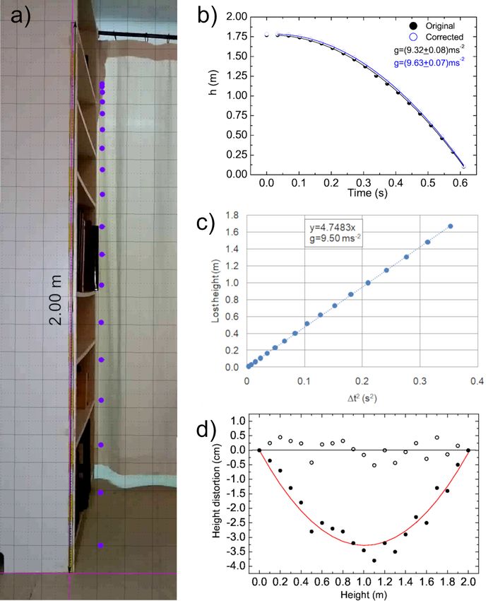
Educ. Sci. 2021, 11, 493                                                                                               2 of 20

                                When a body is left to fall with initial vertical velocity, assuming negligible drag
                           viscous air resistance and a constant gravitational attraction force, it is well known that the
                           motion temporal law is given by:

                                                                    1                            1
                                          y(t) = h + v0y (t − t0 ) − g(t − t0 )2 = h + v0y (∆t) − g(∆t)2                  (1)
                                                                    2                            2
                           where y(t) is the body height at time t measured along a vertical axis, oriented upwards,
                           and with origin on the ground level, h is the initial height, v0y is the vertical component of
                           the initial velocity, g is the modulus of the gravity acceleration and t0 is the initial instant.
                           We remember that t0 is not necessarily the time instant in which the motion starts, but can
                           also simply be the instant in which the height is h and the velocity vertical component is
                           v0y . Assuming that t0 is the instant in which the motion starts and that the body starts to
                           fall from rest, it is immediate to show that Equation (1) reduces to:

                                                                 1                 1
                                                       y(t) = h − g(t − t0 )2 = h − g(∆t)2                                (2)
                                                                 2                 2
                                Starting from this equation, it is straightforward to demonstrate that the time needed to
                           reach the ground (∆t f = t f − t0 ) is related to g value and the initial height h by the equation:

                                                                                2
                                                                       ∆t2f =     h                                       (3)
                                                                                g

                           and, just reversing the previous Equation, the g value can be obtained as:

                                                                            2h
                                                                       g=                                                 (4)
                                                                            ∆t2f

                                 Unfortunately, a direct experimental investigation of the free fall motion is absolutely
                           not trivial because the velocity of a falling object is too high to allow the manual mea-
                           surement of the position as a function time, preventing the determination of the motion
                           temporal law and the experimental proof of Equation (2).
                                 In a similar way, Equation (4) potentially allows to determine g by simply measuring
                           the time needed to reach the ground from a known starting height of any object in free
                           fall, but this experiment is complicated by the small values of ∆t f when the starting
                           height is within the range simply accessible at home (∆t f ≈ 0.45 s if h = 1.0 m, assuming
                           g = 9.8 ms−2 ). This prevents to manually measure the falling time, as it is of the same order
                           of magnitude of the error related to the reaction time.
                                 For these reasons the measurement of g from the free fall analysis typically requires
                           experimental set-up too complex to be replicated by a student [15–20], limiting the deter-
                           mination of the gravity acceleration with easy techniques to indirect measurements based,
                           for example, on the periodicity of the simple pendulum oscillation or of bodies attached to
                           elastic springs.
                                 These problems were well known already at the beginning of modern science and,
                           for example, led Galileo Galilei to use inclined planes to slow down the motion of rolling
                           spheres, or to investigate (or guess as it is not sure that the experiment was really done) the
                           dependence of the falling time on the mass for objects falling by high buildings, like the
                           Pisa Tower.
                                 A potential breakthrough in the g measurements from the free fall analysis is the
                           demonstration, in the last few years, of several smartphone-based techniques to perform
                           the measurement.
                                 The most widely used method is based on the determination of the falling time from a
                           known initial height, measuring the falling time by the internal accelerometer [6], from the
                           video of the motion filmed by the smartphone camera [21] or with the Phyphox acoustic
                           stopwatch [22].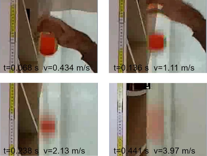
Educ. Sci. 2021, 11, 493                                                                                           3 of 20

                                Even more interesting is the possibility to determine the motion temporal law from the
                           video of the motion combined with video analysis [23] with free Software such as Tracker [24].
                                However, a general problem of all these proof of concept demonstrations of smartphone-
                           based physical measurements is the frequent lack of clarity on their real ease and on the
                           possible accuracy that the proposed methods allow to reach, often limiting their real
                           application to the physics education world.
                                In this paper, which aims to address these issues and to allow a conscious choice of
                           the best smartphone-based method to determine g at home from free fall analysis, we
                           quantitatively compared several different methods and experimental procedures.
                                We focused our attention on both the accuracy of obtained g values and the complexity
                           of the technique.
                                The complexity of the experiment and of the data analysis was increased in steps,
                           starting from a single measurement of the falling time from a single starting height, and
                           finishing to the determination of the motion temporal law.
                                Furthermore, the data analysis was performed at different complexity levels, starting
                           from a trivial use of a common calculator, moving to a spreadsheet software (Microsoft
                           Excel) and finishing with a best-fit analysis with a professional software (Origin Lab
                           Corporation Origin 8), to be intended as an upper limit benchmark.
                                In all the cases, great care has been devoted to the evaluation not only of the eventual
                           benefits of the more complex procedures, in terms of relative accuracy (RA) of the g value,
                           but also of the costs, in terms both of time needed and overall complexity.
                                We demonstrate that the measurement of the falling time from a single starting height
                           allows to determine, in the best case, g with a RA above 99% and a statistical uncertainty
                           of only 0.1 ms−2 .
                                We also demonstrate that the nature of the motion, i.e., uniformly accelerated, can
                           be verified by determining the falling time dependence on the starting height, reaching a
                           maximum RA up to 99% and statistical uncertainty down to 0.040 ms−2 .
                                Finally, we show that the combination of the video of the falling motion and video
                           analysis allows to determine the motion temporal law, obtaining a g estimate with a RA of
                           98.2% and an uncertainty of 0.07 ms−2 , but only after careful image distortion correction
                           and with best fit analysis with professional software. Overall, our results demonstrate
                           that the proper choice of the experimental method allows smartphone-based experiments
                           to reach RA very close to the one obtained with a professional didactic set-up, but by
                           exploiting much simpler experimental procedures and low cost materials.

                           2. Materials and Methods
                                 In this paper, we used, as a benchmark for the smartphone-based methods, a set-up
                           from 3B-Scientific, made by a free-fall apparatus (U8400830) and a digital time counter
                           (U8533341-230) (see Figure 1a). The set-up allows the measurement of the falling time
                           of a steel sphere with 16 mm diameter with a temporal sensitivity of 0.1 ms in a height
                           range between 2 cm and 96 cm in steps of 1.0 cm. The falling time was determined for 40
                           different values of the starting height in the range 2.0 ÷ 95.0 cm. The reading error on the
                           starting height was estimated at 0.5 mm, coinciding to one half of the thickness of the lines
                           on the ruler. In order to determine the uncertainty on the falling time we measured it 5
                           times, both for h = 95.0 cm and h = 47.0 cm. In both cases, the standard deviation of the
                           obtained values was found to be 0.5 ms, which was taken as the statistical error bar for all
                           the measured falling time values.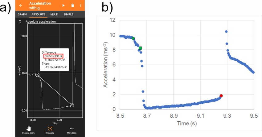
Educ. Sci. 2021, 11, 493                                                                                                      4 of 20

                           Figure 1. (a) Picture of the 3B-Scientific set-up. On the left there is the vertical guide, with the steel
                           ball release system on top and the ball arrival sensor (red circle) on the bottom. The time counter is
                           on the right. (b) Picture of the material used to exploit the Phyphox acoustic stopwatch. (c) Picture of
                           the material used to make the video of a falling tennis ball. The smartphone is fixed on a mini-tripod
                           on a chair. On the back, and in the smartphone screen, the bookshelf with the folding meter is visible.
                           (d) Picture of the sofa used for the experiment with the smartphone accelerometer, also showing the
                           vertical meter used to control the smartphone release height.

                                The determination of g from Equation (4) was also performed with smartphone-based
                           experiments, using a Huawei Y6 2019 and different methods.
                                The first method exploits the acoustic stopwatch of the app Phyphox, that deter-
                           mines the time interval between two sounds, with a nominal temporal resolution of 1 ms
                           (see Figure 1b). The falling body was a steel sphere with a 1.3 cm diameter, taken from a
                           famous magnetic construction toy, initially at rest on a metallic ruler protruding from the
                           shelf of a bookshelf. The initial height was measured with a wooden folding meter rule,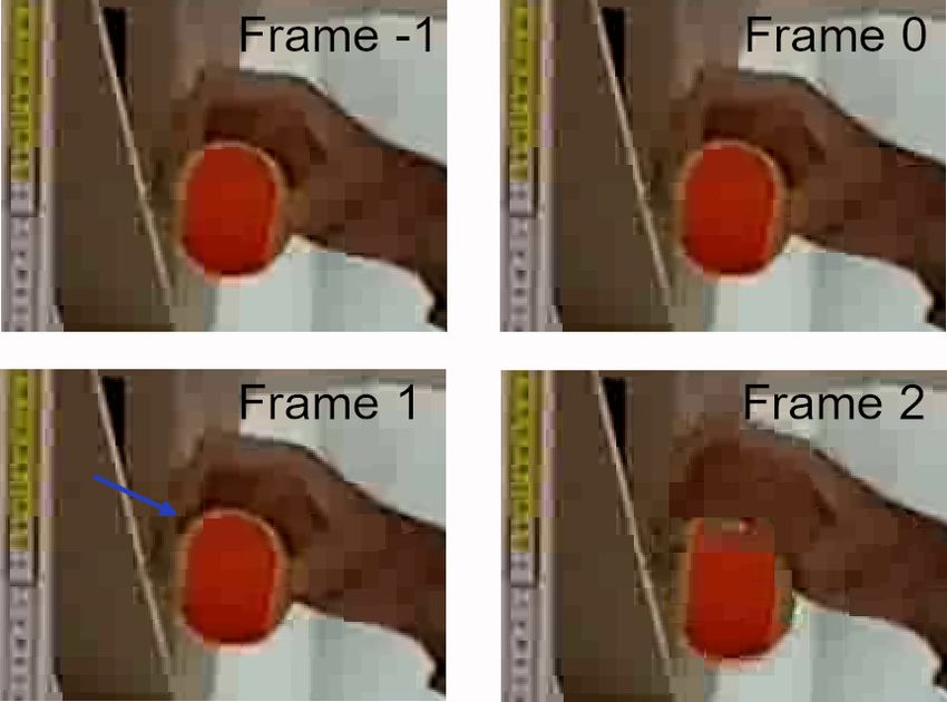
Educ. Sci. 2021, 11, 493                                                                                                  5 of 20

                           while the starting sound was generated by suddenly hitting the ruler with a pen, in order
                           to make it move along the horizontal direction. The stopping sound was instead generated
                           by the sphere impact with a metal box on the floor [22].
                                For the second method, we determined the falling time starting from the video of
                           the motion, made with the smartphone internal camera with the smartphone fixed to a
                           mini-tripod (see Figure 1c). The video (originally in 3gp format) was converted to mp4 by
                           using the free software Video to Video converter, from Media Converters, and opened with
                           the free software Tracker [24]. The necessity to easily see the falling object in the movie
                           lead us to use a tennis ball rather than the steel sphere which was too small. The ball was
                           held in hands, taking care to leave it falling without giving it any initial velocity and in the
                           fastest possible way. The determination of the falling time in this case is a bit tricky, as the
                           temporal sensitivity is limited by the video frame rate (30 Hz), leading to one frame every
                           33.3 ms. For this reason, the movie typically contains neither a frame showing the release
                           instant t0 nor the instant in which the ball hits the ground t f . The ball release instant t0
                           was determined by carefully looking at the video frame by frame, focusing the attention on
                           the few frames across the ball release (see Figure 2). We thus determined t0 as the average
                           value between the time of the last frame showing the ball being held by the hand (Frame 0
                           in Figure 2) and the time of the first frame showing the movement of the fingers to release
                           the ball (Frame 1 in Figure 2) .

                           Figure 2. Picture of the frames across the ball release. Frame −1 and Frame 0 are the last two frames
                           showing the ball held in the hand. Frame 1 show a space, evidenced by the blue arrow, between the
                           hand and the ball, indicating the hand opening and Frame 2 clearly show that the ball has been fully
                           released and is already moving.

                                In a similar way t f was determined as the average between the time of the last frame of
                           the falling motion and the following frame (already showing the ball after the bounce on the
                           ground). Both values lie in a time interval 33 ms wide, thus have a maximum uncertainty
                           of 16.5 ms, leading to a maximum error of 33 ms on their difference. A statistical√error
                           on t0 and t f was instead determined by dividing the maximum uncertainty by 3, as
                           expected for a uniformly distributed variable, and on ∆t f by adding the statistical errors in
                           quadrature, obtaining 13.5 ms.
Educ. Sci. 2021, 11, 493                                                                                                   6 of 20

                                 As a third method, we instead exploited the smartphone’s internal accelerometer, again
                           using Phyphox, which allows to measure the acceleration in the smartphone reference
                           system. In this experiment, the falling object is the smartphone itself, which is left to fall on
                           a soft body (a sofa in our case, see Figure 1d), starting from rest. When the smartphone
                           is in equilibrium (for example when it is held by the hand) the accelerometer basically
                           measures the force necessary to compensate its weight, thus providing an acceleration
                           measurement equal to g (if it is properly calibrated). When the smartphone is in free fall,
                           both the accelerometer and the smartphone experience the same acceleration, thus their
                           relative acceleration is zero. Thus, during the free fall, the acceleration measured by the
                           accelerometer suddenly reaches values close to 0 m/s2 . Finally, when the smartphone
                           reaches the sofa, a sharp acceleration increase is observed, followed by some peaks, due to
                           the acceleration given by the force exerted by the sofa (see Figure 3). The acquisition rate of
                           the accelerometer data is 200 Hz, leading to a nominal temporal resolution of 5.0 ms.
                                 Phyphox allows to save the accelerometer data to visualize them on the smartphone’s
                           screen and then to export them in ASCII. The falling time can be determined as the time
                           difference between the instant of acceleration increase due to the impact with the sofa (first
                           point showing a sudden acceleration increase) and the smartphone release instant.
                                 The falling time was determined both by visually selecting the beginning and final
                           instant of the motion from the Phyphox app from the smartphone screen (see Figure 3a)
                           and, for an accuracy test, with Microsoft Excel, after transfer of the saved ASCII file to a
                           notebook by email (see Figure 3b).

                           Figure 3. (a) Screenshot of the Phyphox accelerometer option, evidencing the acceleration decrease
                           after the smartphone release, followed by a quick acceleration increase after the impact with the sofa.
                           The first line of the white rectangle (evidenced by the red rectangle) contains the time differences
                           between t f and t0 as determined on the smartphone screen with the “Pick data” option. (b) The same
                           data plotted with Microsoft Excel. The green circle is the point corresponding to t0 as the time of
                           beginning of acceleration decrease, the green square is the point corresponding to the time of slope
                           increase of the acceleration decrease and the red circle is the point corresponding to t f .

                                For all these three methods, we determined the falling time for 5 different values of
                           the initial height, given by the height of 5 different shelves of the used bookshelf.
                                For the two methods with the highest nominal temporal resolution (acoustic stopwatch
                           and accelerometer) we also estimated the uncertainty on ∆t f by repeating the measurement
                           3 times.
                                The acceleration of gravity was determined with different experimental procedures of
                           progressively increasing complexity:
Educ. Sci. 2021, 11, 493 7 of 20
• From Equation (4) by using a single value of the falling time for each starting height.
In this case the g estimation is very easy but the uncertainty level of the obtained
value cannot be estimated (for all the three methods).
• From Equation (4) by using the average value of the falling time obtained, for each
starting height, by repeating the measurements three times (for acoustic stopwatch
and accelerometer methods). In this case g can be determined for each starting height
with an estimate of the error bar.
• From the best fit with Excel of the ∆t2f dependence on h, that is expected to be linear
with a slope 2/g. In this case the linearity of the dependence allows to evidence
the validity of Equation (4), thus demonstrating that the falling motion is uniformly
accelerated, but no error bar on the g value can be obtained [25](for all the three
methods when using single measurements of ∆t2f and, only for acoustic stopwatch
and accelerometer methods, when using the average values).
• From the best fit with a professional software (Origin 8) with Equation (4), fully
including the data error bars and thus obtaining the statistically correct uncertainty
on the g values (again for all the three methods when using single measurements
of ∆t2f and only for acoustic stopwatch and accelerometer methods when using the
average values).
As a final approach we exploited the video of the falling motion of the tennis ball
(acquired and processed as already described above) to extract the time dependence of
its position, thus determining the temporal law of the motion, exploiting the presence of
the side of the book shelf of a folding meter rule fixed with tape, used for the pixel–cm
conversion. The position of the ball in the different frames was extracted with Tracker.
We observed that the exposure time during the video results in a poorly defined ball
image when the velocity exceeds about 2 m/s, opening to possible errors of the automatic
object tracking option of the software (see Figure 4). We thus determined the position of
the ball during the free fall by manually selecting the central pixel of the frame region
containing the ball image. The presence of the meter in the filmed frames allows to perform
a pixel-length calibration with Tracker, thus converting the position in pixel in height in
meters. The ball radius (3.2 cm) was then subtracted in order to determine the height of the
bottom point. The uncertainty of each position is limited by the size of the pixels and is
about 0.5 cm.
Furthermore, in this case the data analysis has been performed at two different
complexity levels. The simplest one is based on a linear regression with Microsoft Excel of
the lost height dependence on (∆t)2 :
1
h − y(t) = g(∆t)2 (5)
2
The second one is instead based on a best fit of the original data with Equation (2)
and Origin.
In order to quantify the relative accuracy of the obtained g values we define the
following quantity:
| gm − gex |
RA% = 1 − · 100 (6)
gex
where gm is the experimentally determined value and gex the expected one.Educ. Sci. 2021, 11, 493 8 of 20
Figure 4. Pictures of four frames after the ball release evidencing the progressively less defined ball
image as the velocity increases. The time is measured by considering t = 0 s for Frame 1 of Figure 2,
while the velocity is determined by Tracker.
3. Results
3.1. Professional Set-Up
As a first step we present the results obtained by the 3B-Scientific set-up, in order to
have a benchmark for the simpler smartphone-based methods. In this case the system
counts the time starting from the release instant, thus t0 = 0 s and ∆t = t.
The dependence of the falling time on the initial height shows (see Figure 5) a smooth
increase, visually consistent with the expected square root dependence. The qualitative
agreement between the experimental data and the expected increase is even more striking
when looking at the height dependence of the squared falling time (see inset of Figure 5),
that shows a very clear linear increase.
The g value has been determined by a best-fit with Equation (4) performed with
Origin, that allows to obtain an excellent fit for g = (9.7660 ± 0.0045) ms−2 . This value
is very close to the expected value (9.8020 ms−2 ) calculated by the International Gravity
Equation [26], for a latitude Φ = 40.334 °N:
h i
g = 9.780327 1 + 0.0053024 sin2 (Φ) − 0.0000058 sin2 (2Φ) ms−2 (7)
The relative accuracy is thus very high (RA% = 99.6%), but the extremely small
statistical uncertainty on g (relative statistical uncertainty of only 0.046 %) allows to observe
that the best fit value is not consistent with the expected value within 3 standard deviations.
A possible explanation of this result is a slight, but systematic overestimation of the falling
time. We observe that an underestimation of the g value of 0.4%, as in the current case, can
be obtained for an overestimation of ∆t f of just 0.2%, thus below 1 ms in the investigated
height range. Overall, the capability of the professional system to determine g and to verify
that the falling motion is uniformly accelerated is excellent and the small lack of accuracy
can only be observed due to the excellent reproducibility of the falling time values.Educ. Sci. 2021, 11, 493 9 of 20
0.45
0.40
0.35
0.30
0.20
t (s)
0.25
0.15
f
0.20
(s )
2
0.10
2
0.15
f
t
0.05
0.10
0.00
0.05 0.0 0.2 0.4 0.6 0.8 1.0
h (m)
0.00
0.0 0.1 0.2 0.3 0.4 0.5 0.6 0.7 0.8 0.9 1.0
h (m)
Figure 5. Falling time dependence on the starting height for the steel ball used in the 3B-Scientific
set-up. The red line is the best fit curve with Equation (4). Inset: the same data re-plotted with t2f on
the vertical axis, evidencing a nice linear increase, expected for a uniformly accelerated fall.
Similar very high accuracy and small statistical errors can be typically obtained
with other set-up often used in teaching laboratories, like for example spark timer-based
systems [20].
3.2. Smartphone Based Falling Time vs. Starting Height Dependence
3.2.1. Single Measurement
As the initial step in the evaluation of the smartphone-based methods we started by
performing a single measurement of the falling time for each of the five starting heights.
The values obtained from the motion video and the acoustic stopwatch are reported in
the second and third column of Table 1, while the values obtained with the accelerometer
are reported in the fourth and fifth column.
Concerning the falling time determined from the accelerometer data we observe that
(see Figures 3 and 6a) the final impact always determined a sudden acceleration increase,
thus making easy the determination of the final instant in correspondence of the last
point before the acceleration increase. On the contrary, the initial acceleration decrease
is much smoother (see Figures 3b and 6b) and it is thus not obvious which is the instant
corresponding to the free fall beginning. We thus initially assumed that the smartphone
release instant coincides with the instant of beginning of the acceleration decrease (green
dot in Figures 3b and 6b, corresponding to the last point before the initial acceleration
decrease), but we observed that this choice leads to systematically overestimate the falling
time of about 30–50 ms (with respect to the value calculated from Equation (2) with g =
9.8020 ms−2 ).
Moreover, we observed that if the smartphone is released by suspending it with a
wire and cutting the wire with scissors [6], the acceleration decrease is much faster and the
falling time is very close to the expected one (see black line in Figure 6a). Finally we show
that, in the case of a manual smartphone release, the initial acceleration decrease is gradual
in the first 30–50 ms, and then a clear slope increase is observed. In some cases, after a
gradual decrease, a small peak is observed after 30–50 ms, followed by a fast decrease.
Moreover, the release instant for the cutting wire method almost coincides with the instant
of the slope increase or of the peak (see Figure 6a).Educ. Sci. 2021, 11, 493 10 of 20
10 h=175.5 cm
a) b) 10.0
Wire
5 7.5
0 5.0
10 h=150.0 cm 2.5
Acceleration (ms )
Acceleration (ms )
-2
-2
5 0.0
0 10.0
Manual peak
10 h=105.0 cm 7.5
5 5.0
0 2.5
10 h=79.5 cm
0.0
5 10.0
Manual smooth
0 7.5
10 h=47.3 cm 5.0
5 2.5
0 0.0
0.0 0.2 0.4 0.6 0.8 1.0 1.2 0.0 0.1 0.2 0.3 0.4
Time (s) Time (s)
Figure 6. (a) Accelerometer data for different starting height, evidencing the progressive increase of
the falling time. The signals are horizontally aligned to the release instant. (b) Comparison of the
acceleration signals obtained for h = 175.5 cm for manual release, with smooth decrease (red line)
and for decrease followed by a peak (blue line), and for release by cutting a suspension wire (black
line). The signals have been aligned to the final instant. The dotted green line demonstrates the good
correspondence between the time of beginning of acceleration decrease for manual release (green
dot), while the red dotted line demonstrates the correspondence between the release time when
cutting the wire and the time of acceleration peak or slope increase (green square).
Overall, we concluded that the initial gradual acceleration decrease, or the decrease
followed by a peak, is relative to the time interval in which the smartphone starts to move,
but it is still in contact with the hand. The real free fall starts in correspondence of the slope
increase of the acceleration decrease, that was thus considered as the starting instant (green
square in Figures 3b and 6b, corresponding to the last point before the slope increase of the
acceleration decrease).
Even if the signal is obtained by suspending the smartphone and cutting the wire
is easier to analyze, we find this advantage smaller than the complexity increase due to
the creation of a suspension system that allows a good alignment with the meter and an
easy repetition of the measurements. We thus preferred to use the straightforward manual
release procedure, making care in the falling time extraction.
Table 1. Values of the falling time ∆t f obtained from a single measurement with acoustic stopwatch,
accelerometer and video analysis techniques for 5 different values of the starting height h. The
expected value of ∆t f is also reported for comparison.
Height Single Time (ms) Expec.
(m) Video Acous. Acc. vis. Acc. Exc. Time (ms)
0.473 300 321 304 299 311
0.795 400 411 390 401 403
1.050 433 469 482 477 463
1.500 567 560 562 553 553
1.755 600 614 613 603 598
As already noticed the difficult part of an accurate determination of g starting from
the falling time values is given by the requirement of determining the small values of ∆t f
with a small error. As ∆t f increases with h it is reasonable to expect that a good strategy
to minimize the relative error on ∆t f will be the increase of h. For this reason, we start
the presentation and discussion from the results based on the ∆t f values obtained for the
maximum available height (h = 1.755 m).
We initially observe that the two values obtained by the acoustic stopwatch and the
accelerometer (extracted from the smartphone screen) are almost identical, with just 1 ms
of difference. On the contrary the value extracted from the accelerometer and Excel isEduc. Sci. 2021, 11, 493 11 of 20
slightly smaller, even if the difference is of only about 10 ms, corresponding to just two
measurement steps. The value extracted from the video, that can change only for multiples
of 33 ms, is instead consistent with all the previous 3 values.
Despite this promising similarity between different methods, we observe that the
obtained values are higher than the expected value, with differences between 2 ms and
16 ms. Even if this difference looks small, providing a relative error below 2.7%, the inverse
proportionality between g and the squared falling time leads to very evident differences
between the obtained values (see Figure 7a), spanning from 9.33 ms−2 (acoustic stopwatch)
to 9.75 ms−2 (video).
11.5 11.5
Acoustic Acoustic
a) Accelerometer
b) Accelerometer
11.0 visual
11.0 visual
Accelerometer Accelerometer
exc exc
10.5 10.5
Video
10.0 10.0
g (ms )
g (ms )
-2
-2
9.5 9.5
9.0 9.0
8.5 8.5
8.0 8.0
0.4 0.6 0.8 1.0 1.2 1.4 1.6 1.8 2.0 0.4 0.6 0.8 1.0 1.2 1.4 1.6 1.8 2.0
Starting height (m) Starting height (m)
Figure 7. (a) Values of g obtained from a single measurement of the falling time for 5 different
starting heights determined with the Phyphox acoustic stopwatch, with the accelerometer and from
the motion video. The horizontal line demonstrates the expected value. (b) Values of g obtained
from the average value of 3 measurements of ∆t f for 5 different starting heights, with the Phyphox
acoustic stopwatch and with the accelerometer. The horizontal line demonstrates the expected value.
This first set of measurements suggests a general tendency of all the methods of
overestimating the falling time value and, concerning the accelerometer data, a further
overestimation of the values directly extracted with Phyphox from the smartphone screen
with respect to the one determined from Excel.
In order to probe the generality of this result, we repeated the measurement for four
further values of the starting height (see Table 1). The obtained results allow to observe that
the ∆t f values obtained with the acoustic stopwatch are again always slightly overestimated
(between 6 ms and 10 ms), with a relative error between 1.2% for h = 1.50 ms and about
3% for h = 0.473 m. Moreover the ∆t f values obtained with the internal accelerometer and
directly extracted form the smartphone screen are again always slightly larger (between
5 ms and 9 ms) than the values extracted with Excel. As a consequence, the g values
obtained from the ∆t f values measured by the acoustic stopwatch are systematically lower
than the expected value, with values between 9.18 ms−2 and 9.57 ms−2 (see Figure 7a).
The point to point variation of the values extracted with the accelerometer data is instead
higher, even if in a couple of cases (data extracted with Excel for h ≥ 1.50 m) the g value is
very close to the expected one.
Overall, these further data confirm that the acoustic stopwatch has a systematic
tendency to overestimate the falling time, thus underestimating g. On the contrary, the
data obtained from the accelerometer, even if a bit more scattered, seems to sometimes
allow a good evaluation of the g value.
Anyway, for both methods, the presence of a single value of ∆t f does not allow to
estimate its error bar and thus an error bar for g, preventing any conclusion about the
consistency between the obtained values and the expected ones beyond a qualitative
comparison of the two values.
Concerning the g values obtained from the video of the free fall (see Figure 7a) we
observe that the potentialities of this technique are clearly limited by the coarse time
scale, that is intrinsically limited to variations in steps of 33 ms. This results in a coarse
determination of ∆t f and, as a direct consequence, in highly scattered values of g that varyEduc. Sci. 2021, 11, 493 12 of 20
in the range between 9.34 ms−2 and 11.1 ms−2 without any regular dependence on h. A
unique relevant advantage of this technique is that its poor temporal sensitivity allows to
use the time step as uncertainty on the ∆t f values, thus allowing to estimate an error bar
for g even with a single ∆t f measurement.
The maximum error bar on ∆t f is fixed to 33 ms, thus the relative error on ∆t f
decreases from about 10% for h = 0.473 m to about 5% for h = 1.755 m, leading to a maximum
(statistical) error on g decreasing from 2.4 ms−2 (0.8 ms−2 ) to 1.1 ms−2 (0.4 ms−2 ). The
best g estimate is thus obtained for the maximum value of h and it is g = 9.8 ± 1.1 ms−2
(g = 9.8 ± 0.4 ms−2 if the statistical error is considered). We observe anyway that this best
performance is positively affected by a casualty of the almost perfect coincidence of the
measured ∆t f with the expected one. In other cases, the interplay between an increasing
relative error on ∆t f and less lucky correspondence of the expected time with the possible
ones results in much higher uncertainty bar. For example, for h = 1.05 m the obtained
value is g = 11.2 ± 1.7 ms−2 (g = 11.2 ± 0.6 ms−2 if the statistical error is considered) that is
neither accurate nor precise.
3.2.2. Average of Many Measurements
As a next step we decided to explore in further detail the potentiality of the two
methods with the better nominal sensitivity on ∆t f , thus the acoustic stopwatch and the
accelerometer ones, focusing our attention on the estimation of a reasonable error bar on
the ∆t f values while preserving the overall simplicity of the experiment.
We thus repeated all the ∆t f measurements two more times for each starting height,
determining the best estimate of ∆t f as average and of the maximum uncertainty as the
semi-dispersion of the three measured values. The obtained values (see Table 2) allow
to observe a generally good reproducibility of the ∆t f values obtained with the acoustic
stopwatch, with semidispersion between 1.0 ms and about 10 ms, even if the values are
again overestimated for four of the five investigated values of h. As a consequence, with the
only exception of the value obtained for h = 1.755 m, the obtained g values (see Figure 7b)
are systematically lower than the expected value and, more importantly, not compatible
with it within the error bar. The average value of g for h ≥ 0.795 m is g = 9.5 ± 0.2 ms−2
when maximum errors are considered (g = 9.50 ± 0.07 ms−2 for statistical errors).
On the contrary, the data obtained from the accelerometer and directly determined
from the smartphone screen show a slightly larger semidispersion of about 15 ms, but
the average values of ∆t f is consistent within the error with the expected one for all the h
values. As a consequence, also the corresponding g values are comparable with each other,
with an average value of g = 9.9 ± 0.3 ms−2 , and compatible with the expected one within
the error bar (see Figure 7b). When statistical errors are used, rather than the maximum
errors, we find g = 9.91 ± 0.10 ms−2 , that is compatible with the correct value within one
standard deviation.
Table 2. Average values and corresponding maximum error bar of ∆t f for both acoustic stopwatch
and accelerometer techniques, obtained by performing 3 independent measurements of ∆t f for each
value of h. The expected value of ∆t f is also reported for comparison.
Height Average Time (ms) Expec.
(m) Acous. Acc. vis. Acc. Exc. Time (ms)
0.473 329 ± 10 308 ± 3 308 ± 10 311
0.795 410.3 ± 1.0 392 ± 13 402 ± 3 403
1.050 479 ± 10 464 ± 15 461 ± 13 463
1.500 559.0 ± 1.0 556 ± 7 548 ± 5 553
1.755 598 ± 13 599 ± 16 598 ± 5 598Educ. Sci. 2021, 11, 493 13 of 20
The data obtained from the accelerometer and Excel shows a semidispersion between
3 ms and 13 ms and are again consistent with the expected value for all the investigated
heights. As a consequence also the corresponding g values are consistent within the error bar
with the expected value (see Figure 7b). By estimating the average value of all the obtained g
values we find g = 9.9 ± 0.1 ms−2 , that becomes g = 9.90 ± 0.03 ms−2 when statistical errors
are considered (compatible with the expected value within 3 standard deviations).
3.2.3. Comparison of the Methods
Coming to a comparison of the cost/result balance of the three methods we observe
that the potentiality of use of the video is clearly limited by the coarse determination of
∆t f , leading to a rather unpredictable accuracy and a large error bar on g. In the best
case we obtained a relative accuracy RA% as high as 99.5%, but with a relative error bar
of 11%. In the worst case the relative accuracy was only 86%, with a relative error above
17%. Overall, this technique is in general not very precise, potentially not particularly
accurate and, in addition, it is not immediate, as it requires several steps (making the
video, transfer to the computer, file format conversion, extraction with Traker and paying
attention to determine the starting and finish frame of the motion). The only reasonable
use of a similar experiment is to provide an example of unconventional use of a video
made by a smartphone for the determination of a reasonable value of a physical quantity,
but certainly it is not the best choice as easy and accurate method for the g determination.
Concerning the acoustic stopwatch, it has the enormous quality of being the only
method that allows to directly measure the falling time, without requiring any additional
step after the measurement. The required set-up is very simple and the time needed for the
measure on the scale of few minutes.
However, the method has a systematic tendency to overestimate the falling time
values [27], thus underestimating g. The reproducibility of the ∆t f values is instead gen-
erally very good, thus allowing a very precise measurement (average statistical error
as low as 0.7%), but unfortunately the technique is not the most accurate, with typical
RA% ≈ 95%. Overall, if this accuracy level is considered acceptable, this method with a
single measurement is certainly the best choice.
We also observe that the time cost of repeating the measurements in order to allow
the addition of the error bar is extremely limited, and the accuracy of the technique seems
to increase with increasing h, thus suggesting to use the average of many measurements
approach for h ≥ 1.50 m as the best cost/results option, allowing to reach RA% ≥ 98%.
Concerning the method exploiting the internal accelerometer, used with single mea-
surement and data extraction from the smartphone screen, we found a relative accuracy
similar to the acoustic stopwatch one for h ≥ 1.50 m, and a comparable complexity. How-
ever in this case the accuracy is limited by the small errors on ∆t f (typically below 10 ms if
care is taken in selecting the start and finish points on the screen) due to the use of direct
∆t f extraction from the smartphone screen. The addition of the data export step and ∆t f
extraction with Excel is rewarded by an accuracy increase above 98.4 % for h ≥ 1.50 m.
When the repetition of measurements is added, the technique allows to obtain g
values compatible within the error to the expected one for any h value. It is interesting to
observe that, even when directly extracting the data from the smartphone screen, very high
RA% ≥ 99% can be obtained for h ≥ 1.05 m. No advantages are observed instead when
extracting the data with Excel, showing that the errors induced by direct extraction of ∆t f
from the screen average out when repeating the measurements just three times.
Overall the average of many measurements option with direct data extraction is the
best choice in terms of costs/results ratio, demonstrating amazingly high relative accuracy
and overall simple and fast execution.
3.3. Investigation of the Nature of the Motion
After the establishment of the potentiality of the acoustic stopwatch, accelerometer
and video analysis methods to determine g starting from Equation (4), a limited number ofEduc. Sci. 2021, 11, 493 14 of 20
measurements and a simple error analysis, we investigated how far these methods can go
in the physical analysis of the free fall.
Even if these further experiments can probably go beyond the level expected for high
school students, they could be suitable for experiments at university level, or for hybrid
courses organized by universities for high school students.
A very instructive aspect would be the experimental test of the validity of Equation (3),
that would allow to directly probe the validity of the assumptions on which the solution
is based (negligible viscous friction and constant gravity acceleration) and to show to the
students how a theoretical prediction can be experimentally validated.
In order to obtain this result, we analyzed, for each technique, the falling time depen-
dence on the starting height, basically reproducing the experiment performed with the
3B-Scientific set-up.
Again we followed two experimental procedures, measuring ∆t f just once for each
starting height (thus performing five measurements of ∆t f in total, one for each of the
five different investigated heights), or measuring it three times for each height and using
the average ∆t f values (requiring three measurements of ∆t f for each height, thus 15
measurements overall).
In both cases we performed two different analysis, starting from a simple one based
on Excel and then moving to a professional best fit performed with Origin.
The simple analysis is performed by plotting with Excel the squared ∆t f values as a
function of h that, according to Equation (3), should show a linear dependence with slope
2/g. We first analyzed the data obtained by a single ∆t f measure for each h, observing
(see Figure 8), for all the investigated methods, a visually good linear increase, thus qualita-
tively confirming the motion with uniform acceleration. A simple linear regression allows
to determine the best value of the slope and, thus, the best estimate of g. Even if Excel
does not estimate any error bar for the best fit parameters, the regression on five points
allows to compensate the effects of scattered values of ∆t f on the value of g, thus leading
to best g estimates most of the time quite close to the expected values. In particular, the
relative accuracy of the g value obtained from the video (see Figure 8a) is RA% = 99.5%,
and also the values obtained by using the accelerometer differ from the expected value of
less than 4% (RA% = 96.4% for the ∆t f values directly extracted from the screen and RA%
= 99.8% when the ∆t f extracted with Excel are used). On the contrary the systematic, and
rather regular, overestimation of ∆t f with the acoustic chronometer leads in this case to an
underestimated g value (9.43 ms−2 , thus RA% = 96.2%).
When the average ∆t f values are used, the additional averaging of the point to point
fluctuations further improves the accuracy for the accelerometer methods above 99%
(g = 9.80 ms−2 for the visual method, and g = 9.85 ms−2 with Excel method). The value
obtained with the acoustic stopwatch data is instead still underestimated, even if with
slightly improved accuracy (g = 9.57 ms−2 , thus RA% = 97.6%).
The absence of an error bar of course technically prevents to evaluate the real compati-
bility between the obtained values and the expected one but, at an introductory level, such
a good accuracy easily allows to qualitatively agree that the values are very close to the
expected one.
In order to add a proper error bar to the obtained g values, the data have been
re-analyzed with Origin and directly fitting them to the following equation:
s
2h
∆t f = (8)
g
The obtained best fit values of g coincide with the ones obtained by Excel, thus
allowing to limit the discussion to the differences in the g error bars.
The data scattering from the video leads to a maximum (statistical) error on g of
0.9 ms−2 (0.31 ms−2 ) confirming the lack of precision of the method. On the contrary
the acoustic stopwatch is confirmed as the method with higher precision, evidenced
by a maximum (statistical) error on g of only 0.2 ms−2 (0.066 ms−2 ) when the singleEduc. Sci. 2021, 11, 493 15 of 20
∆t f measurements are used and 0.13 ms−2 (0.044 ms−2 ) when average values are used.
Finally the data from the accelerometer and extracted from the screen lead to a maximum
(statistical) error on g of 0.6 ms−2 (0.22 ms−2 ) when the single ∆t f measurements are
used and 0.2 ms−2 (0.070 ms−2 ) when average values are used. When the step of data
extraction with Excel is added the data quality is slightly improved, reducing the maximum
(statistical) error on g of 0.5 ms−2 (0.17 ms−2 ) when the single ∆t f measurement is used
and 0.12 ms−2 (0.040 ms−2 ) when average values are used.
3.3.1. Comparison of the Methods
All the four methods allow to evidence the expected square root dependence of ∆t f
on h, basically confirming the differences in terms of accuracy and precision already found
in Section 3.2.3.
Concerning the video method, the averaging effect of a single fit on many points
allows to reach a good accuracy, but the starting high data scattering makes it the one with
the worst precision.
The acoustic stopwatch method turns out to have the worst accuracy due to the
systematic overestimation of the falling times, but is the most precise. This makes it again
competitive with the accelerometer with visual data extraction when single measurements
of ∆t f are made in terms of final accuracy and overall suitable for easily demonstrate the
validity of Equation (3).
When high accuracy is desired, the average of more ∆t f is required and the most
powerful methods are without any doubt the ones exploiting the accelerometer, allowing
to reach accuracy above 99% with relative maximum (statistical) error bar down to only
1.2% (0.4 %).
Figure 8. Starting height dependence of the squared falling time ∆t2f obtained from a single measure-
ment with the video (a), acoustic stopwatch (b), accelerometer and direct extraction from the screen
(c) and with Excel (d). The dotted lines are the best regression line determined by Excel.Educ. Sci. 2021, 11, 493 16 of 20
3.4. Motion Temporal Law
In this last section we discuss the possibility to use the video of the falling motion of
the tennis ball to extract the temporal dependence of its height, thus directly determining
the position-time dependence.
The time dependence of the ball position extracted with Tracker clearly shows
(see Figure 9a) the progressive increase of the covered distance between consecutive frames
(thus for a fixed time interval), fully consistent with an accelerated motion. It is also evident
that the picture is very similar to the ones typically shown on text books but determined
with typically inaccessible instrumentation (like the photographs under stroboscopic flash
light). Even if only qualitative, this first result is extremely interesting, because it demon-
strates that the combination between a smartphone, a free software and a bit of time can
allow anybody curious and patient enough to reproduce the results typically requiring
professional instrumentation.
The time dependence of the ball height is shown in Figure 9b and demonstrates a
downward convex curved dependence, qualitatively consistent with the expected parabolic
dependence of Equation (2) (in this set of data the t = 0 s point is relative to the last frame
in which the hand holds the ball, thus Frame 0 in Figure 2).
In order to better visualize the qualitative agreement between the expected depen-
dence and the experimental data, we also plotted the lost height at any time as a function
of ∆t2 (see Figure 9c), which shows a smooth increase, qualitatively consistent with the
linear dependence expected from Equation (5).
In order to quantitatively analyze the data we started again from an Excel-based
analysis of the linearized dependence of the lost height, providing in this case a slope g/2.
By performing a linear regression fixing the intercept at 0 and t0 = 16.5 ms (average
between t = 0 s of Frame 0 and t = 33 ms of Frame 1) we obtained g = 9.50 ms−2 . We also
investigated the importance of a correct knowledge of t0 , that is not directly measured but
only estimated as average value between the two extreme values t = 0 s and t = 33 ms, by
repeating the analysis for the two extreme values. By fixing t0 = 0 s we find g = 8.87 ms−2 ,
that is macroscopically underestimated, while for t0 = 33 ms we find g = 10.19 ms−2 , that
is on the contrary overestimated. This result demonstrates that the g value is strongly
affected by the value of t0 , that unfortunately cannot be directly measured, leading to
potentially widely scattered g values despite the availability of a data set with 19 measured
points, by far the richest one among all the investigated techniques, and the use of great
care to determine in the best possible way the two frames across the ball release, the
position of the ball at each frame and the pixel-length calibration. Differences between the
estimated t0 and the real value can determine g variations up to 0.7 ms−2 resulting in a
rather unpredictable accuracy (down to 90% even without making any error).
In addition, we also simulated a situation in which an error of just one frame is made
in determining the last frame in which the ball is at rest, obtaining g = 8.29 ms−2 when t0 is
placed one frame back and g = 10.94 ms−2 when it is placed one frame forward, further
reducing the accuracy down to about 84%. This result clearly demonstrates that the careful
determination of the correct frames across the ball release is fundamental in order to have
chances to adequately quantify g.Educ. Sci. 2021, 11, 493 17 of 20
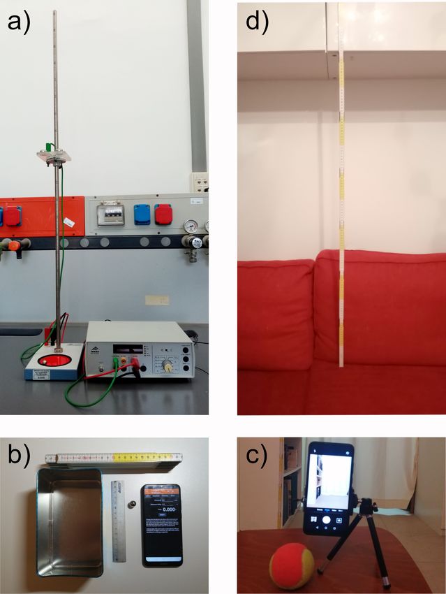
Figure 9. (a) Picture of the library used to extract the motion temporal law from the video. The pink
lines are the axis of the reference system, while the black line is the calibration stick built exploiting
the folding meter on the side of the library. The full blue dots represent the positions of the ball
extracted from the different frames of the video between the ball release and the bounce on the floor.
(b) Time dependence of the tennis ball height extracted from the motion video for both the data
originally extracted with Tracker (full black dots) and the data with distortion correction (open blue
dots). The lines are the best-fit curves with Equation (2). (c) Lost height dependence on the squared
time, evidencing the expected linear increase. The line is a linear regression line obtained with Excel.
(d) Difference between the ball height extracted with Tracker and the ones measured from the meter
image in the video (full black dots) and best-fit curve (red line). The open black dots represent the
difference between the distortion corrected heights and the best-fit ones.
We thus decided to investigate in further detail the g dependence on t0 , leaving the
Excel-based data analysis and moving to a professional analysis with Origin. In this case
we directly used the original data and we adapted them, in the sense of minimum Chi
squared, with Equation (2).Educ. Sci. 2021, 11, 493 18 of 20
The best fit was initially obtained by fixing t0 to 16.5 ms, the initial height to the
measured one, and the initial velocity to 0 and allowed to obtain g = 9.47 ± 0.03 ms−2 . The
best g estimate almost coincides with the one determined with Excel, but the addition of
the error bar demonstrates that this value is clearly not consistent with the expected value.
A slightly improved fit is obtained by allowing the variation of t0 (best fit value
t0 = 12 ± 2 ms, thus actually between Frame 0 and Frame 1, as expected) but for
g = 9.32 ± 0.08 ms−2 , that is even farther from the correct value. This disagreement thus
demonstrates that something else is still preventing a good agreement between the data
and the model.
As a last step we thus checked the correctness of the frame-time and the pixel-length
correspondence.
The video frame rate has been checked by making a video of a running chronometer
and observing that actually 30 frames are always present in 1 second. Thus, each frame is
effectively recorded every 33 ms, as assumed.
The pixel-length calibration has been instead checked by exploiting the presence of
the meter in the video and determining the pixels corresponding to the meter change of
color (from yellow to white and viceversa, every 10 cm). We thus compared the height
values obtained from the pixel-position calibration (hcal ) with the corresponding values
read on the meter (hreal ), observing (see Figure 9d) a clear systematic difference hcal − hreal
down to about −4 cm for h ≈ 1 m (the two values at h = 2.000 m and h = 0.000 m are the
same by construction of the calibration stick).
We thus adapted the dependence of the measured height hcal on the real one hreal with
a quadratic function, and we then used the best fit curve to calculate the correct height
values for each frame of the video. The differences between the corrected heights and
the ones calculated from the best fit are always below 0.5 cm, and are correctly randomly
distributed around 0 (see Figure 9d).
By performing a best fit with Equation (2) of the temporal dependence of the corrected
heigth we finally obtained g = 9.63 ± 0.07 ms−2 .
This last g value is finally compatible within three standard deviations with the
expected value, and demonstrates a relative accuracy RA% = 98.2% with a relative statistical
uncertainty of 0.7%.
Basically the same result (g = 9.61 ± 0.08 ms−2 ) can be obtained by performing a best
fit with Equation (1), fixing t0 = 16.5 ms and leaving v0y as free parameter (best fit value
v0y = (−0.115 ± 0.018) ms−1 ).
We can thus conclude that the extraction of the motion temporal law starting from
the frames of the video is surely possible. However, it cannot be expected to extract
quantitatively correct values of g without the image spatial distortion correction and the
possibility to perform a best fit more complex than a regression of the linearized data.
Overall, also this approach is potentially very interesting, as it is the only one that directly
gives access to the possibility to fully analyze the motion (i.e., the variation with time of the
position) but the complexity of the whole procedure is likely above the level accessible to
students/curious individually working at home without a professional supervision.
4. Conclusions
In conclusion, we quantitatively compared several different methods to determine g
with smartphone-based experiments.
We demonstrated that the determination of g from the falling time measurement from
a single known height, that just needs one measurement and a standard calculator, is in
general possible with all the tested methods.
Anyway, the falling time extraction from the video of the motion was evaluated
too complex for the results that it allows to obtain, with low precision and rather unpre-
dictable accuracy.Educ. Sci. 2021, 11, 493 19 of 20
On the contrary, reasonable accuracy (RA% ≈ 95%) was obtained when using the
Phyphox acoustic stopwatch and the internal accelerometer with direct data export, for
starting height of at least 1.50 m.
For the accelerometer method, the addition of data export to Excel allows better
accuracy with single measurement (above 98%) for starting height of at least 1.50 m, but of
course increased complexity.
With the addition of two further measurements, allowing to determine the aver-
age falling time, an accuracy increase is observed for the acoustic stopwatch (98%) and
h ≥ 1.50 m, while the use of the accelerometer with direct data extraction allows to reach
higher accuracy (above 99 %) for every starting height, and can thus be suggested as best
compromise between high accuracy and easy operation. The use of average measurement
and data extraction with Excel provides the same accuracy, but it is more complex, thus it
is not recommended.
Moving to methods requiring spreadsheet software for data analysis, to verify the
actual nature of the motion, i.e., uniformly accelerated, again all the methods provide
visually good data. When accuracy is considered, the best compromise between accuracy
and complexity is provided by the use of the accelerometer with direct data extraction and
average of many measurements.
Finally, we demonstrated that the combination of the video of the free fall motion
and video analysis with Tracker allows to determine the motion temporal law with a
qualitative agreement with the expected one. However, beyond the general complexity of
the procedure for the determination properly calibrated ball position as a function of time,
the method was demonstrated not reliable to quantitatively obtain the g value without
professional data analysis techniques. The g value extracted from an Excel data analysis
strongly depends on the initial instant value, leading to a rather poor accuracy (down to
about 90%) even without making any error. In addition, if an error of just one frame is
made in the determination of the release time the accuracy can decrease down to 85 %.
A proper correction of the image distortion and the use of professional fitting program
allows to reach accuracy of about 98%, that remains lower than the much simpler techniques
based on the falling time dependence on the starting height.
Among all the methods and experimental procedures, the best choice is given by the
g determination from the falling time measurement from a known starting height, the use
of the internal accelerometer with direct data extraction and average of three falling time
measurements. This technique is overall simple, fast, and does not require any external
software of data processing, except a standard calculator. The only aspect that requires
care is the fast release of the smartphone and a bit of attention in correctly determining
the starting and final times from the acceleration temporal dependence. While the 3B-
Scientific set-up is unbeatable in terms of absolute accuracy and versatility in performing
many falling time measurements easily and quickly, it is interesting to observe that the
best smartphone-based method allows to obtain overall similar performances in terms of
relative accuracy (99% against 99.6%) with a relative statistical uncertainty of just 1% (20
times higher than the 3B-Scientific one).
Funding: This research received no external funding.
Data Availability Statement: The data in this manuscript can be shared with interested people by
directly contacting the author.
Acknowledgments: Maria Luisa De Giorgi is acknowledged for useful discussions along all the paper
preparation, my two sons Raimondo (12 years old) and Filippo (8 years old) are acknowledged for
repeating part of the measurements to check the suitability of the different methods to be reproduced.
Conflicts of Interest: The author declares no conflict of interest.You can also read