Quantum field theory on global anti-de Sitter space-time with Robin boundary conditions
←
→
Page content transcription
If your browser does not render page correctly, please read the page content below
Quantum field theory on global anti-de Sitter
                                         space-time with Robin boundary conditions
                                                      Thomas Morley
arXiv:2004.02704v2 [gr-qc] 10 Oct 2020

                                                      Consortium for Fundamental Physics, School of Mathematics and Statistics,
                                                      Hicks Building, Hounsfield Road, Sheffield. S3 7RH United Kingdom
                                                      E-mail: TMMorley1@sheffield.ac.uk

                                                      Peter Taylor
                                                      Centre for Astrophysics and Relativity, School of Mathematical Sciences,
                                                      Dublin City University, Glasnevin, Dublin 9, Ireland
                                                      E-mail: Peter.Taylor@dcu.ie

                                                      Elizabeth Winstanley
                                                      Consortium for Fundamental Physics, School of Mathematics and Statistics,
                                                      Hicks Building, Hounsfield Road, Sheffield. S3 7RH United Kingdom
                                                      E-mail: E.Winstanley@sheffield.ac.uk

                                                      Abstract. We compute the vacuum polarization for a massless, conformally coupled
                                                      scalar field on the covering space of global, four-dimensional, anti-de Sitter space-time.
                                                      Since anti-de Sitter space is not globally hyperbolic, boundary conditions must be
                                                      applied to the scalar field. We consider general Robin (mixed) boundary conditions
                                                      for which the classical evolution of the field is well-defined and stable. The vacuum
                                                      expectation value of the square of the field is not constant unless either Dirichlet or
                                                      Neumann boundary conditions are applied. We also compute the thermal expectation
                                                      value of the square of the field. For Dirichlet boundary conditions, both thermal and
                                                      vacuum expectation values approach the same well-known limit on the space-time
                                                      boundary. For all other Robin boundary conditions (including Neumann boundary
                                                      conditions), the vacuum and thermal expectation values have the same limit on the
                                                      space-time boundary, but this limit does not equal that in the Dirichlet case.

                                                      PACS numbers: 04.62.+v

                                         Keywords: anti-de Sitter space-time, vacuum polarization, quantum field theory in
                                         curved space-time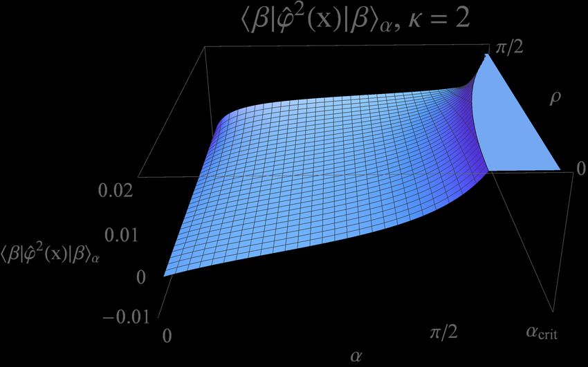
Quantum field theory on global anti-de Sitter space with Robin boundary conditions         2

1. Introduction

Quantum field theory (QFT) on anti-de Sitter (AdS) space-time has been the subject of
considerable attention owing to its role in the holographic principle and string theory,
particularly within the context of the AdS/CFT (conformal field theory) correspondence
(see for example [1] for a review). QFT on AdS is particularly rich, with a plethora of
possibilities to consider. As on any space-time, one can study a variety of bosonic [2–16]
and fermionic [4,11,17–24] quantum fields, and different quantum states, including static
vacuum states [4, 6, 7, 9, 11, 16, 19], static thermal states [2, 4, 18, 20, 21] and rotating
states [18, 25].
     Let us now consider the simplest possible quantum field, namely a massless,
conformally coupled scalar field. Even in this simplified model, there are many variations
to consider. First of all, the properties of the QFT of the scalar field depend on whether
one considers global AdS [2,4–6,9,11,15,16] or the Poincaré patch PAdS [12–14,26–28],
the latter being particularly relevant in the context of the AdS/CFT correspondence.
In both cases, the fact that AdS is not a globally hyperbolic space-time means that, in
order to have a well-defined QFT, appropriate boundary conditions must be applied to
the field at null infinity, which is a time-like surface [5, 13–15, 29–32].
     The simplest boundary conditions are either Dirichlet [2, 4, 5, 16] (where the field
vanishes on the boundary) or Neumann [2, 5] (where the normal derivative of the
field vanishes on the boundary). In [5] a third possibility is also studied, namely
“transparent” boundary conditions, which we do not consider further in this paper.
The advantage of working with either Dirichlet or Neumann boundary conditions is that
the vacuum Green’s function respects the maximal symmetry of the background AdS
space-time [3, 5], which enables renormalized vacuum expectation values to be derived
in closed form [2, 4, 16] and analytic expressions for renormalized thermal expectation
values can be found in terms of infinite sums of special functions [2, 4].
     However, Dirichlet and Neumann boundary conditions are not the only possibilities
leading to well-defined dynamics for a classical scalar field [33]. For example, one can
also consider Robin (or mixed) boundary conditions, in which a linear combination of the
field and its normal derivative vanish on the boundary [31, 34], or Wentzell boundary
conditions [14]. In the AdS/CFT correspondence, Robin boundary conditions for a
bulk quantum scalar field have been extensively studied (see [35–44] for an incomplete
selection of references on this topic), and correspond to multi-trace deformations of the
dual CFT.
     In this paper, we focus on the role the boundary conditions play for both vacuum
and thermal states of a massless, conformally coupled scalar field on the covering space
of global AdS in four space-time dimensions. Some of the interesting questions arising
in this context are:
 (i) Are general Robin boundary conditions physically valid?
(ii) Are vacuum and thermal states Hadamard for general Robin boundary conditions?
Quantum field theory on global anti-de Sitter space with Robin boundary conditions         3

(iii) Do the propagators for vacuum and thermal states respect the AdS symmetries for
      all Robin boundary conditions?
(iv) Practically, how does one efficiently compute quantum expectation values for both
     vacuum and thermal states for arbitrary Robin boundary conditions?
(v) Do quantum expectation values such as the vacuum polarization asymptote to a
    finite value for arbitrary Robin boundary conditions?
There are at least partial answers to some of these questions scattered throughout the
literature [6, 12,15,26, 28,31]. In answer to (i), consistent dynamics for a classical scalar
field can be formulated for a subset of Robin boundary conditions [31]. Hadamard
ground states for the quantum scalar field can be constructed for at least some Robin
boundary conditions [12,15], partially answering (ii), although these states are no longer
maximally symmetric [6, 26] (iii). Recently, the study of (iv, v) has been initiated
with a computation of the renormalized vacuum polarization and stress-energy tensor
for a massless, conformally coupled scalar field for which most of the field modes
satisfy Dirichlet boundary conditions, but the s-wave modes satisfy Robin boundary
conditions [6]. It is found that the expectation values are not maximally symmetric
but they asymptote to their values for Dirichlet boundary conditions as the space-time
boundary is approached.
      Any attempt to answer (i–v) concretely for general scalar field mass, coupling and
numbers of space-time dimensions is rather complicated, and several different cases need
to be considered [15, 31]. In this paper we therefore restrict our attention to four space-
time dimensions and a massless, conformally coupled scalar field in order to simplify
both presentation and computations, and enable the underlying features to be discerned.
We also consider global AdS rather than PAdS. In the latter case there exist bound
state modes [45] which render the construction of ground states more involved [12], but
these bound state modes are absent on global AdS [15, 40]. Our focus in this paper
is addressing points (iv–v). We consider the simplest possible expectation value, the
vacuum polarization (square of the field). We develop a methodology which enables the
efficient computation of this quantity for Robin boundary conditions, and employ this
to present novel results for the vacuum polarization for conformal scalar fields for which
all modes satisfy general Robin boundary conditions.
      We begin, in section 2, with a brief review of the classical mode solutions of the
Klein-Gordon equation for a massless, conformally coupled scalar field on AdS, before
turning to the canonical quantization of the field in section 3. We derive a mode-
sum expression for the Wightman function for the vacuum state, with Robin boundary
conditions applied consistently to all field modes. This expression does not lend itself
to a practical method of computing renormalized expectation values, so in section 4 we
consider the related problem of constructing thermal states on the Euclidean section of
AdS. We obtain a mode-sum representation of the Euclidean Green’s function for both
vacuum and thermal states, again with Robin boundary conditions applied to all field
modes. From this we are able to readily compute the renormalized vacuum polarization
Quantum field theory on global anti-de Sitter space with Robin boundary conditions 4
for both thermal and vacuum states when Robin boundary conditions are applied. Our
conclusions are presented in section 5.
2. Classical scalar field on CAdS
AdS is a maximally symmetric solution of the Einstein equations with a negative
cosmological constant Λ = −3/L2 , where L is the AdS curvature length-scale related to
the Ricci scalar by R = −12/L2 in four space-time dimensions. In global coordinates,
the AdS metric is given by
ds2 = L2 sec2 ρ −dt2 + dρ2 + sin2 ρ dΩ22 ,
(2.1)
where t ∈ (−π, π] with the end-points identified, ρ ∈ [0, π/2) and dΩ22 is the line-element
for the two-sphere S2 . The periodicity of the time coordinate implies the existence
of closed time-like curves, a problem that is circumvented by “unwrapping” the time
coordinate. This defines the covering space of AdS (hereafter denoted by CAdS) which
has the same line-element as (2.1) but with t ∈ (−∞, ∞). Even in the covering space,
the space-time is not globally hyperbolic. In particular the boundary ρ = π/2 is time-
like and it is necessary to impose boundary conditions here in order to define the field
theory [5, 13–15, 29–32]. This requirement has a significant impact on the QFT.
Specializing to a conformally invariant scalar field, one can use the fact that CAdS is
conformal to half of the Einstein Static Universe (ESU) to impose boundary conditions
on fields in the latter space-time. Letting gµν be the metric components of CAdS and
geµν the components of the ESU metric in these coordinates, we then have
geµν = Ω2 gµν , Ω = cos ρ. (2.2)
CAdS is thus conformal to the portion of the ESU for which ρ ∈ [0, π/2), which is half
of the full ESU space-time [5].
2.1. Scalar field modes
The wave equation for the conformal scalar field on ESU is
1e 1
− R ϕ(x)
e = − 2 ϕ(x)
e = 0, (2.3)
6 L
e e
where all quantities with a tilde are with respect to the ESU metric geµν . A complete
set of solutions of this equation is given by
eω`m (x) ∼ e−iωt Y`m (θ, φ)e
ϕ χω` (ρ), (2.4)
where Y`m (θ, φ) with ` ∈ N and m = −`, ..., ` are the spherical harmonics and χ
eω` (ρ)
satisfies the radial equation
d 2 d 2 2
sin ρ − (1 − ω ) sin ρ − `(` + 1) χeω` (ρ) = 0. (2.5)
dρ dρQuantum field theory on global anti-de Sitter space with Robin boundary conditions 5
The general solution of (2.5) is
`+ 1 `+ 1
h i
eω` (ρ) = (sin ρ)−1/2 C1 Pω− 21 (cos ρ) + C2 Qω−21 (cos ρ) ,
χ (2.6)
2 2
where Pνµ (z), Qµν (z) are associated Legendre functions and C1 , C2 are arbitrary
constants. Demanding that the solution be regular at the origin requires C1 = 0. In
general Qµν (z) is ill-defined whenever ν + µ is a negative integer. Therefore we employ
Olver’s definition of the Legendre function of the second kind [46]
`+1/2
`+1/2
Qω−1/2 (cos ρ)
Qω−1/2 (cos ρ) = , (2.7)
Γ(ω + ` + 1)
which is valid for all ` and ω. However, whenever ω is an integer such that ω ≤ `, then
`+1/2
Qω−1/2 (cos ρ) = 0. We can, without loss of generality, set C2 = 1 in (2.6) since the
overall constant is set by the normalization of the mode solutions. Hence, we take
`+1/2
eω` (ρ) = (sin ρ)−1/2 Qω−1/2 (cos ρ).
χ (2.8)
Now we impose boundary conditions at the timelike boundary at ρ = π/2 in CAdS
by imposing boundary conditions on χ
eω` (ρ) at ρ = π/2. We can parametrize the general
Robin boundary conditions by an angle α ∈ [0, π) so that
de
χω` (ρ)
χ
eω` (ρ) cos α + sin α = 0, ρ → π/2. (2.9)
dρ
With this parametrization, Dirichlet boundary conditions correspond to α = 0 while
Neumann boundary conditions correspond to α = π/2. We shall assume that the
parameter α is a constant, although more general boundary conditions for which α is
not constant also lead to a well-defined initial/boundary value problem for the scalar
field [34].
Equation (2.9) leads to the following quantization condition on the mode frequency
ω,
Γ( ω−` )Γ( ω+`+1 )
1 2 2
− tan [` + ω]π ω+`+2 ω−`+1
= 2 tan α. (2.10)
2 Γ( 2 )Γ( 2 )
For each `, there is a discrete set of quantized frequencies satisfying (2.10). We denote
these frequencies as ωn` , where n = 1, 2, . . . indexes the solutions of (2.10) for each
fixed `. While giving an explicit expression for the discrete set of frequencies ωn` that
solve the transcendental equation (2.10) is impossible in general, for Dirichlet boundary
conditions we find ωn` = 2n − ` and for Neumann boundary conditions ωn` = 2n + 1 − `.
Recall that for ω an integer, we must have ω > `, which for the Dirichlet case means
n > ` and for the Neumann case n ≥ `.
For general α, the quantized frequencies ωn` satisfying (2.10) will not be integers.
For fixed `, the left-hand-side of (2.10) vanishes when `+ω is an even integer and diverges
when ` + ω is an odd integer, taking all real values for ` + 2n − 1 ≤ ω ≤ ` + 2n + 1, withQuantum field theory on global anti-de Sitter space with Robin boundary conditions 6
4
2
ℓ=0
ℓ=1
ω
-4 -2 2 4
-2
-4
Figure 1: Left-hand-side of the quantization condition (2.10) for ` = 0 and 1, as a
function of the frequency ω.
n = 1, 2, . . . (see Figure 1). Therefore there is a unique solution ωn` to the quantization
condition (2.10) in each interval ` + 2n − 1 ≤ ω ≤ ` + 2n + 1, with n = 1, 2, . . .. For
0 < ω < ` + 1, the left-hand-side of (2.10) is negative and has a maximum at ω = 0,
where it is greater than or equal to −π. If tan α < − π2 , there is therefore an additional
solution to (2.10) in the interval 0 < ω < ` + 1.
Finally, the mode solutions ϕn`m (x) of the scalar wave equation on CAdS are
simply obtained from (2.4) by using the conformal transformation (2.2). This gives
ϕn`m = ϕ en`m cos ρ, and hence
`+1/2
ϕn`m (x) = Nn` e−iωn` t Y`m (θ, φ) cos ρ (sin ρ)−1/2 Qωn` −1/2 (cos ρ), (2.11)
where ωn` satisfies the quantization condition (2.10) and Nn` is a normalization constant.
2.2. Classical instabilities
A massless, conformally coupled scalar field satisfies the Breitenlohner-Freedman bound
[47,48], which implies that the field is stable when either Dirichlet or Neumann boundary
conditions are imposed. Ishibashi and Wald [31] have proven the more general result
that, for any real value of the parameter α governing the Robin boundary conditions
(2.9), the dynamics of the classical scalar field are well-defined, in other words, α labels
a one-parameter family of self-adjoint extensions Aα of the radial differential operator A
governing the field. However, these self-adjoint extensions are not necessarily positive.
For values of α for which Aα fails to be a positive operator, the dynamics of the field
will be unstable, in the sense that generic perturbations will grow unboundedly in time.
This instability will be manifest in the existence of mode solutions of the scalar field
equation having imaginary frequency.Quantum field theory on global anti-de Sitter space with Robin boundary conditions 7
0 Ω
5 10
ℓ=0
- π2
ℓ=1
ℓ=2
-π
Figure 2: Left-hand-side of the instability condition (2.12) for ` = 0, 1 and 2, as a
function of the frequency Ω.
Setting ω = iΩ with Ω real, the quantization condition (2.10) becomes
|Γ( iΩ+`+1
2
)|2
− = 2 tan α, (2.12)
|Γ( iΩ+`+2
2
)|2
where we have simplified using properties of the Γ function [46]. If α = 0 (Dirichlet
boundary conditions) or α = π2 (Neumann boundary conditions), equation (2.12) has
no solutions and there are no unstable modes, in line with the results described above.
Furthermore, it is clear from (2.12) that there are no unstable modes if 0 < α < π2 .
However, unstable modes exist for some α such that tan α < 0. Using the
asymptotic properties of the Γ functions [46], it can be proven that the supremum of the
left-hand-side of (2.12) is zero. Furthermore, for fixed Ω, the left-hand-side of (2.12) is
an increasing function of `, while for fixed `, it is symmetric in Ω and increasing as Ω > 0
increases, with minimum value −π (see Figure 2). Therefore there exist real Ω satisfying
(2.12) if − π2 < tan α < 0, which corresponds to − tan−1 π2 < α < 0, or, equivalently,
π/2 < α < π − tan−1 π2 , where tan−1 π2 ≈ 0.32π and π − tan−1 π2 ≈ 0.68π. We
can only consider a quantum scalar field for values of α for which the classical set-up is
stable, so for the rest of this paper we restrict our attention to α ∈ [0, αcrit ], where
π
αcrit = π − tan−1 ≈ 0.68π. (2.13)
2
3. Quantum scalar field on CAdS
We now describe the canonical quantization of the massless conformally coupled scalar
field on four-dimensional Lorentzian CAdS space-time. The Wightman function forQuantum field theory on global anti-de Sitter space with Robin boundary conditions 8
vacuum states with Robin boundary conditions is constructed in section 3.1 (see also
[15]). This two-point function is divergent in the limit in which the points are brought
together, and the regularization of this divergence is discussed in section 3.2. Next we
compute the renormalized vacuum polarization for Dirichlet and Neumann boundary
conditions in section 3.3, and validate our approach by rederiving the well-known results
for these boundary conditions [2]. In section 3.4 we discuss the practical difficulties
inherent in the computation for Robin boundary conditions.
3.1. Canonical quantization
The standard procedure for quantizing a classical scalar field is to promote the field to an
operator-valued distribution ϕ(x) → ϕ̂(x) and then to impose canonical commutation
relations on this operator (see, for example, [49]). These commutation relations imply
that the following two-point function,
GA (x, x0 ) = ihA|T {ϕ̂(x), ϕ̂(x0 )} |Ai (3.1)
is in fact a Green’s function for the scalar wave operator, the so-called Feynman
propagator for the field in the state |Ai. The operator T appearing in this definition is
a time-ordering operator given by
(
ϕ̂(t, x)ϕ̂(t0 , x0 ) if t > t0 ,
T {ϕ̂(t, x), ϕ̂(t0 , x0 )} = (3.2)
ϕ̂(t0 , x0 )ϕ̂(t, x) if t0 > t,
and |Ai is assumed to be a unit-norm quantum state. We will find it convenient to
express the Feynman Green’s function in terms of the Wightman two-point function
0 †
G+ 0
−
= hA|ϕ̂(x)ϕ̂(x0 )|Ai,
A (x, x ) = GA (x, x ) (3.3)
which is related to the Feynman propagator by
GA (x, x0 ) = i Θ(t − t0 ) G+ 0 0 − 0
A (x, x ) + i Θ(t − t) GA (x, x ), (3.4)
where Θ(z) is the step function.
In this section we focus on vacuum states, which we will denote by |0iα , making
explicit the dependence on the parameter α governing the boundary condition (2.9).
Since we have a globally static coordinate system, a natural vacuum is defined by
expanding the quantum field in a basis of positive frequency modes with respect to
our time coordinate t. The Dirichlet and Neumann boundary conditions combined with
regularity at the origin already enforced that the frequency be positive in those cases,
since we have ωn` an integer such that ωn` > `. More generally, we can express the
Wightman function for the vacuum states for arbitrary boundary conditions by [15]
∞ X
X ` X
G+ 0
α (x, x ) = ϕn`m (x)ϕ∗n`m (x0 ), (3.5)
`=0 m=−` ωn`Quantum field theory on global anti-de Sitter space with Robin boundary conditions 9
ñµ
Σ̃
V rµ
I0 Iπ/2
nµ
Σ
Figure 3: Diagram showing the volume V bounded by S = I0 ∪ Iπ/2 ∪ Σ ∪ Σ
e for the
application of Stokes’ theorem.
where ϕn`m (x) are given by (2.11). We note that the sum over frequencies must be
performed first since these depend on `.
It remains to compute the normalization constant Nn` appearing in (2.11). In fact,
implicit in the expression (3.5) is the assumption that ϕn`m (x) are orthonormal with
respect to an appropriate inner product. In a globally hyperbolic space-time, the inner
product hϕ1 , ϕ2 i of any two solutions ϕ1 , ϕ2 of the scalar field equation is taken to be
Z
hϕ1 , ϕ2 i = i (ϕ∗1 ∂µ ϕ2 − ϕ2 ∂µ ϕ∗1 )nµ dΣ (3.6)
Σ
where Σ is any Cauchy surface and the integral is independent of the choice of Cauchy
surface. In CAdS, we must also specify data on the boundary at ρ = π/2 (which we
denote Iπ/2 ). We require that the inner product is independent of the choice of space-
like hypersurface Σ and also independent of the boundary conditions imposed on the
solutions.
To see this, let V be the volume region delimited by the boundary S = I0 ∪ Iπ/2 ∪
Σ∪Σ e where I0 is the time-like hypersurface defined by ρ = 0, while Σ and Σ e are
µ µ
space-like hypersurfaces with unit future-pointing normals n and n e , respectively (see
Figure 3). Using Stokes’ Theorem, we have
Z Z
∗ ∗ µ
(ϕ1 ∂µ ϕ2 − ϕ2 ∂µ ϕ1 ) dS = ∇µ (ϕ∗1 ∂µ ϕ2 − ϕ2 ∂µ ϕ∗1 ) dV. (3.7)
S V
The right-hand-side vanishes on account of the scalar field equation. The left-hand-side
can be written as a sum of the contributions from each of the boundary terms. We can
show that the contribution from I0 vanishes by noting that
(−1)`+1 π
χω` (ρ) = `+3/2 ρ` + O(ρ`+2 ). (3.8)
2 Γ(` + 3/2)Γ(ω − `)Quantum field theory on global anti-de Sitter space with Robin boundary conditions 10
It is clear that all ` > 0 modes vanish at ρ = 0, while the derivative of the ` = 0 mode
vanishes at ρ = 0. Combining these implies that the integrand is zero on I0 . Putting
these together, we require
Z Z
0= (ϕ1 ∂µ ϕ2 − ϕ2 ∂µ ϕ1 ) r dI + (ϕ∗1 ∂µ ϕ2 − ϕ2 ∂µ ϕ∗1 ) n
∗ ∗ µ
eµ dΣ
e
Iπ/2 Σ
e
Z
− (ϕ∗1 ∂µ ϕ2 − ϕ2 ∂µ ϕ∗1 ) nµ dΣ (3.9)
Σ
where rµ is the outward pointing normal to the timelike boundary ρ = π/2. The minus
sign on the last term is a result of the fact that we have defined both nµ and n
eµ to be
future-pointing. Given ϕ1 , ϕ2 satisfying general Robin boundary conditions (2.9), the
boundary conditions themselves immediately imply
ϕ∗1 ∂µ ϕ2 = ϕ2 ∂µ ϕ∗1 = − (tan ρ + cot α) ϕ∗1 ϕ2 , (3.10)
and hence the contribution to the surface integral on the boundary also vanishes. We
are therefore left with
Z Z
∗ ∗ µ e
(ϕ1 ∂µ ϕ2 − ϕ2 ∂µ ϕ1 ) n
e dΣ = (ϕ∗1 ∂µ ϕ2 − ϕ2 ∂µ ϕ∗1 ) nµ dΣ. (3.11)
Σ
e Σ
Therefore the inner product (3.6) with Σ an arbitrary space-like hypersurface is
independent of the choice of hypersurface and the Robin boundary conditions applied.
Equipped with a suitable inner product, the normalization constant Nn` is
determined by insisting the modes are orthonormal:
hϕn`m (x), ϕn0 `0 m0 (x)i = δnn0 δ``0 δmm0 . (3.12)
After applying the orthonormality of the spherical harmonics, we obtain
Z π/2
2
hϕn`m (x), ϕn0 `0 m0 (x)i = δ``0 δmm0 L (ωn` + ωn0 ` )Nn` Nn0 ` tan2 ρ χn` (ρ)χn0 ` (ρ) dρ.
0
(3.13)
The integral here can be performed, but is rather tedious so we relegate the calculation
to the appendix where it is shown that
Z π/2
π [π − sin(π(ωn` + `)){ζ(` + ωn` + 1) + ζ(ωn` − `)}]
tan2 ρ χn` (ρ)χn0 ` (ρ) dρ = δnn0 ,
0 8 ωn` Γ(` + ωn` + 1)Γ(ωn` − `)
(3.14)
where z
1 z+1
ζ(z) = ψ −ψ . (3.15)
2 2 2
Therefore the normalization constant is
2 4 Γ(` + ωn` + 1)Γ(ωn` − `)
Nn` = . (3.16)
L2 π [π − sin(π(ωn` + `)){ζ(` + ωn` + 1) + ζ(ωn` − `)}]Quantum field theory on global anti-de Sitter space with Robin boundary conditions 11
The Wightman function (3.5) can now be expressed as [15]
∞
+ 0 1 cos ρ cos ρ0 X X
Gα (x, x ) = 2 2 √ (2` + 1)P ` (cos γ) e−iωn` ∆t
π L sin ρ sin ρ0 `=0 ω n`
`+1/2 `+1/2
Γ(` + ωn` + 1)Γ(ωn` − `)Qωn` −1/2 (cos ρ)Qωn` −1/2 (cos ρ0 )
× , (3.17)
[π − sin(π(ωn` + `)){ζ(` + ωn` + 1) + ζ(ωn` − `)}]
where we have used a standard addition theorem for spherical harmonics to perform the
sum over m-modes, P` (x) are Legendre polynomials and
cos γ = cos θ cos θ0 + sin θ sin θ0 cos ∆φ. (3.18)
Here and throughout, we use ∆x = x − x0 as a shorthand for the coordinate separation.
In (3.17) and the following analysis, for compactness we have omitted an → 0 term
in the exponential which is required to regulate the sum over frequencies. This will be
discussed further in section 3.4.
To see how the Wightman function (3.17) simplifies for Dirichlet boundary
conditions with α = 0, we recall that the quantization condition (2.10) is in this case
satisfied by ωn` = 2n − ` with n > `. As well as the normalization constant (3.16)
simplifying greatly, the sum over frequencies can now be given explicitly to yield
∞ ∞
1 cos ρ cos ρ0 X X
G+ (x, x0
) = √ (2` + 1)P ` (cos γ) e−i(2n−`)∆t
D
π 3 L2 sin ρ sin ρ0 `=0 n=`
`+1/2 `+1/2
× Γ(2n + 1)Γ(2n − 2`)Q2n−`−1/2 (cos ρ)Q2n−`−1/2 (cos ρ0 ). (3.19)
Similarly, for Neumann boundary conditions with α = π/2, we obtain
∞ ∞
+ 0 1 cos ρ cos ρ0 X X
GN (x, x ) = 3 2 √ (2` + 1)P` (cos γ) e−i(2n−`+1)∆t
π L sin ρ sin ρ0 `=0 n=`
`+1/2 `+1/2
× Γ(2n + 1)Γ(2n − 2` + 2)Q2n−`+1/2 (cos ρ)Q2n−`+1/2 (cos ρ0 ). (3.20)
Note that in both of these cases, since the frequencies are integers, the two-point function
is periodic in time even though we are working on the covering space CAdS. This implies
that the vacuum states for Dirichlet and Neumann boundary conditions in CAdS are
the same as those in AdS. There are no other values of α for which the quantization
condition (2.10) admits integer-frequency solutions. Hence the equivalence between
vacuum states on AdS and its covering space only holds for Dirichlet and Neumann
boundary conditions.
3.2. Regularization of quantum expectation values
In QFT in curved space-time a central role is played by expectation values of time-
ordered products of the quantum fields at a particular point. For example, the
source term in the semi-classical Einstein equations is the expectation value of the
quantum stress-energy tensor operator. Since the quantum fields are operator-valued
distributions, the expectation values of such objects involve products of distributionsQuantum field theory on global anti-de Sitter space with Robin boundary conditions 12
at a given space-time point and are not mathematically well-defined. Therefore a
regularization prescription is required to make sense of the theory. We describe here the
simplest case of regularizing the time-ordered Wick square of the quantum scalar field,
which defines the so-called vacuum polarization,
hA|ϕ̂2 (x)|Ai = −i lim
0
(GA (x, x0 ) − GS (x, x0 )) (3.21)
x →x
where GA (x, x0 ) is the Feynman Green’s function (3.1) for the scalar field in the state
|Ai and GS (x, x0 ) is a two-point function required to render the limit finite. We restrict
attention to a class of quantum states that satisfy the so-called Hadamard condition,
that is, states for which the Feynman Green’s function has the following short-distance
behaviour [50]
( )
0 0
i U (x, x ) 2σ(x, x )
GA (x, x0 ) = 2 + V (x, x0 ) log + i + WA (x, x0 ) (3.22)
8π (σ(x, x0 ) + i) d2
where U , V and WA are symmetric biscalars and σ(x, x0 ) is Synge’s world function,
corresponding to half the square of the geodetic distance between the two points
(assuming there is a unique geodesic connecting them). The parameter d in (3.22)
is an arbitrary length-scale needed to make the argument of the log term dimensionless.
The term involving U (x, x0 ) above is called the direct part of the Hadamard form while
the term involving V (x, x0 ) is known as the tail of the Hadamard form. For massless,
conformally coupled scalar fields (m = 0, ξ = 1/6) in CAdS, V ≡ 0 [16,50]. Both of these
terms contain all the short-distance (or ultraviolet) divergences. They are constructed
only from the geometry through the metric and its derivatives. The remaining term
WA (x, x0 ) depends on the quantum state and cannot be determined by a local expansion.
In order to obtain a finite limit in (3.21), we adopt what is known as the
Hadamard regularization prescription [50], which simply involves taking GS (x, x0 ) to
be any symmetric locally-constructed Hadamard parametrix for the Klein-Gordon wave
operator, for example, taking GS (x, x0 ) to be
( )
0 0
i U (x, x ) 2σ(x, x )
GS (x, x0 ) = 2 + V (x, x0 ) log + i + W (x, x0 ) , (3.23)
8π (σ(x, x0 ) + i) d2
where W (x, x0 ) is any regular symmetric biscalar constructed only from the geometry.
The simplest choice is the trivial one W (x, x0 ) ≡ 0. Making this choice, we have
1
hA|ϕ̂2 (x)|Ai = 2 wA (x), (3.24)
8π
where wA (x) = limx0 →x WA (x, x0 ), which is manifestly finite.
This formalism relied explicitly on the assumption that the quantum state we
considered satisfied the Hadamard condition (3.22) and indeed there is general consensus
that physically reasonable quantum states must be Hadamard (see for example [51]).
A natural question then is whether the vacuum states we consider in this section here
are Hadamard for all Robin boundary conditions. This question is addressed in [15]
(see also the comments in [26]) where it is shown that the vacuum states are indeedQuantum field theory on global anti-de Sitter space with Robin boundary conditions 13
Hadamard states for all Robin boundary conditions. However, we add the caveat that,
as discussed in section 2.2, there are Robin boundary conditions for which the classical
scalar field is unstable [31] and for such values of α, it does not make sense to consider
the quantization of the scalar field. Moreover, the propagators derived above are not
the correct representation of the propagator for the classically unstable scalar fields.
Henceforth, we shall not consider Robin boundary conditions for which the field is
unstable, in which case the propagators above are indeed the correct representation
and so the only divergences in the propagator occur at the vertex of the lightcone (the
coincidence limit) and are those contained in the Hadamard parametrix (3.23) (after
an appropriate ‘i’ prescription has been implemented). We shall also consider mixed
thermal states in what follows and the same caveat applies to these states.
3.3. Vacuum polarization for Dirichlet and Neumann boundary conditions
As a check of the general formalism outlined in section 3.2, we will next compute the
vacuum polarization for the scalar field in the vacuum state, with Dirichlet or Neumann
boundary conditions applied. The answer is already well-known [2] and follows by
assuming that the Green’s function for the conformal field depends only on the world
function σ. This ansatz allows one to write down the Green function in closed form
satisfying either boundary condition [5]. However, the propagator for the vacuum
state for the field satisfying general Robin boundary conditions will not be maximally
symmetric and a closed-form representation of the propagator will not be attainable. In
those cases, implementing the regularization prescription is more subtle, a topic which
we will discuss in detail in the next section.
For now, we verify that our mode-sum representation of the Wightman function
(3.19, 3.20) yields the same answer for the vacuum polarization as that given in [2] using
the closed-form expression. We make use of the fact that the Dirichlet and Neumann
vacuum states are maximally symmetric and hence the choice of origin is irrelevant.
Therefore computing the vacuum polarization at ρ = 0 will give the correct answer on
the entire space-time. The asymptotics of the Legendre functions [46],
`+1/2
Qω−1/2 (cos ρ) (−1)`+1 π sin` ρ
√ ∼ `+3/2 , ρ → 0, (3.25)
sin ρ 2 Γ(` + 3/2)Γ(ω − `)
implies that near the origin only the ` = 0 mode contributes [8]. Moreover, the ` = 0
radial modes for the Dirichlet case are
1/2
Q2n−1/2 (cos ρ)
r r
π 1 sin(2nρ) π 1
√ =− →− , as ρ → 0. (3.26)
sin ρ 2 Γ(2n + 1) sin ρ 2 Γ(2n)
Hence we have, at the origin,
∞
+ 0 1 X
GD (ρ = ρ = 0; ∆t) = 2 2 2n e−2ni∆t . (3.27)
2π L n=1Quantum field theory on global anti-de Sitter space with Robin boundary conditions 14
This sum is not convergent in the usual sense, but with an appropriate ‘i’ prescription,
we obtain
1 1 1 1
G+ 0
D (ρ = ρ = 0; ∆t) = − lim 2 = − lim 2 ,
4π 2 L2 →0+ sin (∆t − i) 4π 2 L2 →0+ (sin ∆t − i)
(3.28)
where the last equality follows by absorbing a factor of 2 sin ∆t cos ∆t into a redefinition
of (assuming ∆t is such that 2 sin ∆t cos ∆t > 0) and ignoring O(2 ) terms. From the
distributional identity
1 1
lim+ 2 =P + πiδ(z 2 ), (3.29)
→0 (z − i) z2
where P denotes the Cauchy principal value, we obtain
1 1 i
G+ 0
D (ρ = ρ = 0; ∆t) = − 2 − δ(sin2 ∆t). (3.30)
4π L sin ∆t 4πL2
2 2
(1)
Hence we can express the anti-commutator GD (x, x0 ) = h0| {ϕ̂(x), ϕ̂(x0 )} |0iD as
(1) 1
GD (ρ = ρ0 = 0; ∆t) = − . (3.31)
4π 2 L2 sin2 ∆t
Note that this definition of the anti-commutator differs by a factor of two from the
definition often employed. Now the Feynman Green’s function can be expressed as
(1)
GD (x, x0 ) = G(x, x0 ) + iGD (x, x0 ), (3.32)
where G(x, x0 ) is the average of the advanced and retarded Green functions. Note also
that G(x, x0 ) has support only on the lightcone so if we assume that x and x0 are not
connected by a null geodesic (as we have already assumed by separating only in the
temporal direction) then we can ignore this term. The only contribution to the vacuum
polarization comes from G(1) (x, x0 ).
The Hadamard representation of the Feynman Green’s function for a massless,
conformally coupled scalar field on CAdS (or AdS) takes the simple form [2, 16]
i ∆1/2 (x, x0 )
GS (x, x0 ) = , (3.33)
4π 2 (2σ + i)
as the tail part vanishes for conformal fields. Here ∆1/2 (x, x0 ) is the Van Vleck-Morette
determinant which encodes information about the spray of neighbouring geodesics. For
CAdS space-time, the Van Vleck-Morette determinant is a functional only of σ which is
known exactly in closed form [16]. We can also ignore the i since this contributes only
on the lightcone (for separated points) and we are assuming a temporal separation. For
time-like separation, we have
cos ∆t − sin2 ρ
−2σ = L2 (cos−1 Z)2 , Z= . (3.34)
cos2 ρQuantum field theory on global anti-de Sitter space with Robin boundary conditions 15
For ρ = 0, this simply reduces to −2σ = L2 ∆t2 assuming small positive ∆t. Similarly,
the Van Vleck-Morette determinant is ∆1/2 = ∆t3/2 csc3/2 ∆t for small positive ∆t.
Putting this together gives
0 i 1 1
GS (ρ = ρ = 0; ∆t) = − 2 2 + + O(∆t2 ). (3.35)
4π L ∆t2 4
Similarly, the globally valid Feynman propagator expanded for small ∆t is
0 (1) 0 i 1 1
GD (ρ = ρ = 0; ∆t) = i GD (ρ = ρ = 0; ∆t) = − 2 2 + + O(∆t2 ). (3.36)
4π L ∆t2 3
Subtracting these and adopting the definition of the vacuum polarization gives
1
h0|ϕ̂2 |0iD = −i lim [GD (x, x0 ) − GS (x, x0 )] = − . (3.37)
0
x →x 48π 2 L2
This is precisely the answer one gets from the known closed-form representation which
uses the maximal symmetry from the outset [2]. This calculation validates our mode-
sum representation of the propagator.
An identical calculation gives for the Feynman Green’s function with Neumann
boundary conditions
cos |∆t|
0 i i 1 1
GN (ρ = ρ = 0; ∆t) = − 2 2 2 =− 2 2 − + O(∆t2 ), (3.38)
4π L sin (|∆t| − i) 4π L ∆t2 6
where again we have ignored the Delta distribution piece that contributes only on the
lightcone. Subtracting the local Hadamard representation as before gives
5
h0|ϕ̂2 |0iN = −i lim [GN (x, x0 ) − GS (x, x0 )] = . (3.39)
0
x →x 48π 2 L2
Again this is precisely what one gets by assuming the propagator only depends on σ
from the outset [2].
3.4. Vacuum polarization for Robin boundary conditions
We turn now to the mode-sum calculation of the vacuum polarization for the field
satisfying arbitrary Robin boundary conditions. Since it is impossible to express the
Feynman propagator in closed form for general α, one must compute the vacuum
polarization by regularizing mode-by-mode. In other words, rather than express the
Feynman Green’s function in closed form and subtract the local Hadamard parametrix,
we express the local Hadamard parametrix as a mode-sum and subtract from the
Feynman Green’s function mode-by-mode. While there are several recently-developed
methods for achieving this in principle (see, for example, [52–56]), these methods are
difficult to implement in the present situation since the mode-sum representation of
the Hadamard parametrix is insensitive to the field boundary conditions and therefore
the frequencies of such a decomposition are not those coming from the quantization
condition (2.10).Quantum field theory on global anti-de Sitter space with Robin boundary conditions 16
An alternative approach was employed in [6], where Robin boundary conditions
were applied to the ` = 0 modes only, all other field modes satisfying Dirichlet
boundary conditions. In [6], the need to subtract the Hadamard parametrix in order
to compute renormalized expectation values was circumvented by considering instead
differences in expectation values between vacuum states for which the ` = 0 modes
satisfy Robin boundary conditions, and all modes (including the ` = 0 modes) satisfy
Dirichlet boundary conditions. Such differences do not require renormalization since the
Hadamard parametrix (3.33) is independent of the quantum state under consideration.
However, the fact that the frequencies appearing in the mode-sum decomposition
(3.17) for Robin boundary conditions are not the same as those for Dirichlet boundary
conditions introduces considerable challenges in the numerical computation in [6].
A further complication that arises from the fact that we do not have a closed-form
representation of the propagator for general Robin boundary conditions is that, implicit
in the expression (3.17) is an ‘i’ prescription which encodes both the nonuniqueness of
the Green function on Lorentzian space-time and is also needed to define the propagator
as a distribution. Implementing this prescription to get the correct propagator
with the correct short-distance behaviour is straightforward when we have a closed-
form representation, for example, equations (3.28–3.30) show how we implement this
prescription for the field satisfying Dirichlet boundary conditions. However, when we do
not have a closed-form representation, implementing this prescription is tricky since the
propagator contains singularities not regulated by the Hadamard parametrix. Indeed,
the propagator is singular even when the points are separated (more precisely, the
contributions coming from null geodesics connecting the two points diverge). In the
mode-sum representation of the propagator, this is manifest as the nonconvergence of
the modes even when the points are separated, whereby there are undamped oscillations
contributing to the mode-sum at large frequency coming from pairs of points connected
by null geodesics. A numerical prescription, called the “self-cancelation” generalised
integral, is developed in [53] to cure this divergence in black hole spacetimes, which is
tantamount to implementing an ‘i’ prescription. Things are likely more difficult in the
AdS case since the propagation of null geodesics is rather complicated by the nature of
the boundary [34, 57].
To circumvent these issues, in the next section we therefore adopt a different
methodology, by considering the Euclidean section of CAdS rather than the Lorentzian
space-time we have studied thus far. The Euclidean Green function is unique and
automatically a well-defined distribution without the need for an ‘i’ prescription.
Moreover, since our space-time is static, there is a unique correspondence between the
Euclidean Green function on the Euclidean section and the Feynman Green function on
the Lorentzian spacetime.Quantum field theory on global anti-de Sitter space with Robin boundary conditions 17
4. Quantum states on the Euclidean section
Since the computation of renormalized vacuum expectation values on CadS with Robin
boundary conditions applied to the scalar field has proven to be very challenging from
a practical point of view [6], in this section we study thermal and vacuum states on
the Euclidean section. Transforming to the Euclidean section has proved to be a
powerful tool for the computation of renormalized expectation values on black hole
space-times (see, for example, [55,56,58–63]), and we will see that this greatly simplifies
our computations. In particular, we will be able to apply Robin boundary conditions
to all field modes and compute the renormalized vacuum polarization for both vacuum
and thermal states.
4.1. The Euclidean Green’s function
We perform the standard Wick rotation τ = −it and consider a quantum scalar field on
the Euclidean space-time
ds2 = L2 sec2 ρ dτ 2 + dρ2 + sin2 ρ dΩ22 .
(4.1)
Vacuum and thermal expectation values can then be computed as follows:
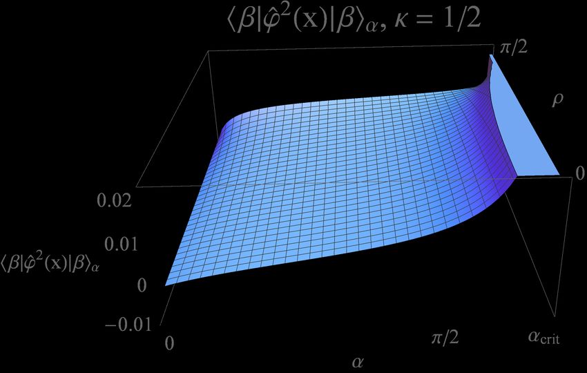
h0|ϕ̂2 |0iα = lim [GEα (x, x0 ) − GES (x, x0 )] , (4.2a)
x0 →x
hβ|ϕ̂2 |βiα = lim 0 0
E
0
G α,β (x, x ) − GE
S (x, x ) , (4.2b)
x →x
where the superscript E refers to quantities constructed on the Euclidean space-time
(4.1). As previously, |0iα denotes a vacuum state with the scalar field satisfying Robin
boundary conditions, while we use the notation |βiα to denote a thermal state at inverse
temperature β, again with Robin boundary conditions applied.
For a thermal state at temperature T , the time coordinate τ is assumed to be
periodic with periodicity 2πβ = 2π/T . The temperature T here is arbitrary, in other
words, there exist thermal states satisfying the Hadamard condition at any temperature.
This is in contrast to the Euclidean version of a black hole space-time, where there is
a natural temperature associated with the black hole horizon and 2πT is the surface
gravity of the black hole. Returning to CAdS, unlike the Lorentzian calculation, the
periodicity in Euclidean “time” forces a discrete integer frequency spectrum independent
of the boundary conditions imposed on the field. Hence the thermal Euclidean Green’s
function assumes the mode-sum representation
∞ ∞
κ X X
GEα,β (x, x0 ) = cos ρ cos ρ 0
e inκ∆τ
(2` + 1)P` (cos γ)gω` (ρ, ρ0 ) (4.3)
8π 2 L2 n=−∞ `=0
where ω = nκ is the quantized frequency, γ is the angular separation of the space-
time points (3.18), gω` (ρ, ρ0 ) is the one-dimensional Green’s function satisfying the
inhomogeneous equation
d 2 d
sin ρ 2 2
− ω sin ρ − `(` + 1) gω` (ρ, ρ0 ) = δ(ρ − ρ0 ), (4.4)
dρ dρQuantum field theory on global anti-de Sitter space with Robin boundary conditions 18
and we have introduced the quantity
κ = 2πT (4.5)
to make the notation a little more compact. For vacuum states, the coordinate τ is
not periodic and the frequency is not quantized. Hence the vacuum Euclidean Green’s
function has the mode-sum representation
Z ∞ ∞
0 1 0
X
E
Gα (x, x ) = 2 2 cos ρ cos ρ dω eiω∆τ (2` + 1)P` (cos γ)gω` (ρ, ρ0 ). (4.6)
8π L ω=−∞ `=0
The one-dimensional Green’s function gω` (ρ, ρ0 ) is constructed from a normalized
product of solutions of the homogeneous version of (4.4),
pω` (ρ< )qω` (ρ> )
gω` (ρ, ρ0 ) = E
, (4.7)
Nω`
where pω` (ρ) is the solution which is regular at the origin ρ = 0, the function qω` (ρ) is
the solution satisfying the boundary conditions at the CAdS boundary ρ = π/2, and
E
Nω` is a normalization constant. We have adopted the notation ρ< ≡ min{ρ, ρ0 } and
ρ> ≡ max{ρ, ρ0 }. The general solution of the homogeneous version of (4.4) can be
expressed in terms of Conical (Mehler) functions as
h i
−`−1/2 −`−1/2
pω` , qω` ∼ (sin ρ)−1/2 C1 Piω−1/2 (cos ρ) + C2 Piω−1/2 (− cos ρ) , (4.8)
where C1 and C2 are arbitrary constants. Imposing regularity at the origin ρ = 0
requires
−`−1/2
pω` (ρ) = (sin ρ)−1/2 Piω−1/2 (cos ρ), (4.9)
the overall constant being irrelevant since it can be absorbed into a redefinition of Nω`
E
.
π
It is at the boundary ρ = 2 where there is freedom to choose boundary conditions.
Taking, without loss of generality,
h i
−1/2 α −`−1/2 −`−1/2
qω` = (sin ρ) Cω` Piω−1/2 (cos ρ) + Piω−1/2 (− cos ρ) , (4.10)
α
where Cω` is a constant, and imposing Robin boundary conditions on qω` analogous to
(2.9),
dqω` (ρ)
qω` (ρ) + tan α = 0, ρ → π/2, (4.11)
dρ
α
fixes the constant Cω` to be
α 2|Γ( iω+`+2
2
)|2 tan α − |Γ( iω+`+1
2
)|2
Cω` = . (4.12)
2|Γ( iω+`+2
2
)|2 tan α + |Γ( iω+`+1
2
)|2
This reduces to Cω`
D
= −1 for Dirichlet boundary conditions whence
h i
−`−1/2 −`−1/2
D
qω` (ρ) = (sin ρ)−1/2 Piω−1/2 (− cos ρ) − Piω−1/2 (cos ρ) , (4.13)Quantum field theory on global anti-de Sitter space with Robin boundary conditions 19
while Cω`
N
= 1 for Neumann boundary conditions and
h i
N −1/2 −`−1/2 −`−1/2
qω` (ρ) = (sin ρ) Piω−1/2 (− cos ρ) + Piω−1/2 (cos ρ) . (4.14)
α
It is useful to reexpress the function qω` for general Robin boundary conditions in terms
of a combination of these two special cases as
α −`−1/2
qω` D
(ρ) = qω` (ρ) cos2 α + qω`
N
(ρ) sin2 α + (Cω`
α
+ cos 2α) (sin ρ)−1/2 Piω−1/2 (cos ρ). (4.15)
We will see below that the benefit of this particular form is that all the divergences
in the Euclidean Green’s function come from the first two terms here; the mode-sum
involving the last term is finite in the coincidence limit.
The final step in the construction of the mode-sum representation of the Euclidean
Green’s function is computing the normalization constant in (4.7). In order for gω` (ρ, ρ0 )
to be a Green’s function, we must have Nω` E
= sin2 ρ W{pω` , qω` } where W denotes the
Wronskian of the solutions. This is straightforwardly calculated to be
E
2
Nω` = . (4.16)
|Γ(` + 1 + iω)|2
Note that this is independent of α.
Putting all of this together, and after some algebra, we obtain the following useful
expressions for the Euclidean Green’s functions for vacuum and thermal states:
GEα (x, x0 ) = GED (x, x0 ) cos2 α + GEN (x, x0 ) sin2 α + GER (x, x0 ) sin 2α, (4.17a)
E 0 E 0 2 E 0 2 E 0
Gα,β (x, x ) = G D,β (x, x ) cos α + G
N,β (x, x ) sin α + GR,β (x, x ) sin 2α, (4.17b)
where GED (x, x0 ), GED,β (x, x0 ) are the Euclidean Green’s functions for Dirichlet boundary
conditions given by
Z ∞ ∞
0 1 cos ρ cos ρ0 iω∆τ
X
E
GD (x, x ) = √ dω e (2` + 1)P` (cos γ)|Γ(` + 1 + iω)|2
16π 2 L2 sin ρ sin ρ0 ω=−∞ `=0
h i
−`−1/2 −`−1/2 −`−1/2
× Piω−1/2 (cos ρ< ) Piω−1/2 (− cos ρ> ) − Piω−1/2 (cos ρ> ) , (4.18a)
∞ ∞
κ cos ρ cos ρ0 X inκ∆τ X
GED,β (x, x0 ) = √ e (2` + 1)P` (cos γ)|Γ(` + 1 + inκ)|2
16π 2 L2 sin ρ sin ρ0 n=−∞ `=0
h i
−`−1/2 −`−1/2 −`−1/2
× Pinκ−1/2 (cos ρ< ) Pinκ−1/2 (− cos ρ> ) − Pinκ−1/2 (cos ρ> ) , (4.18b)
GEN (x, x0 ), GEN,β (x, x0 ) are the Euclidean Green’s function for Neumann boundary
conditions given by
Z ∞ ∞
0 1 cos ρ cos ρ0 iω∆τ
X
E
GN (x, x ) = √ dω e (2` + 1)P` (cos γ)|Γ(` + 1 + iω)|2
16π 2 L2 sin ρ sin ρ0 ω=−∞ `=0
h i
−`−1/2 −`−1/2 −`−1/2
× Piω−1/2 (cos ρ< ) Piω−1/2 (− cos ρ> ) + Piω−1/2 (cos ρ> ) , (4.19a)
∞ ∞
0 κ cos ρ cos ρ0 X inκ∆τ X
G E
N,β (x, x ) = √ e (2` + 1)P` (cos γ)|Γ(` + 1 + inκ)|2
16π 2 L2 sin ρ sin ρ0 n=−∞ `=0
h i
−`−1/2 −`−1/2 −`−1/2
× Pinκ−1/2 (cos ρ< ) Pinκ−1/2 (− cos ρ> ) + Pinκ−1/2 (cos ρ> ) , (4.19b)Quantum field theory on global anti-de Sitter space with Robin boundary conditions 20
and GER (x, x0 ), GER,β (x, x0 ) are two-point functions (not Green’s functions) whose mode-
sum representations are
Z ∞ ∞
0 1 cos ρ cos ρ0 iω∆τ
X
E
GR (x, x ) = 2 2
√ 0
dω e (2` + 1)P` (cos γ)|Γ(` + 1 + iω)|2
16π L sin ρ sin ρ ω=−∞ `=0
" #
iω+`+2 2 iω+`+1 2
2|Γ( 2 )| cos α − |Γ( 2 )| sin α −`−1/2 −`−1/2
× iω+`+2 2 iω+`+1 2
Piω−1/2 (cos ρ)Piω−1/2 (cos ρ0 ),
2|Γ( 2 )| sin α + |Γ( 2 )| cos α
(4.20a)
0 ∞ ∞
κ cos ρ cos ρ X X
GER,β (x, x0 ) = √ einκ∆τ (2` + 1)P` (cos γ)|Γ(` + 1 + inκ)|2
16π 2 L2 sin ρ sin ρ0 n=−∞ `=0
" #
2|Γ( inκ+`+2 )|2 cos α − |Γ( inκ+`+1 )|2 sin α −`−1/2 −`−1/2
× 2 2
Pinκ−1/2 (cos ρ)Pinκ−1/2 (cos ρ0 ).
2|Γ( inκ+`+2
2
)|2 sin α + |Γ( inκ+`+1
2
)|2 cos α
(4.20b)
The two-point functions GER (x, x0 ), GER,β (x, x0 ) can be interpreted as the regular
contributions to the vacuum and thermal Green’s function as a result of considering
general Robin boundary conditions. These contributions are evidently vanishing for
Dirichlet and Neumann boundary conditions by merit of the sin 2α factor in (4.17). In
this sense, we can think of the subscript R as representing either ‘Robin’ or ‘Regular’.
To see that the mode-sums (4.20) are indeed regular for any Green’s functions (4.17)
satisfying the Hadamard condition, we note that both the Dirichlet (4.18) and Neumann
(4.19) Green’s functions are known to satisfy the Hadamard condition. Hence the
singularities in the first two terms of (4.17) are given by cos2 α GES + sin2 α GES = GES
where GES is the Hadamard parametrix for the Euclidean wave equation. Hence all
the singularities for a propagator satisfying the Hadamard condition are contained in
the first two terms of (4.17), which implies that both GER and GER,β are regular in the
coincidence limit. This is in accordance with the fact that GER and GER,β are solutions of
the homogeneous scalar field equation.
The contrapositive of the above argument is that if either GER or GER,β is not regular
in the coincidence limit, then the corresponding Green’s function GEα or GEα,β is not
Hadamard. In this case the corresponding quantum state is not a Hadamard state and
should not be considered as physically meaningful. It is clear from the explicit mode-
sum representation (4.20) that GER or GER,β diverges if there exists a value of the constant
α and mode numbers (ω, `) for which
|Γ( iω+`+1
2
)|2
2 tan α = − , (4.21)
|Γ( iω+`+2
2
)|2
which is precisely the condition (2.12) for unstable modes. In other words, the quantum
state for the Robin boundary condition (2.9) is a Hadamard state only for those values
of α for which the classical scalar field has no unstable modes.Quantum field theory on global anti-de Sitter space with Robin boundary conditions 21
4.2. Equivalence of the Euclidean and Lorentzian Green’s functions for Dirichlet and
Neumann boundary conditions
One advantage of the representation (4.17) is that we will be able to use known
expressions for the Dirichlet and Neumann propagators to simplify the Green’s function
for general Robin boundary conditions. The thermal propagator on CAdS for Dirichlet
and Neumann boundary conditions can be obtained as an infinite image sum of the
corresponding zero-temperature Green’s function on the Lorentzian space-time [2]. It
is not at all obvious how to connect that expression to the mode-sum representations
(4.18, 4.19) derived here using Euclidean methods. In this section we therefore present
the details of this calculation, proving that, for Dirichlet and Neumann boundary
conditions, the thermal Euclidean Green’s functions (4.18b, 4.19b) are equivalent to
the anticommutators for the field at finite temperature on the Lorentzian space-time
under the mapping ∆t → i∆τ .
We will show in detail how to obtain the thermal anticommutator derived in [2]
for the Dirichlet case from our mode-sum (4.18b). The calculation for the Neumann
case is almost identical. We start with the generalized addition theorem for Gegenbauer
functions Cλξ [64]
Cλξ (x x0 − z(1 − x2 )1/2 (1 − x02 )1/2 )
∞
Γ(2ξ − 1) X (−1)` 4` Γ(λ − ` + 1)Γ(` + ξ)2
=
|Γ(ξ)|2 `=0 Γ(λ + 2ξ + `)
ξ+` ξ+` ξ−1/2
× (2` + 2ξ − 1)(1 − x2 )`/2 (1 − x02 )`/2 Cλ−` (x< )Cλ−` (x> )C` (z), (4.22)
where x< ≡ min{x, x0 } and x> ≡ max{x, x0 }. This is valid for any complex λ for which
both sides of the equality are well-defined. Now taking ξ = 1, λ = inκ − 1 and using
the relationship between Legendre and Gegenbauer functions gives
∞
1 X −`−1/2 −`−1/2
√ 0
(2` + 1)P` (cos γ) |Γ(` + 1 + inκ)|2 Pinκ−1/2 (cos ρ< )Pinκ−1/2 (− cos ρ> )
sin ρ sin ρ `=0
−1/2
√ nκ Pinκ−1/2 (cos Ψ)
= − 2π √ , (4.23)
sinh πnκ sin Ψ
where
Ψ = cos−1 (− cos ρ cos ρ0 − cos γ sin ρ sin ρ0 ) . (4.24)
The particular conical functions appearing on the right-hand-side of (4.23) reduce to
−1/2
Pλ+1/2 (cos z)
r
2 1 sin(λ + 1)z
√ = . (4.25)
sin z π (λ + 1) sin z
We thus arrive at the following summation formula
∞
1 X −`−1/2 −`−1/2
√ 0
(2` + 1)P` (cos γ) |Γ(` + 1 + inκ)|2 Pinκ−1/2 (cos ρ< )Pinκ−1/2 (− cos ρ> )
sin ρ sin ρ `=0
2 sinh nκΨ
= . (4.26)
sinh πnκ sin ΨYou can also read