Temporal Cluster Matching for Change Detection of Structures from Satellite Imagery - Daniel E. Ho
←
→
Page content transcription
If your browser does not render page correctly, please read the page content below
Temporal Cluster Matching for Change Detection of Structures
                                                               from Satellite Imagery
                                             Caleb Robinson1 , Anthony Ortiz1 , Juan M. Lavista Ferres1 , Brandon Anderson2 , and
                                                                                 Daniel E. Ho2
                                                                        1
arXiv:2103.09787v1 [cs.CV] 17 Mar 2021

                                                                            Microsoft AI for Good Research Lab
                                                                                    2
                                                                                      Stanford RegLab

                                                                                          Abstract
                                                   We propose a general model, Temporal Cluster Matching (TCM), for detecting building
                                               changes in time series of remotely sensed imagery when footprint labels are only available for a
                                               single point in time. The intuition behind the model is that the relationship between spectral
                                               values inside and outside of building’s footprint will change when a building is constructed (or
                                               demolished). For instance, in rural settings, the pre-construction area may look similar to the
                                               surrounding environment until the building is constructed. Similarly, in urban settings, the pre-
                                               construction areas will look different from the surrounding environment until construction. We
                                               further propose a heuristic method for selecting the parameters of our model which allows it to
                                               be applied in novel settings without requiring data labeling efforts (to fit the parameters). We
                                               apply our model over a dataset of poultry barns from 2016/2017 high-resolution aerial imagery
                                               in the Delmarva Peninsula and a dataset of solar farms from a 2020 mosaic of Sentinel 2 imagery
                                               in India. Our results show that our model performs as well when fit using the proposed heuristic
                                               as it does when fit with labeled data, and further, that supervised versions of our model perform
                                               the best among all the baselines we test against. Finally, we show that our proposed approach
                                               can act as an effective data augmentation strategy – it enables researchers to augment existing
                                               structure footprint labels along the time dimension and thus use imagery from multiple points
                                               in time to train deep learning models. We show that this improves the spatial generalization of
                                               such models when evaluated on the same change detection task.

                                         1    Introduction
                                         Catalogs of high-resolution remotely sensed imagery have become increasingly available to the sci-
                                         entific community. The availability of such imagery has revolutionized scientific fields and society
                                         at large. For example, 1m resolution aerial imagery from the US Department of Agriculture (NAIP
                                         imagery) has been released on a 2-year rolling basis over the entire US for over a decade and the com-
                                         mercial satellite imagery provider, Planet, recently started to release 5m satellite imagery covering
                                         the whole tropical forest region of the world on a monthly basis. One estimate is that the opening
                                         of Landsat imagery in 2008 led to the creation of $3.45B in economic value in 2017 alone (1). The
                                         accumulation of such data facilitates an entirely new branch of longitudinal studies – analyzing the
                                         Earth and how it has changed over time.
                                             As the climate, technology, and human population change on an ever more rapid timescale, such
                                         longitudinal studies become particularly vital to understanding the past, present, and future of the

                                                                                              1
environment. Despite the usefulness of time series data, such research quickly faces two practical
challenges. First, the large labeled datasets that have fueled advances in computer vision are much
more limited in the satellite imagery context (2; 3; 4). Second, efforts in creating labeled data
from remotely sensed imagery are typically focused on a single point in time (2; 5; 6; 3). Project
requirements may only call for a single layer of labels, or budget constraints may limit the number
of labels that can be generated. This has the effect of creating labeled datasets that are “frozen” in
time. Expanding such “frozen” datasets to multiple points in time in independent follow-up work
can be difficult as the same image-preprocessing and labeling methodology steps used in the original
work need to be precisely reproduced in order to generate comparable data.
Going beyond “frozen” datasets would enable a wide range of temporal inferences from satellite
imagery, with significant social, economic, and policy implications. Previous studies include the
detection of urban expansion (7), zoning violations (8), habitat modification (9), compliance with
agricultural subsidies (10), construction on wetlands (11), and damage assessments from natural
disasters (12; 13; 14).
Algorithmic approaches for expanding “frozen” datasets can thus be useful in facilitating ecologi-
cal and policy-based analysis. In this work we propose a model, Temporal Cluster Matching (TCM),
for determining when structures were previously constructed given a labeled dataset of structure
footprints generated from imagery captured at a particular point in time. This model, importantly,
does not rely on the differences in spectral values between layers of remotely sensed imagery as there
can be considerable variance in these values depending on imaging conditions, the type of sensor
used, etc. Instead, it compares a representation of the spectral values inside a building footprint
to a representation of the spectral values in the surrounding area for each point in the time series.
Whenever the distribution of spectral values within the footprint becomes dissimilar to that of its
surroundings then the footprint is likely to have been developed. We further propose a method for
fitting the parameters of this model which does not rely on additional labeled footprint data over
time and show that this “semi-supervised TCM” performs comparably to supervised methods.
Specifically, we demonstrate the performance of this algorithm in two distinct settings:
1. Poultry barns from concentrated animal feeding operations (CAFOs) in the United States,
using high-resolution aerial imagery from the National Agricultural Imagery Program (NAIP),
and
2. Solar farm footprints in the Indian state of Karnataka, using Sentinel 2 annual mosaics.
Both settings are of significant environmental importance and are ripe for longitudinal study.
First, CAFOs can have profound effects on water quality and human health in their proximity
(15). Nitrates and other potentially harmful chemicals can, for example, make their way into
the groundwater, spreading to adjacent wells and bodies of water over timescales that range into
decades. Usage of antibiotics for growth promotion can lead to resistant bacterial infections in
nearby populations (16). Effective regulation in either scenario requires differentiation of these
contaminant sources, which, in turn, depends on accurate historical labels and spatio-temporal
modeling.
Second, understanding the growth of solar systems is increasingly important in the transition
toward clean energy. India is an important example of this, as it has set ambitious goals of generating
450 GW of renewable energy by 2030 with 175 GW deployment by 2022 (17). Achieving this goal
will require an expansion of solar farm installations throughout the country and policy makers will
be able to determine better the effects of country-wide efforts with solar farm change data that can
2be updated year-over-year in a consistent manner. Understanding such solar expansion may also
enable more targeted investments for solar potential (18).
To summarize, our contributions include:
• A new model, Temporal Cluster Matching, for detecting when structures are developed in a
time-series of remotely sensed imagery, as well as a heuristic method for fitting the parameters
of the model. Combined, this results in a proposed approach that only relies on labeled
building footprints for a single point in time.
• A series of baseline methods, both supervised and semi-supervised, to evaluate our proposed
approach against.
• Experiments comparing our model to the baseline models in two datasets: poultry barn
footprints with aerial imagery, and solar farm footprints with satellite imagery.
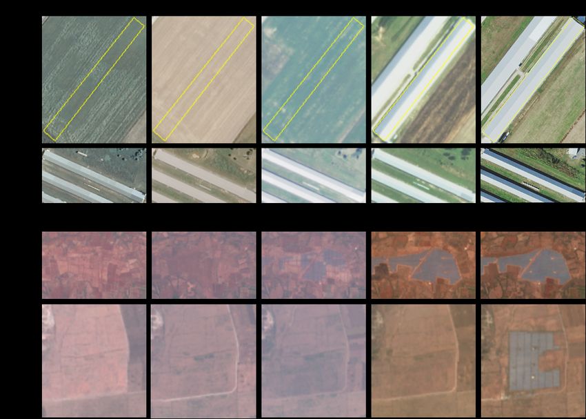
Figure 1: (A and B) Examples of two poultry barn footprints over 5 years of NAIP imagery.
We observe inter-year variability of NAIP imagery and the change in the relation of color/texture
between the footprint and neighborhood when a footprint is “developed”. (C and D) Examples of
two solar farm footprints over 5 years of Sentinel 2 imagery. Note, in A we outline the building
footprint location in yellow through the entire series of imagery, but omit this outline in remaining
rows.
32 Related Work
Our work pertains to several different literatures. First, much work has focused on methods for
detection of building footprints (19; 20). For instance, (20) uses Mask R-CNN to train a model to
detect buildings while (21) uses a semantic segmentation model (U-Net (22)) to segment buildings
in imagery. While deep learning approaches have made rapid advances, they have largely been
focused on static inferences. Moving to a different domain (spatially or temporally) can hence prove
challenging. Zhang et al., for instance, note that one of the challenges has been the inaccuracy of
human labeling of structures (23).
Second, other research has focused on detecting changes in satellite imagery. Historically, the
remote sensing literature has started from pixel-wise changepoint detection, which is known to be
sensitive to changes in image characteristics (e.g., illumination, seasonality). (24) propose object-
based temporal adjustments to improve intertemporal consistency of imagery. Other advances have
utilized machine learning for building changepoint detection. (25) uses decision trees to classify
whether a building change occurred. (26) uses Support Vector Machines to provide estimates for
which buildings have changed. Most recently, advances in deep learning have driven forward end-
to-end pipelines in building change detection. (27), for instance, uses a Generative Adversarial
Network (GAN) to overcome the limitations of pixel-level inferences.
Third, numerous research teams have provided benchmark datasets for single points in time
(2; 5; 6; 3). Few datasets provide longitudinal information about the same location over time, so a
typical research approach has been to train a model on labeled imagery from one period. (28), for
instance, assess the growth of intensive livestock farms in North Carolina, but do so using a model
trained on images of such facilities for a single period of time. Domain adaptation to other years of
imagery can pose challenges due to differences in image illumination, seasonality, and angle (29).
Our approach contributes to this body of work by providing a semi-supervised approach that
easily enables researchers to expand a dataset beyond a single time period, hence enabling domain
adaptation by efficient sampling of images across time. The approach we propose can be seen as a
lightweight, data-driven method to expand “frozen” imagery longitudinally, enabling researchers to
address a rich set of dynamic questions.
3 Methods
3.1 Problem statement
Formally, we would like to find when a structure was developed (or, more
1generally, changed) given a
time series of remotely sensed imagery of it and the surrounding area, X , . . . , X and its footprint,
t
P , at time t. We represent this footprint as a mask, Yt . Here, the ith image in the time series
Xi ∈ Zw×h×c is a georeferenced image with width, w, height, h, and number of spectral bands, c.
Similarly, Yt ∈ {0, 1}w×h is a georeferenced binary mask with the same dimensions that contains a
1 in every spatial location that the given structure covers at time t and a 0 elsewhere. We want to
estimate the point in time that the structure was created, i.e. find l ∈ [1, t], where Xl contains the
structure, for the smallest such l. Note that we assume the structure to exist at t.
3.2 Temporal Cluster Matching
Our proposed model, Temporal Cluster Matching, relies on the assumption that when a structure
is built its footprint will have a different set of colors and textures than its immediate surroundings
4Algorithm 1: Temporal Cluster Matching
Input: Time series of remotely sensed imagery, P , k, r, and θ
1 1 l, thet first point in time that the footprint described by P was developed
Output:
1 X , X , . . . , X ← crop the imagery according to the buffered extent of P by a radius r
2 Y ← rasterize P in the same buffered extent
t
3 for l ← 1 to t do
4 C ← cluster indices from a k-means clustering of Xl into k clusters
5 Dfootprint ← distribution of cluster indices C[Yt = 1]
6 Dneighborhood ← distribution of cluster indices C[Yt = 0]
7 d ← DKL (Dfootprint || Dneighborhood )
8 if d > θ then
9 return l
10 end
11 end
12 return t
compared to when the structure was not built. For example, an undeveloped piece of land in a rural
setting will likely contain some sort of vegetation, and that vegetation will probably look similar
(in color/texture) to some of its surroundings. When a structure is built on this land, then it will
likely look dissimilar to its surroundings (unless e.g. its entire surroundings are also developed at
the same time). The same intuition holds in urban environments – an undeveloped piece of land
will look dissimilar to its surroundings, however, when it is developed, it will look similar.
We assume that we are given a footprint, P , that outlines a structure that has been labeled as
developed at time t. Now, we formally define the neighborhood of this footprint. This neighbor-
hood should be larger than the extent of the footprint in order to observe a representative set of
colors/textures, so we let r be a radius that serves as a buffer to the building footprint
polygon.
We then create Yt by rasterizing the polygon within this buffered extent and create X0 , . . . , Xt
by cropping the same buffered extent from each layer of remotely sensed imagery.
Next, we define a method for comparing the set of colors/textures within the footprint to those
in the surrounding neighborhood. Given a single layer of remotely sensed image from the time se-
ries, X, we run k-means to partition the pixels into k clusters. Each pixel can be represented by a
set of features that encodes color and texture at its location, for example: the spectral values at the
pixel’s location, a texture descriptor (such as a local binary pattern) at the location, the spectral
values in a window around the location, or some combination of the previous representations. Re-
gardless, the cluster model will assign a cluster index to each pixel in X which we call C. We then
represent an area by the discrete distribution of cluster indices observed in that area. Specifically,
we let Dfootprint be the distribution of cluster indices from C[Yt = 1] and Dneighborhood be the distri-
bution of cluster indices from C[Yt = 0]1 . Now, we can compare the set of colors/textures within a
footprint to those in its surrounding neighborhood by calculating the KL-divergence between the two
1
We use the notation C[Yt = 1] to mean all the cluster indices of pixels where Yt = 1. We build the discrete
distribution by counting the number of pixels assigned to each cluster and normalizing the vector of counts by its
sum.
5Figure 2: We show the distribution of KL divergence values generated by our proposed approach
for (1) poultry barn footprints in aerial imagery where there is guaranteed to be a structure and (2)
randomly generated footprints over similar aerial imagery. We observe that (1) is unimodal with a
large mean value, as the color distributions of footprints that contain buildings are dissimilar to the
color distribution of their surroundings and (2) is unimodal with a small mean value, as random
patches are highly likely to have a color distribution that is similar to their neighborhood. Our
proposed heuristic method looks to find hyperparameters for the model that minimize the overlap
in these two distributions such that a simple threshold can identify changes in building footprints.
distributions of cluster indices, d = DKL (Dfootprint || Dneighborhood ). Larger KL-divergence values
mean that the color/texture of a footprint is dissimilar to that of its surrounding neighborhood and
that it is likely to be developed. We perform this comparison method for each image in the time
series to create a list of KL-divergence values [d1 , . . . , dt ]
Finally, we let θ be a threshold value to determine the smallest KL-divergence value that we will
consider to indicate a “developed” footprint. More specifically, our model will estimate l as the time
that a footprint is first developed for the first l where dl > θ. This parameter can be found by
experimentation using labeled data, or with the heuristic method we describe in Section 3.3. See
Algorithm 1 for an overview of this proposed approach.
We explore using more complex decision models, then the single threshold described above, in
Section 3.4, however note that these require labeled data to fit.
3.3 A heuristic for semi-supervised Temporal Cluster Matching
In application scenarios we would like to use our model, given a dataset of (a) known structure
footprints at time t and (b) a time series of remotely sensed imagery over a certain study area, to
find when each structure was constructed. Here we propose a method for determining reasonable
parameter values for the number of clusters, k, buffer radius, r, and decision threshold, θ, without
assuming that we have prior labeled data on construction dates.
This heuristic compares the distribution of KL-divergence values calculated by our algorithm
for given hyperparameters, k and r, over all footprints at time t (when we assume that structures
6exist) to the distribution of KL-divergence values over a set of randomly generated polygons over the
study area. The intuition is that the relationship between random polygons and their neighborhoods
is similar to the relationship between undeveloped structure footprints and their neighborhoods. In
other words, this distribution of KL divergence values between color distributions from random
polygons and their surroundings will represent what we would expect to observe by chance – i.e.
not the relationship between the colors in a building footprint and its surroundings. We want to
find parameter settings for our algorithm that minimize the overlap between these two distributions
because it will make it easier to identify change (see Figure 2 for an illustration of this for poultry
barn footprints). Formally, we let p be the distribution of KL-divergence values over footprints at t
and q be the distribution of KL-divergence values over random polygons sampled from the study area
(over all points in time). These are discrete distributions (e.g after binning KL divergencep values)
and we can measure the overlap with the Bhattacharyya coefficient, BC(p, q) = x∈X p(x)q(x).
P
Choosing k and r thus becomes a search mink,r BC(p, q).
Finally, after choosing k and r, we can simply choose θ as a value representing the 98th percentile
(or similar) of the resulting distribution of random polygons, q. Practically, this value simply needs
to separate p and q and visualization of these two distributions should suggest appropriate values.
We test this heuristic in Section 5.1 by comparing change detection performance from fitting
our proposed model with this heuristic versus with labeled data.
3.4 Baseline approaches
Here we propose a series of baselines and variants of our model to compare against. We refer to
our proposed model / heuristic for fitting the model as “Semi-supervised TCM” as it only depends
on labeled building footprints from a single point in time. This is specifically in contrast to variant
approaches like “Supervised TCM” (see below) that use labeled building footprints over time to fit
the model parameters.
Supervised TCM Here, we fit the parameter θ in our proposed model using labeled data instead
of our proposed heuristic. We can do this by searching over values of θ and measuring per-
formance on the labeled data. In this case, k and r are model hyperparameters that can be
searched over using validation data.
Supervised TCM with LR We use the series of KL-divergence values computed by TCM as a
feature representation in a logistic regression (LR) model that directly predicts which point
in time a structure is first observed. This is a supervised method as it requires a sample of
labeled footprint data over time to fit.
Average-color with threshold This baseline uses the same structure as TCM with two changes:
instead of clustering colors we compute average colors representations (over space for each spec-
tral band) and instead of computing KL-divergence between distributions of cluster indices
we compute the Euclidean distance between the average colors representations. Specifically,
we compute the average color in a footprint and the average color of its neighborhood, then
take the Euclidean distance between them and treat this distance in the same way we have
previously treated the KL-divergence values. This has the effect of removing k as a hyperpa-
rameter, however the rest of the algorithm stays the same. Similar to the KL with threshold
method we fit θ using labeled data.
7Average-color with LR This method is identical to Supervised TCM with LR, but using the
technique from Average-color with threshold to compute Euclidean distances between average
color representations.
Color-over-time In this baseline we compute features from a time series of imagery by averaging
the colors (over space for each spectral band) in the given footprint at each point in time, then
taking the Euclidean distance between these average representations in subsequent pairs of
imagery. For example, a time series of 5 images would result in an overall feature representation
of 4 distances: the distance between the average colors at time 1 and average colors at time
2, the distance between the average colors at time 2 and the average colors at time 3, etc. We
use this overall representation in a logistic regression model that predicts which point in time
the structure is first observed.
CNN-over-time In this baseline we use the given structure footprints and satellite imagery at time
t to train a U-Net based semantic segmentation model to predict whether or not each pixel in
an image contains a developed structure. We then use this trained model to score the imagery
from each point and time and determine the first layer in which a building is constructed. For
simplicity, if the network predicts that over 50% of a footprint is constructed, then we count
it as constructed.
Mode predictions This baseline is simply predicting the most frequent time point that we first
observe constructed buildings based on the labels in the dataset of interest.
4 Datasets
4.1 Poultry barn dataset
We use the Soroka and Duren dataset of 6,013 labeled poultry barn polygons, Poultry barn,
created from NAIP 2016/2017 imagery over the Delmarva Peninsula (containing portions of Virginia,
Maryland, and Delaware) (30). As NAIP is collected independently by each state at least once every
three years on a rolling basis, the availability and quality of the imagery varies between states. For
instance, the NAIP imagery from 2011 in Delaware and Maryland was collected on different days,
at different times of day, etc. See Figure 1 for example images of the NAIP imagery over time
overlayed with the barn footprints. Additionally, we have manually labeled the earliest year (out
of the years shown in Table 1) that a poultry barn can be seen for a random subset of 1,000 of the
poultry barn footprints.
State Years of NAIP data
Delaware 2011, 2013, 2015, 2017, 2018
Maryland 2011, 2013, 2015, 2017, 2018
Virginia 2011, 2012, 2014, 2016, 2018
Table 1: NAIP data availability over states covering the Delmarva Peninsula.
84.2 Solar farm dataset
We also use a solar farm dataset, Solar farm, containing polygons delineating solar installations
in the Indian state of Karnataka for the year 2020. The dataset includes 935 individual polygons
covering a total area or 25.7 km2 . The polygons were created by manually filtering the results of a
model run on an annual median composite of Sentinel 2 multispectral surface reflectance imagery.
We collect additional median composites of Sentinel 2 imagery for 2016 through 20192 to use for
change detection. See Figure 1 for examples of the imagery overlayed with the solar farm footprints.
For each of the 935 footprints we have manually labeled the earliest year (between 2016 and 2020)
that a solar farm can be seen in the imagery.
Method Semi-Supervised ACC MAE
Semi-supervised TCM X 0.94 0.15
CNN over time X 0.37 1.36
Supervised TCM with LR 0.96 +/- 0.01 0.12 +/- 0.03
Poultry barn
Average-color with LR 0.95 +/- 0.01 0.15 +/- 0.05
Supervised TCM 0.93 +/- 0.01 0.17 +/- 0.04
Average-color with threshold 0.91 +/- 0.02 0.24 +/- 0.06
Color-over-time 0.90 +/- 0.02 0.41 +/- 0.08
Mode predictions 0.84 0.80
Semi-supervised TCM X 0.71 0.49
CNN over time X 0.64 0.68
Supervised TCM with LR 0.78 +/- 0.03 0.29 +/- 0.05
Solar farm
Average-color with LR 0.65 +/- 0.03 0.49 +/- 0.05
Supervised TCM 0.70 +/- 0.04 0.51 +/- 0.08
Average-color with threshold 0.50 +/- 0.04 0.93 +/- 0.08
Color-over-time 0.79 +/- 0.01 0.29 +/- 0.02
Mode predictions 0.42 0.81
Table 2: Comparison of our proposed semi-supervised model (“Semi-supervised TCM”) to other
baseline methods for detecting change in structures over time series of imagery. Note that the semi-
supervised methods only have access to building footprint labels at time t, while the other methods
are “supervised” and additionally have access to labels on when buildings were constructed over time.
We observe that our semi-supervised approach achieves identical performance to a supervised variant
where the model parameters are learned. We further observe the proposed approach outperforms
supervised baseline methods for detecting change. Reported values are shown as averages (+/-) a
standard deviation over 50 random train/test splits where appropriate. Single values are reported
for the semi-supervised methods as they are evaluated on the entire labeled data set.
2
The data from 2016, 2017 and 2018 are composites of the Sentinel 2 top of atmosphere products (Level 1C),
while the 2019 and 2020 data are additionally corrected for surface reflectance (Level 2A). All data was processed
with Google Earth Engine using the COPERNICUS/S2 and COPERNICUS/S2_SR collections respectively.
95 Experiments and results
We experiment with different configurations of our algorithm on the Poultry barn and Solar
farm datasets. In all experiments we measure the accuracy (ACC) – the percentage of labeled
footprints for which we correctly identify the first “developed” year and mean absolute error (MAE)
– the average of absolute differences between the predicted year and labeled year.
5.1 Semi-supervised TCM
We first test how parameters chosen with the proposed heuristic correlate with performance of the
model. The benefit of the heuristic method is that it does not require labeled temporal data to fit the
model, but we need to show that the parameters it selects actually result in good performance. Here,
we search over buffer sizes in {100, 200, 400} meters and {0.016, 0.024} degrees for the Poultry
barn and Solar farm datasets, respectively, and number of clusters in {16, 32, 64} for both
datasets. For each configuration combination we create p and q as described in Section 3.3, compute
the Bhattacharyya coefficient, estimate θ, then evaluate the predicted change years on the labeled
data. We find that the Bhattacharyya coefficient is correlated with the result; there is -0.77 rank
order correlation between the coefficient and accuracy (p=0.01) in Poultry barn and a -0.94
rank order correlation (p=0.004) in Solar farm. In both datasets, the smallest Bhattacharyya
coefficient was paired with the best performing algorithm configuration.
Second, we compare the performance of the model with heuristic estimated parameters to that
with learned parameters. To learn the parameters for our proposed model, “Supervised TCM”, we
randomly partition the labeled time series data into 80/20 train/test splits. We find the values of
k, r, and θ (with a grid search over the same space for k and r as mentioned above) using the
training split, then evaluate this model on the test split. We repeat this process for 50 random
partitions and report the average and standard deviation metrics for the best combination Table 2.
We observe that the heuristic method produces results that are equivalent to those of the learned
model. In Poultry barn our proposed method achieves a 94% accuracy with a mean absolute
error of 0.15 years which suggests it will be effective for driving longitudinal studies of the growth
of poultry CAFOs.
Finally, we observe that our method significantly outperforms the other semi-supervised baseline,
CNN over time. In both Poultry barn and Solar farm we observe considerable covariate shift.
For example, in the Poultry barn dataset there is a large shift in input distribution over time due
to the fact that the aerial imagery is collected at different days of the year, at different times of day,
etc. The deep learning model is trained solely on imagery from the last point in each time series
where we can confirm that there exists buildings in each footprint, however is unable to reliably
generalize over time. We did not experiment with domain adaptation techniques to attempt to fix
this, however we explore the use of our proposed method in this capacity in Section 6. We note
that our proposed model is unaffected by shifts in the input distributions year-over-year as it never
compares imagery from different years.
5.2 Supervised models
In the previous section we showed that we can estimate the parameters of our model without labeled
time series data. Not requiring additional labeling is a major benefit of the TCM approach. In this
section we explore the performance of our proposed approach against supervised baseline approaches,
using labels generated going back in time. We find that logistic regression models are effective at
10predicting the building construction date from the series of KL divergence values produced by our
propose approach (KL with LR). In both datasets this method is overall the top performing method
with 96% accuracy in the Poultry barn dataset and 78% accuracy in the Solar farm dataset.
In the Solar farm dataset the Color-over-time baseline has tied for top performance (within a
standard deviation), but the same features are not as effective in the Poultry barn dataset where
the color shifts are more dramatic year-over-year. Even so, the performance of the color-over-time
baseline was much better than we originally hypothesized and should be compared to in future work
regardless of perceived covariate shifts.
We also observe that our proposed method (that computes clustered representations) dominates
the family of average-color baselines. This, along with the fact that we observe that more clusters in
the k-means model usually results in better performance, suggests that the clustered representation
is an important component of our approach. We hypothesize that more rich feature representations
will prove even more effective as both the colors and textures of a footprint will change when it
becomes developed. This is a trivial addition to the existing model and we hope to test it in future
studies.
Finally, we observe that our heuristic method performs very well overall. In both datasets there
are only two supervised methods that achieve stronger result.
6 Temporal Cluster Matching as a data augmentation strategy
In Table 2 we show that training semantic segmentation models on structure footprint masks at a
time t does not result in a model that can generalize well over time (and thus cannot detect change).
Previously (in Section 5.1) we hypothesized that this is due to the covariate shift in the time series
imagery in the two datasets that we test on – the Poultry barn dataset uses NAIP aerial imagery
that is collected at different times of day and different days of the year on a rolling three year basis
and the Solar farm dataset uses Sentinel 2 mosaics created from TOA corrected imagery in 2016
through 2018 and surface reflectance corrected imagery in 2019 and 2020, thus a model trained with
data from a single layer in both of these cases is unlikely to perform well in other layers.
Here we test this hypothesis by using our proposed method to augment the data used to train the
CNN over time method for the Poultry barn dataset. Specifically, we run Semi-supervised TCM
over the Poultry barn dataset to create predictions as to when each footprint was constructed.
We then use these estimates to create an expanded training set that contains pairs of imagery over
all time points with footprint masks that are predicted to have a building. For example, if our model
believes that there was a building in a given footprint at 2011 in the NAIP imagery, then we can
train the segmentation model with (NAIP 2011, footprint), (NAIP 2013, footprint), etc. We find
that this increases the performance of the model on the change detection task in all cases that we
tested. For example, we apply this augmentation step to the same model configuration used in the
results from Table 2 and achieve a 56% accuracy and 0.97 MAE (a 19% improvement in ACC and
0.39 improvement in MAE). These results are not competitive with the other methods we test in
the change detection task. This likely stems from the fact that the segmentation model, in contrast
to the other methods, is not specialized to change detection. On the other hand, the segmentation
model can be run over new imagery to find novel instances of poultry barns (e.g., barns destroyed
prior to the date of original data labeling), and is thus necessary to improve the performance of
such models for more general applications.
While a more rigorous evaluation of how to improve the deep learning segmentation baseline
is outside the scope of this paper, we hypothesize that more data augmentation strategies (e.g.
11RandAugment (31) and AugMix (32)), unsupervised domain adaptation methods (33), and a hy-
perparmeter search over dimensions such as class balancing strategies, temporal balancing strategies,
learning rates, architecture, etc. would all improve performance. These types of experimentation
will be critical for any future work that attempts to create general purpose models for detecting
concentrated animal feeding operations or solar farms at scale. That said, one of the main benefits
of our proposed TCM is that it provides a lightweight approach to detect construction.
7 Conclusion and future work
We have proposed Temporal Cluster Matching (TCM) for detecting change in building footprints
from time series of remotely sensed imagery. This model is based on the intuition that the rela-
tionship between the distribution of colors inside and outside of a building footprint will change
upon construction. We further propose a heuristic based method for fitting the parameters of our
model and show that this approach effectively detects poultry barn and solar farm construction.
TCM does not depend on having labels over time, yet it can outperform similar models that have
such labels available. Further, we show that the feature representation from TCM – a sequence
of KL-divergence values between the distribution of color clusters inside and outside of a building
footprint – can be used in supervised models to improve change detection performance. Finally, we
show how TCM can be used as a data augmentation technique for training deep learning models to
detect building footprints from remotely sensed imagery.
This work motivates several future directions. First, the per-pixel representation of TCM will
affect detectable changes. We used simple color representations, but more elaborate representations
could be promising (e.g. texture descriptors or higher dimensional image embeddings). Second,
future work should explore other applications of TCM. Here we experimented with imagery where
the size of the footprints were relatively large compared to the spatial resolution of the imagery.
However, our model may not perform as well when the footprint is relatively smaller. For example,
we briefly experimented with detecting changes using general building footprints in the US and
NAIP imagery and found that the relationship between the color distributions of small residential
buildings and their surroundings was very noisy, but did not attempt to investigate further. The top
performing methods from the recent SpaceNet7 challenge run their building detection algorithms
on upsampled imagery and a similar strategy may be useful with TCM. Finally, we hypothesize
that TCM would work with time series of imagery from multiple remote sensing sensor modalities.
A benefit of our model is that it does not consider inter-year differences and thus is not affected
by shifts in the color distributions of the imagery, but our experimental results do not explore the
extent in which this is a useful property. Practically, there may be problems (such as shifts in
geolocation accuracy) when applying TCM over stacks of imagery from different sources.
In summary, we hope TCM approach illustrated here will enable researchers to overcome the
“frozen” labels of many emerging earth imagery datasets. Our lightweight approach to augment
labels temporally should foster richer exploration of time series of satellite imagery and help us to
understand the earth as it was, is, and will be.
Acknowledgements
We thank Microsoft Azure for support in cloud computing, and Schmidt Futures, Stanford Impact
Labs, and the GRACE Communications Foundation for research support.
12References
[1] C. L. Straub, S. R. Koontz, and J. B. Loomis, “Economic valuation of landsat imagery,” tech. rep., U.S.
Geological Survey, Reston, VA, 2019. Report.
[2] A. V. Etten, D. Lindenbaum, and T. M. Bacastow, “Spacenet: A remote sensing dataset and challenge
series,” CoRR, vol. abs/1807.01232, 2018.
[3] R. Roscher, M. Volpi, C. Mallet, L. Drees, and J. D. Wegner, “Semcity toulouse: A benchmark for
building instance segmentation in satellite images,” ISPRS Annals of Photogrammetry, Remote Sensing
and Spatial Information Sciences, vol. 5, pp. 109–116, 2020.
[4] I. Demir, K. Koperski, D. Lindenbaum, G. Pang, J. Huang, S. Basu, F. Hughes, D. Tuia, and R. Raskar,
“Deepglobe 2018: A challenge to parse the earth through satellite images,” in Proceedings of the IEEE
Conference on Computer Vision and Pattern Recognition Workshops, pp. 172–181, 2018.
[5] N. Weir, D. Lindenbaum, A. Bastidas, A. V. Etten, S. McPherson, J. Shermeyer, V. Kumar, and
H. Tang, “Spacenet mvoi: a multi-view overhead imagery dataset,” in Proceedings of the IEEE/CVF
International Conference on Computer Vision, pp. 992–1001, 2019.
[6] D. Noever and S. E. M. Noever, “Overhead mnist: A benchmark satellite dataset,” arXiv preprint
arXiv:2102.04266, 2021.
[7] L. Wang, C. Li, Q. Ying, X. Cheng, X. Wang, X. Li, L. Hu, L. Liang, L. Yu, H. Huang, et al., “China’s
urban expansion from 1990 to 2010 determined with satellite remote sensing,” Chinese Science Bulletin,
vol. 57, no. 22, pp. 2802–2812, 2012.
[8] R. Purdy, “Using earth observation technologies for better regulatory compliance and enforcement of
environmental laws,” Journal of Environmental Law, vol. 22, no. 1, pp. 59–87, 2010.
[9] M. J. Evans and J. W. Malcom, “Automated change detection methods for satellite data that can
improve conservation implementation,” bioRxiv, p. 611459, 2020.
[10] A. Moltzau, “Estonia’s national strategy for artificial intelligence,” Medium, 2020.
[11] C. Handan-Nader, D. E. Ho, and L. Y. Liu, “Deep learning with satellite imagery to enhance envi-
ronmental enforcement,” Data-Driven Insights and Decisions: A Sustainability Perspective. Elsevier,
2020.
[12] R. Gupta and M. Shah, “Rescuenet: Joint building segmentation and damage assessment from satellite
imagery,” arXiv preprint arXiv:2004.07312, 2020.
[13] A. Gupta, E. Welburn, S. Watson, and H. Yin, “Cnn-based semantic change detection in satellite
imagery,” in International Conference on Artificial Neural Networks, pp. 669–684, Springer, 2019.
[14] M. Matsuoka and F. Yamazaki, “Use of satellite sar intensity imagery for detecting building areas
damaged due to earthquakes,” Earthquake Spectra, vol. 20, no. 3, pp. 975–994, 2004.
[15] D. Osterberg and D. Wallinga, “Addressing externalities from swine production to reduce public health
and environmental impacts,” American Journal of Public Health, vol. 94, no. 10, pp. 1703–1708, 2004.
PMID: 15451736.
[16] J. Anomaly, “What’s wrong with factory farming?,” Public Health Ethics, 2015.
[17] A. Frangoul, “India has some huge renewable energy goals. but can they be achieved?,” CNBC, 2020.
13[18] S. Moynihan, “Mapping solar potential in india,” Office of Energy Efficiency and Renewable Energy,
2016.
[19] Y. Zhang, “Optimisation of building detection in satellite images by combining multispectral classi-
fication and texture filtering,” ISPRS journal of photogrammetry and remote sensing, vol. 54, no. 1,
pp. 50–60, 1999.
[20] K. Zhao, J. Kang, J. Jung, and G. Sohn, “Building extraction from satellite images using mask r-cnn
with building boundary regularization,” in Proceedings of the IEEE Conference on Computer Vision
and Pattern Recognition Workshops, pp. 247–251, 2018.
[21] S. Yang, “How to extract building footprints from satellite images using deep learning,” Microsoft, 2018.
[22] O. Ronneberger, P. Fischer, and T. Brox, “U-net: Convolutional networks for biomedical image segmen-
tation,” in International Conference on Medical image computing and computer-assisted intervention,
pp. 234–241, Springer, 2015.
[23] A. Zhang, X. Liu, A. Gros, and T. Tiecke, “Building detection from satellite images on a global scale,”
arXiv preprint arXiv:1707.08952, 2017.
[24] X. Huang, Y. Cao, and J. Li, “An automatic change detection method for monitoring newly constructed
building areas using time-series multi-view high-resolution optical satellite images,” Remote Sensing of
Environment, vol. 244, p. 111802, 2020.
[25] F. Jung, “Detecting building changes from multitemporal aerial stereopairs,” ISPRS Journal of Pho-
togrammetry and Remote Sensing, vol. 58, no. 3-4, pp. 187–201, 2004.
[26] J. A. Malpica, M. C. Alonso, F. Papí, A. Arozarena, and A. Martínez De Agirre, “Change detection
of buildings from satellite imagery and lidar data,” International Journal of Remote Sensing, vol. 34,
no. 5, pp. 1652–1675, 2013.
[27] Y. Chen, X. Ouyang, and G. Agam, “Changenet: Learning to detect changes in satellite images,” in
Proceedings of the 3rd ACM SIGSPATIAL International Workshop on AI for Geographic Knowledge
Discovery, pp. 24–31, 2019.
[28] C. Handan-Nader and D. E. Ho, “Deep learning to map concentrated animal feeding operations,” Nature
Sustainability, vol. 2, no. 4, pp. 298–306, 2019.
[29] D. Tuia, C. Persello, and L. Bruzzone, “Domain adaptation for the classification of remote sensing data:
An overview of recent advances,” IEEE geoscience and remote sensing magazine, vol. 4, no. 2, pp. 41–57,
2016.
[30] A. Soroka and Z. Duren, “Poultry feeding operations on the Delaware, Maryland, and Virginia Peninsula
from 2016 to 2017: U.S. Geological Survey data release.” https://doi.org/10.5066/P9MO25Z7, 2020.
[31] E. D. Cubuk, B. Zoph, J. Shlens, and Q. V. Le, “Randaugment: Practical automated data augmentation
with a reduced search space,” in Proceedings of the IEEE/CVF Conference on Computer Vision and
Pattern Recognition Workshops, pp. 702–703, 2020.
[32] D. Hendrycks, N. Mu, E. D. Cubuk, B. Zoph, J. Gilmer, and B. Lakshminarayanan, “Augmix: A simple
data processing method to improve robustness and uncertainty,” arXiv preprint arXiv:1912.02781, 2019.
[33] Y. Sun, E. Tzeng, T. Darrell, and A. A. Efros, “Unsupervised domain adaptation through self-
supervision,” arXiv preprint arXiv:1909.11825, 2019.
14You can also read