Machine learning approaches for the prediction of bone mineral density by using genomic and phenotypic data of 5130 older men - Nature
←
→
Page content transcription
If your browser does not render page correctly, please read the page content below
www.nature.com/scientificreports
OPEN Machine learning approaches
for the prediction of bone
mineral density by using genomic
and phenotypic data of 5130 older
men
Qing Wu 1,2*, Fatma Nasoz3,4, Jongyun Jung 1,2
, Bibek Bhattarai3, Mira V. Han1,5,
Robert A. Greenes6,7 & Kenneth G. Saag8
The study aimed to utilize machine learning (ML) approaches and genomic data to develop a
prediction model for bone mineral density (BMD) and identify the best modeling approach for BMD
prediction. The genomic and phenotypic data of Osteoporotic Fractures in Men Study (n = 5130) was
analyzed. Genetic risk score (GRS) was calculated from 1103 associated SNPs for each participant
after a comprehensive genotype imputation. Data were normalized and divided into a training set
(80%) and a validation set (20%) for analysis. Random forest, gradient boosting, neural network, and
linear regression were used to develop BMD prediction models separately. Ten-fold cross-validation
was used for hyper-parameters optimization. Mean square error and mean absolute error were used
to assess model performance. When using GRS and phenotypic covariates as the predictors, all ML
models’ performance and linear regression in BMD prediction were similar. However, when replacing
GRS with the 1103 individual SNPs in the model, ML models performed significantly better than linear
regression (with lasso regularization), and the gradient boosting model performed the best. Our study
suggested that ML models, especially gradient boosting, can improve BMD prediction in genomic
data.
Abbreviations
MrOS Osteoporotic Fractures in Men Study
BMD Bone Mineral Density
ML Machine Learning
GRS Genetic Risk Score
LR Linear Regression
RF Random Forest
GB Gradient Boosting
NN Neural Network
SNPs Single Nucleotide Polymorphisms
GWAS Genome-Wide Association Study
Osteoporosis is characterized by reduced bone mineral density (BMD) and deteriorated bone architecture, lead-
ing to increased fracture risk. Osteoporosis and its major complication, osteoporotic fracture, which affects both
men and women, cause substantial morbidity and mortality worldwide1. Although women have a higher risk
1
Nevada Institute of Personalized Medicine, University of Nevada Las Vegas, 4505 Maryland Parkway, Las Vegas,
NV 89154‑4009, USA. 2Department of Epidemiology and Biostatistics, School of Public Health, University of
Nevada, Las Vegas, NV, USA. 3Department of Computer Science, University of Nevada, Las Vegas, NV, USA. 4The
Lincy Institute, University of Nevada, Las Vegas, NV, USA. 5School of Life Sciences, University of Nevada, Las
Vegas, NV, USA. 6College of Health Solutions, Arizona State University, Phoenix, AZ, USA. 7Department of Health
Science Research, Mayo Clinic, Scottsdale, AZ, USA. 8Department of Medicine, Division of Clinical Immunology
and Rheumatology, the University of Alabama at Birmingham, Birmingham, AL, USA. *email: qing.wu@unlv.edu
Scientific Reports | (2021) 11:4482 | https://doi.org/10.1038/s41598-021-83828-3 1
Vol.:(0123456789)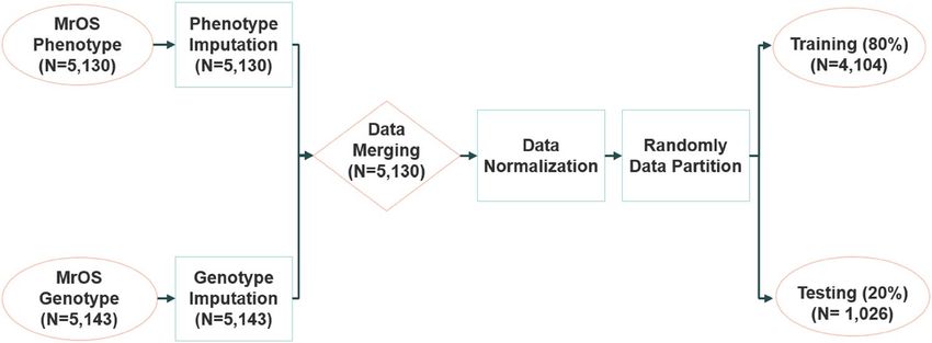
www.nature.com/scientificreports/
Training dataset Test dataset
Variable* (n = 4104) (n = 1026) p Value**
Femoral neck BMD (g/cm2) 0.78 ± 0.13 0.79 ± 0.13 0.61
Total hip BMD (g/cm2) 0.96 ± 0.14 0.96 ± 0.14 0.55
Total spine BMD (g/cm2) 1.07 ± 0.19 1.07 ± 0.19 0.36
Age (year) 73.77 ± 5.93 73.95 ± 5.83 0.78
Height (cm) 174.15 ± 6.81 174.16 ± 6.61 0.69
Weight (kg) 83.28 ± 13.46 82.73 ± 12.73 0.37
Alcohol use (drinks/week) 4.25 ± 6.87 3.98 ± 6.06 0.57
GRS*** 31.6 ± 0.44 31.59 ± 0.45 0.81
Impairment of instrumental activities of daily living 0.37 ± 0.88 0.36 ± 0.83 0.79
Walking speed (m/s) 1.07 ± 0.27 1.07 ± 0.27 0.53
Smoking, no. (%)
No 1535 (37.4%) 406 (39.6%)
0.41
Past 2430 (59.2%) 587 (57.3%)
Current 139 (3.4%) 32 (3.1%)
Race, no. (%)
White 3707 (90.3%) 909 (88.6%)
African American 141 (3.4%) 40 (3.9%)
0.11
Asian 120 (2.9%) 45 (4.4%)
Hispanic 87 (2.1%) 24 (2.3%)
Other 49 (1.2%) 8 (0.8%)
Table 1. Baseline characteristics of training and testing dataset. *Continuous variables were expressed as mean
± SD, and categorical variables were expressed as number (%). **p Value were obtained by t-test for continuous
variables and chi-square tests for the categorical variable. ***GRS: genetic risk score, which was calculated
based on 1103 BMD-related SNPs.
of osteoporosis, men suffer greater morbidity and mortality rates following osteoporotic fractures, especially at
an advanced age. With populations aging worldwide, osteoporosis is a critical public health problem globally.
For example, by 2050, Worldwide hip fracture incidence alone is projected to increase by threefold 10% in men
and twofold in women compared to 1990 d ata2. The potentially high cumulative rate of fracture, which often
ortality3, has caused an inevitable high social and economic burden associated
results in excess disability and m
with bone health.
BMD has been used to define osteoporosis since 1994. The World Health Organization defines osteoporosis
as a BMD that lies 2.5 or more standard deviations below the average value for young healthy women4. BMD
is the single strongest predictor of primary osteoporotic f racture5. Each standard deviation decrease in BMD is
associated with a 1.5 to threefold increase in fracture risk, depending on the skeletal region measured, type of
fracture, and ethnicity of the study p opulation6.
BMD is a highly heritable trait. Genetic differences in BMD are well documented7. Family and twin stud-
ies show BMD variances of 50–85% are attributable to genetic f actors8. Other studies report BMD heritability
estimates of 72–92%9. In the past decade, major genome-wide association studies (GWAS) and genome-wide
meta-analyses have successfully identified numerous BMD-associated Single Nucleotide Polymorphisms (SNPs)
associated with decreased BMD10. However, combining these large number of highly significant SNPs, surpris-
ingly, only explained a very small proportion of BMD variance11. Such inconsistency may be caused by limita-
tions of the conventional regression approaches employed as these traditional methods lack the flexibility and
adequacy of modeling complex interactions and regulations.
Machine learning (ML) focuses on implementing computer algorithms capable of maximizing predictive
accuracy from complex data. ML has an excellent capacity to model complex real-world relationships, including
variable interactions. ML techniques have been applied in clinical research for disease prediction, and ML has
shown much higher accuracy for diagnosis than conventional m ethods12. Gradient boosting, random forest, and
neural network are widely used ML approach for modeling complex medical d ata12. However, the performance
of these ML models for BMD prediction remains largely unknown, especially with genomic data.
Hence, the current study aims are (1) to develop models using ML algorithms to predict BMD from the data
with genomic variants, and (2) to compare these models to determine which ML model performs the best for
BMD prediction. We hypothesize that when we utilize the ML models to predict BMD, ML models will perform
better than the linear regression model.
Results
Baseline characteristics. Table 1 shows the characteristics of participants within the training (n = 4104)
and the test (n = 1026) datasets. Demographic and clinical variables were not significantly different in training
and test datasets. All BMD measurements from the femur neck, total spine, and total hip were normally distrib-
uted, with means of 0.78, 0.96, 1.07, and standard deviations 0.13, 0.14, 0.19, respectively. The Pearson correla-
Scientific Reports | (2021) 11:4482 | https://doi.org/10.1038/s41598-021-83828-3 2
Vol:.(1234567890)www.nature.com/scientificreports/
Figure 1. Mean square error (MSE) and mean absolute error (MAE) of different models in predicting various
BMD in training (n = 4104) and testing (n = 1026); GRS and phenotypic covariates were used as predictors.
Figure 2. Mean square error (MSE) and mean absolute error (MAE) of different models in predicting various
BMD in training (n = 4104) and testing (n = 1026); 1103 individual risk SNPs and phenotypic covariates were
used as predictors. Lasso regularization, with the penalized value of 0.01, was applied to linear regression.
tion between each BMD outcome and demographic/clinical variables ranged from − 0.19 to 0.41 (Table S1). In
the study data, 12%, 12%, and 13% of the 1103 SNPs were significantly associated with femoral neck, total hip,
and total spine BMD at the significance level α = 0.05, respectively.
Model performance. Figure 1 shows MSE and MAE for each model with phenotype covariate and GRS
as predictors. In the test dataset (n = 1026), MSE was similar between all models in each BMD outcome, and
the same results were observed for MAE. When we replaced GRS with 1103 individual SNPs in the predictors
(Fig. 2), ML models had smaller MSE than the linear model (with lasso regularization) in the testing dataset.
Similar results were observed with MAE. Overall, the gradient boosting model had the lowest MSE and MAE
in the testing dataset.
Figure 3 shows each model’s performance in the test dataset (n = 1026). The upper panel in Fig. 3 compared
model performance when using phenotype covariates and GRS as predictors. MSE in each model became similar
Scientific Reports | (2021) 11:4482 | https://doi.org/10.1038/s41598-021-83828-3 3
Vol.:(0123456789)www.nature.com/scientificreports/
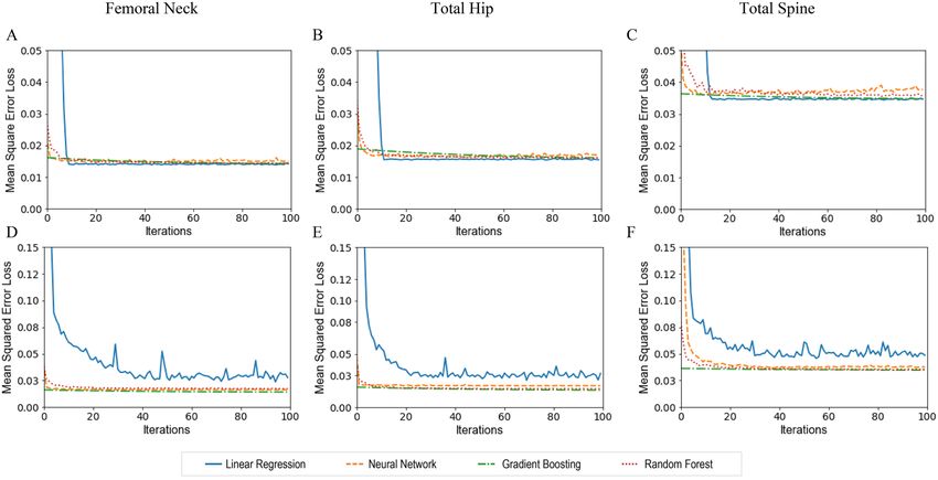
Figure 3. Mean squared error loss of various models with the number of training iterations for BMD prediction
in the test dataset (n = 1026). The upper panel shows the performance of each model with phenotype covariates
and GRS as predictors in predicting BMD at the femoral neck (A), total hip (B), and total spine (C) in the
testing dataset at different BMD sites. The lower panel shows the performance of each model with phenotype
covariates and 1103 individual SNPs in predicting BMD at the femoral neck (D), total hip (E), and total spine
(F). Lasso regularization with the penalized value of 0.01 was used in the linear regression model for 1103
individual SNPs and phenotype covariates.
in the test data with increased training iterations. Although the linear regression model had a relatively higher
MSE in the first few iterations, in the testing dataset, linear regression and ML models’ performance became
nearly identical with increased iterations in BMD measured from all three skeletal regions. All models had the
best performance at femur neck BMD (Fig. 3A), followed by total hip BMD (Fig. 3B) and then total spine BMD
(Fig. 3C). The lower panel in Fig. 3 compared model performance when using phenotype covariates and 1103
individual SNPs as predictors. MSE in linear regression (with lasso regularization) was much larger than that
in other ML models in the testing data. The results were consistent with BMD measured at the three different
skeletal regions.
We tested different hyper-parameters in each algorithm (Table S2) in the training data. We found that a
relatively small depth of the tree (depth = 5) was observed in random forest and gradient boosting when pheno-
type covariate and GRS were included as predictors in the model. However, relatively higher for random forest
(depth = 20) and gradient boosting (depth = 10) were obtained when phenotype covariate and 1103 individual
SNPs were included in the model. The optimal hyper-parameters in the neural network were obtained when
the batch size of 20, the first layer with 500 neurons, three hidden layers, and the sigmoid activation function
were used.
The coefficient determination ( R2) of each model was shown in Table S3. For each BMD outcome, the R2 in
models with 1103 individual risk SNPs and phenotypic covariates ranged from 8 to 18%. The R2 in the model
with GRS and phenotypic covariates ranged from 6 to 16%. In the testing data, the 1103 individual risk SNPs
contribute the variance of each BMD about 1–2% in Femoral Neck and Total Hip BMD and 2–4% in Total Spine
BMD, respectively (Table S3). The early stopping iteration in the training dataset for each model was shown in
Table S4. Fewer iterations were required for the model with phenotype covariate and GRS as predictors. However,
models with phenotype covariate and individual risk SNPs required more iterations for the training, especially
in linear regression (with lasso regularization).
To compare the performance between models that uses GRS and phenotype covariates as the predictors, we
used the nonparametric Wilcoxon signed-rank test results for multiple comparisons of MSE between models.
The results are shown in Table 2. With Bonferroni corrections for multiple comparisons (α = 0.05/6 = 0.0083),
none of the comparisons were statistically significant except the comparison between gradient boosting and
random forest at femur neck BMD and total spine BMD. However, as shown in Table 3, when using phenotype
covariates and 1103 SNPs as the predictors, the difference of MSE in most pairwise comparisons was statistically
significant with p < 0.0001. The only exceptions were the comparison between the neural network and random
forest at femur neck BMD and the comparison between the gradient boosting and random forest at total hip
BMD with p > 0.05.
Scientific Reports | (2021) 11:4482 | https://doi.org/10.1038/s41598-021-83828-3 4
Vol:.(1234567890)www.nature.com/scientificreports/
Linear regression Random forest Gradient boosting
Femoral neck BMD
Neural network > .05 > .05 > .05
Gradient boosting > .05 < .0001 –
Random forest > .05 – –
Total hip BMD
Neural network > .05 > .05 > .05
Gradient boosting > .05 > .05 –
Random forest > .05 – –
Total spine BMD
Neural network > .05 > .05 > .05
Gradient boosting > .05 < .01 –
Random forest > .05 – –
Table 2. Statistical comparisons of mean square errors in the testing dataset (n = 1026) between various
models when phenotype covariates and GRS were used as the predictors. The Wilcoxon Signed-Rank Test was
used to determine all p values.
Linear regression* Random forest Gradient boosting
Femoral neck BMD
Neural network < .0001 > .05 < .0001
Gradient boosting < .0001 < .0001 –
Random forest < .0001 – –
Total hip BMD
Neural network < .0001 < .0001 < .0001
Gradient boosting < .0001 > .05 –
Random forest < .0001 – –
Total spine BMD
Neural network < .0001 < .0001 < .0001
Gradient boosting < .0001 < .001 –
Random forest < .0001 – –
Table 3. Statistical comparisons of mean square errors in the testing dataset (n = 1026) between various
models when phenotype covariates and 1103 SNPs were used as the predictors. The Wilcoxon Signed-Rank
Test was used to determine all p values. *Lasso regularization with the penalized value of 0.01 was used in the
linear regression.
Discussion
This study presents findings from employing various ML models and linear regression, as well as genotype and
phenotype data for BMD prediction in older men. Interestingly, we found that if we use GRS—that is, the sum-
marized genetic risk from associated SNPs—as the genetic predictor in the model, all ML approaches did not
perform better than linear regression in predicting BMD. In contrast, if we replace GRS with the 1103 individual
risk SNPs as predictors in the model, ML models all had significantly better performance than linear regres-
sion for BMD prediction. With the increasing availability of genomic and health big data, ML technologies,
which employ a wide-ranging class of algorithms, have increasingly been utilized effectively in medical research,
especially in disease prediction. However, our study findings suggested that the conventional approach may be
sufficient if we use GRS, a summary metric for genetic risk, as the genetic predictor in the prediction model. In
contrast, our study suggests that ML approaches instead may be recommended if a large number of individual
genetic variants are included as predictors.
ML models have been used widely for prediction in classification problems, especially for disease prediction.
However, studies that utilized ML technologies to predict quantitative traits are still rare. Reportedly, artificial
neural networks were utilized for BMD prediction in a small sample of Japanese postmenopausal women, using
common risk factors and a BMD previously measured13. However, to the best of our knowledge, our study is
the first attempt to predict BMD using both advanced ML approaches and genomic information, as well as the
first to identify the best ML model for BMD prediction. Our study demonstrated that ML technologies perform
better than conventional methods for predicting quantitative traits in complex data that include a large number
of genomic variants as predictors.
Risk SNPs identified in GWAS and genome-wide meta-analyses have posed a challenge in conventional sta-
tistical analysis because their effect size is very small. Each associated SNP contributes minimally to the variance
Scientific Reports | (2021) 11:4482 | https://doi.org/10.1038/s41598-021-83828-3 5
Vol.:(0123456789)www.nature.com/scientificreports/
of BMD. Thus, GRS is widely used to integrate the effects of individual associated SNPs into a single genetic
summary variable for prediction research in many studies. Although such an approach improves the prediction
ability, many uncertainties remain. For example, this approach does not account for gene interaction and regula-
tion. To address these limitations, we utilized ML approaches in the current study so that individual SNPs can
be included to replace GRS in the modeling process. ML approaches have the capacity to handle high dimension
data and incorporate the various nonlinear interactions between genetic variants/predictors, which cannot be
addressed by conventional modeling methods. Thus, ML approaches provide great potential for improving BMD
prediction. In the present study, we employed random forest, gradient boosting, and neural networks, as well
as 1103 individual related SNPs, to find a more accurate BMD prediction model. We found that the gradient
boosting model performs best in predicting BMD as it has the lowest MSE and MAE, and the highest coefficient
of determination in the validation for all three BMD outcomes.
Studies14,15 show that the recursive partitioning approaches such as the random forest and gradient boost-
ing have been used to detect genetic loci interaction for the phenotypic o utcome16–19. The highest predictive
performance of the gradient boosting model has been utilized widely in predicting various diseases and out-
comes, including hip f ractures20, sepsis21, urinary tract infections22, hepatocellular c arcinoma23, and bioactive
molecules24. The present study suggested that the gradient boosting approach, combined with individual SNPs
as the predictors and considering the interaction of SNPs, can provide a more accurate BMD prediction.
Our study has several strengths. To ensure that our study results were robust, we took the following strategies.
First, we have used two metrics, MSE and MAE, to examine and compare the prediction accuracy of the four
models we developed. The study findings were consistent between analyses using the two metrics. Second, we
performed data analysis separately for the outcome variable BMD measured in three different skeletal regions.
The study results were consistent. Finally, we employed the nonparametric Wilcoxon signed-rank test to examine
the significance of the different MSE and MAE between any two models so as to ensure the data distribution did
not bias the results of the statistical test. We also used Bonferroni corrections for the multiple comparisons in
order to ensure our conclusions were robust.
However, our study has some limitations as well. First, the study sample size (n = 5130) is relatively small
for ML methods. ML methods often require a much larger sample size for training. To address this limitation,
we used tenfold cross-validation for tuning the hyper-parameters within the training dataset. Therefore, we did
not need to allocate part of the study sample for model validation, maximizing the sample size training model.
Second, some covariates were not available in the MrOS through dbGaP, including related medications, comor-
bidities, and physical activities. Lacking these phenotypic variables could have impacted the performance of all
prediction models. Third, the MrOS data only included men ≥ 65 years old and mostly Caucasian (90%), so
findings from the present study may not apply to women, younger individuals, or other ethnicities. Finally, rare
risk SNPs were less likely to be included for modeling in this study because risk SNPs used in this study were
identified from a GWAS study, which likely discovered common but not rare v ariants25. Nevertheless, these
limitations are unlikely to have altered our findings in the current study because this is a self-controlled study,
with all models developed and validated by the same datasets.
In summary, there was not a significant difference in predicting BMD between various ML models and linear
regression if GRS, a metric used to summarize genetic variants, was used for model development. However, when
using many individual SNPs as predictors to replace GRS, ML models performed significantly better than linear
regression in BMD prediction. Among these ML models, the gradient boost model performed best for BMD
prediction. Our study suggests that ML models, especially gradient boosting, can be used to identify patients
with low BMD if their genetic information is available. Our study also suggested that when researchers used a
large number of genetic variants or other predictors, ML approaches, especially gradient boosting, should be
considered. Additionally, more comprehensive studies, especially those including women, young participants,
rare genetic variants, and additional risk factors, are warranted to examine further and advance the research
findings of the present study.
Materials and methods
Data source. The Osteoporotic Fractures in Men Study (MrOS) was used as the data source for this study.
MrOS is a federal funded prospective cohort study that was designed to investigate anthropometric, lifestyle,
and medical factors associated with bone health in older, community‐dwelling men. Details of the MrOS study
design, recruitment, and baseline cohort characteristics have been reported elsewhere26. With the approval of
the institutional review board at the University of Nevada, Las Vegas, and the National Institute of Health (NIH),
the genotype and phenotype data of MrOS were acquired from dbGaP (Accession: phs000373.v1.p1). MrOS
consisted of 5130 subjects, all of whom had genotype and phenotype data available for authorized access. All
participants provided written informed consent in participating in this study, and all research was performed
following relevant guidelines/regulations.
Study participants. Participants in the MrOS were at least 65 years old, community-dwelling, ambulatory,
and had not received bilateral hip replacement27 at the study entry. At enrollment, participants had to provide
self-reported data, understand and sign the written informed consent, complete the self-administered question-
naire, attend a clinic visit, and complete the anthropometric, DEXA vertebral X-ray procedures. The participants
could not have a medical condition that would result in imminent death, which was based on the investigators’
judgment. A total of 5994 men were enrolled between March 2000 and April 2002, all of whom were from six
communities in the United States (Birmingham, AL; Minneapolis, MN; Palo Alto, CA; Pittsburgh, PA; Portland,
OR; and San Diego, CA.)28.
Scientific Reports | (2021) 11:4482 | https://doi.org/10.1038/s41598-021-83828-3 6
Vol:.(1234567890)www.nature.com/scientificreports/
Figure 4. Overview of data process flow.
Outcome BMD measurements. Total body, total femur BMD, and lumbar spine (L1 to L4) were meas-
ured using a fan-beam dual-energy X-ray absorptiometry (QDR 4500 W, Hologic, Inc., Bedford, MA, USA) at
the second visit of MrOS. Participants were scanned for BMD measurements by licensed densitometrists, using
standardized procedures. All DXA operators were centrally certified, based on the evaluation results of scanning
and analysis techniques. Cross-calibrations conducted before participants’ visits for BMD measurement found
no linear differences across scanners. The maximum percentage difference between scanners was 1.4% in mean
BMD of the total s pine29. No shifts or drifts in scanner performance was found, based on daily quality control
in each clinical center.
Assessment of covariates. Bone health-related information, including demographics, clinical history,
medications, and lifestyle factors, was obtained by self-administered questionnaires. The information collected
contained the variables used in this study, including age, race, smoking, and alcohol consumption. Height (cm)
was measured using a Harpenden stadiometer, and weight (kg) was measured by a standard balance beam or an
electric scale.
Smoking was categorized as “never,” “past,” and “current.” Alcohol intake was quantified in terms of the usual
number of drinks per day. Walking speed was determined by timed completion of a 6-m course, performed at
each participant’s typical walking speed. Mobility limitations were quantified by using a participant’s ability to rise
from a chair without using his arms and his ability to complete five chair stands. Each participant’s function status
was quantified by assessing daily living difficulty on a scale of 0–3, with five instrumental activities of daily living,
which include walking on level ground, climbing steps, preparing meals, performing housework, and shopping.
Genotyping data. Whole blood samples at the baseline were used for DNA extraction. Consent for DNA
use was obtained through written permission. Quality-control genotype data files were acquired through dbGaP
and implemented with P LINK30. Genotype imputation was conducted at the Sanger Imputation S erver31. The
Haplotype Reference Consortium imputation reference p anel32 and the Positional Burrows–Wheeler Transform
imputing algorithm33 were used to ensure high quality of genotype imputation. Based on the study published by
Morris et al. in 2019, a total of 1103 associated SNPs were extracted for this a nalysis10. These 1103 SNPs were con-
ditionally independent at genome-wide significance (p < 6.6 × 10⁻⁹ ) with BMD estimated by heel quantitative
ultrasound (eBMD)10. All the 1103 SNPs were successfully imputed in the MrOS data and were included in the
analysis. The imputation quality was excellent, with a mean R2 of 0.99. The Chi-square test was used to examine
the correlations between these SNPs in the study population, and we found that 58% of these SNPs are not inde-
pendent. Among the SNPs that are not independent (635 SNPs, 58%) in the Lasso linear regression model, the
estimated coefficients of 88% SNPs (59) became zero, which were eliminated in the final linear regression model.
The Analysis of Variance test34 was employed to examine the association between each SNP and each BMD
outcome. Genotyping for MrOS samples was performed with the Illumina HumanOmni1_Quad_v1-0 H array.
A total of autosomal 934,940 SNPs passed the quality control with the following criteria: minor allele frequency
≥ 0.05 individual missingness < 5%, SNPs call rate > 95%, and Hardy–Weinberg equilibrium p value < 0.0001.
Genetic risk score. A genetic risk score (GRS) is a standardized metric that allows the composite assess-
ment of genetic risk in complex traits. The GRS was derived from the number of risk alleles and their effect
size for each study subject. We performed a linkage disequilibrium (LD) pruning in advance to eliminate pos-
sible LD between SNPs; however, none of the SNPs were eligible for removal during the pruning process. The
weighted GRS was then calculated with the algorithms described previously35. Briefly, for each participant in
MrOS, weighted GRS was calculated by summing the number of risk alleles at each locus weighted by regression
coefficients related to BMD10.
Data processing. Figure 4 shows an overview of our data process flow for this study. After genotype impu-
tation, the phenotype data set (n = 5130) and genotype data set (n = 5143) were merged, and 13 participants were
removed from the analysis due to the lack of all phenotype data. After combining the data set, each phenotype
Scientific Reports | (2021) 11:4482 | https://doi.org/10.1038/s41598-021-83828-3 7
Vol.:(0123456789)www.nature.com/scientificreports/
variable has less than 1% missing value in 5130 participants. One participant has a missing value of femoral neck
and total hip BMD, and ten participants have a missing value of total spine BMD. All other variables do not have
the missing value. We normalized all continuous variables in the data, then randomly divided the dataset into a
training set (80%, n = 4104) and a test set (20%, n = 1026). The median i mputation36, the most common imputa-
tion method for continuous variables, was used to replace missing values in the data, maximizing the sample
size for analysis.
Data analysis. The outcome variables were BMD measured from various skeletal regions, which included
femoral neck, total spine, and total hip. The predictors included GRS, age, race, body weight, height, smoking,
alcohol consumption, walking speed, impairment of instrumental activities of daily living, and mobility limita-
tions. Linear regression, random forest, gradient boosting, and neural network with backpropagation were used
to train the model separately. The neural network with backpropagation consists of three sequential layers: input,
hidden, and output. The number of hidden layers was considered as the hyper-parameters in this s tudy37. Lasso
regularization, with the penalized value of 0.01, was used to address the overfitting problem in the first layer of
the neural network model38. The rectified linear unit, Sigmoid, and Hyperbolic tangent activation functions were
considered39. We also conducted analyses that replaced the GRS with the 1103 individual SNPs in each model.
We encoded each risk SNP as three different genotypes (dominant homozygous allele, heterozygotes, homozy-
gous minor allele) with 0, 1, and 2.
In model training, tenfold cross-validation was used for hyper-parameter optimization. We divided the train-
ing set into 10-folds, and chose one fold as a validation set, with the remaining folds used as the training set. We
used Scikit-learn’s randomized search cross-validation40 to find the best hyperparameters for different algorithms.
To avoid the high computational burden in searching for all the possible parameters, we utilized randomized
search cross-validation to find the optimal hyper-parameters by sampling a different combination of parameters
from the given distribution41. The training set was used to train and construct linear regression models, random
forest, gradient boosting, and neural networks. For linear regression modeling, as multicollinearity may occur
when including 1103 individual SNPs in the model as predictors, we implemented the three shrinkage methods
of Lasso42, Ridge r egression43, and Elastic N
et44 separately for the linear regression model. We found that lasso
regularization with the penalized value of 0.01 showed the lowest error rate in the linear regression model. For
each other type of ML, we tested different combinations of hyper-parameters in the training sets to obtain the
most optimal model for each ML (Table S2). Each combination of various hyper-parameters was evaluated by
the mean squared error or mean absolute error of the model. For each type of ML, the set of parameters with the
lowest mean squared error or mean absolute error in the testing data was selected. The early stopping criteria of
ML training were defined as no decrease in the MSE or MAE by 0.001 in the training data set of 100 consecutive
iterations. The early stopping procedure was applied in each 10-folds cross-validation of training dataset and
each early stopping iteration number was recorded. Then, the average early stopping iteration was calculated
for each model.
The testing set (20%) was used to evaluate the prediction performance of the developed model. Metrics for
model performance
evaluation are mean squared e rror45, mean absolute e rror46, and the coefficient of determi-
nation R2 47. We adopted two metrics:
• Mean Squared Error (MSE):
n
1
2
MSE = yi − y
i
n
i=1
• Mean Absolute Error (MAE):
n
1
MAE = |yi − y
i |
n
i=1
where n is the sample size, yi is the actual value for each observation, and y i is the estimated value for each
observation from the model. We first used MSE as a loss function to develop the model in a training set. We also
calculated MSE for each model in the test set and used the MSE for model evaluation. We then reanalyzed the
data by replacing MSE with MAE, in which MAE was used as a loss function to develop the model in a training
set and was calculated in the test set for model evaluation. We also calculated the coefficient of determination for
each model in the training and testing dataset. Wilcoxon signed-rank test was employed to examine the difference
of MSE or MAE between ML models because the data distribution assumption for the student t-test was not met.
All of the analyses were performed in the Python Software Foundation and Python Language Reference, version
3.7.3, with the package Scikit-learn: Machine Learning in P ython40, and the glmnet48 packages of R software was
used for Lasso, Ridge regression, and Elastic Net.
Data availability
The data/analyses presented in the current publication are based on the use of study data downloaded from
the dbGaP website under phs000373.v1.p1 (https://www.ncbi.nlm.nih.gov/projects/gap/cgi-bin/study.cgi?study
_id=phs000373.v1.p1). The code required for replicating the results reported in this paper is available at https
://github.com/wulabunlv/BMD_ML.
Scientific Reports | (2021) 11:4482 | https://doi.org/10.1038/s41598-021-83828-3 8
Vol:.(1234567890)www.nature.com/scientificreports/
Received: 12 June 2020; Accepted: 9 February 2021
References
1. Cummings, S. R. & Melton, L. J. Epidemiology and outcomes of osteoporotic fractures. Lancet 359, 1761–1767 (2002).
2. Gullberg, B., Johnell, O. & Kanis, J. A. World-wide projections for hip fracture. Osteoporos. Int. 7, 407–413 (1997).
3. Melton, L. J. & Cooper, C. Chapter 21—Magnitude and Impact of Osteoporosis and Fractures. in Osteoporosis 557–567 (Academic
Press Inc., 2007). https://doi.org/10.1016/B978-012470862-4/50022-2
4. Cosman, F. et al. Clinician’s guide to prevention and treatment of osteoporosis. Osteoporos. Int. 25, 2359–2381 (2014).
5. Kanis, J. A. et al. Assessment of fracture risk. Osteoporos. Int. 16, 581–589 (2005).
6. Marshall, D. & Wedel, H. Meta-analysis of how well measures of bone mineral density predict occurrence of osteoporotic fractures.
BMJ 312, 1254–1259 (1996).
7. Warrington, N. M., Kemp, J. P., Tilling, K., Tobias, J. H. & Evans, D. M. Genetic variants in adult bone mineral density and fracture
risk genes are associated with the rate of bone mineral density acquisition in adolescence. Hum. Mol. Genet. 24, 4158–4166 (2015).
8. Eisman, J. A. Genetics of osteoporosis. Endocr. Rev. 20, 788–804 (1999).
9. Pocock, N. A. et al. Genetic determinants of bone mass in adults. A twin study. J. Clin. Investig. 80, 706–710 (1987).
10. Morris, J. A. et al. An atlas of genetic influences on osteoporosis in humans and mice. Nat. Genet. 51, 258–266 (2019).
11. Xiao, X., Roohani, D. & Wu, Q. Genetic profiling of decreased bone mineral density in an independent sample of Caucasian women.
Osteoporos. Int. 29, 1807–1814 (2018).
12. Hsieh, C. H. et al. Novel solutions for an old disease: Diagnosis of acute appendicitis with random forest, support vector machines,
and artificial neural networks. Surgery 149, 87–93 (2011).
13. Shioji, M. et al. Artificial neural networks to predict future bone mineral density and bone loss rate in Japanese postmenopausal
women. BMC Res. Notes 10, 1–5 (2017).
14. Cordell, H. J. Detecting gene-gene interactions that underlie human diseases. Nat. Rev. Genet. 10, 392–404 (2009).
15. Heidema, A. G. et al. The challenge for genetic epidemiologists: How to analyze large numbers of SNPs in relation to complex
diseases. BMC Genet. 7, 23 (2006).
16. Zhang, H. & Bonney, G. Use of classification trees for association studies. Genet. Epidemiol. 19, 323–332 (2000).
17. Evans, D. M. Gene–Gene Interaction and Epistasis. Analysis of Complex Disease Association Studies (Elsevier Inc., 2011). https://
doi.org/10.1016/B978-0-12-375142-3.10012-4
18. Nelson, M. R., Kardia, S. L. R., Ferrell, R. E. & Sing, C. F. A combinatorial partitioning method to identify multilocus genotypic
partitions that predict quantitative trait variation. Genome Res. 11, 458–470 (2001).
19. Hussain, D. & Han, S. M. Computer-aided osteoporosis detection from DXA imaging. Comput. Methods Progr. Biomed. 173,
87–107 (2019).
20. Kruse, C., Eiken, P. & Vestergaard, P. Machine learning principles can improve hip fracture prediction. Calcif. Tissue Int. 100,
348–360 (2017).
21. Chiew, C. J. et al. Heart rate variability based machine learning models for risk prediction of suspected sepsis patients in the
emergency department. Medicine (Baltimore) 98, e14197 (2019).
22. Taylor, R. A., Moore, C. L., Cheung, K. H. & Brandt, C. Predicting urinary tract infections in the emergency department with
machine learning. PLoS ONE 13, 1–15 (2018).
23. Sato, M. et al. Machine-learning approach for the development of a novel predictive model for the diagnosis of hepatocellular
carcinoma. Sci. Rep. 9, 1–7 (2019).
24. Babajide Mustapha, I. & Saeed, F. Bioactive molecule prediction using extreme gradient boosting. Molecules 21, 1–11 (2016).
25. Nguyen, T. V. & Eisman, J. A. Genetic profiling and individualized assessment of fracture risk. Nat. Rev. Endocrinol. 9, 153–161
(2013).
26. Orwoll, E. et al. Design and baseline characteristics of the osteoporotic fractures in men (MrOS) study—A large observational
study of the determinants of fracture in older men. Contemp. Clin. Trials 26, 569–585 (2005).
27. Riggs, L. & Melton, L. The worldwide problem of osteoporosis: Lessons from epidemiology. Bone 17, 2–3 (1995).
28. Blank, J. B. et al. Overview of recruitment for the osteoporotic fractures in men study (MrOS). Contemp. Clin. Trials 26, 557–568
(2005).
29. Cauley, J. A. et al. Factors associated with the lumbar spine and proximal femur bone mineral density in older men. Osteoporos.
Int. 16, 1525–1537 (2005).
30. Purcell, S. et al. PLINK: A tool set for whole-genome association and population-based linkage analyses. Am. J. Hum. Genet. 81,
559–575 (2007).
31. Das, S. et al. Next-generation genotype imputation service and methods. Nat. Genet. 48, 1284–1287 (2016).
32. Loh, P. R. et al. Reference-based phasing using the Haplotype Reference Consortium panel. Nat. Genet. 48, 1443–1448 (2016).
33. Durbin, R. Efficient haplotype matching and storage using the positional Burrows–Wheeler transform (PBWT). Bioinformatics
30, 1266–1272 (2014).
34. Pitman, A. E. J. G. Significance tests which may be applied to samples from any populations III.* The analysis of variance test.
Biometrika 29, 322–335 (1938).
35. Andrews, N. A. Genome-wide association studies in the osteoporosis field: Impressive technological achievements, but an uncertain
future in the clinical setting. IBMS Bonekey 7, 382–387 (2010).
36. Gao, B. Advances in Intelligent Systems and Computing Vol. 997 (Springer, Berlin, 2019).
37. Claesen, M. & De Moor, B. Hyperparameter Search in Machine Learning. arXiv 10–14 (2015).
38. Amoroso, N. et al. Deep learning and multiplex networks for accurate modeling of brain age. Front. Aging Neurosci. 11, 1–12
(2019).
39. Nair, V. & Hinton, G. E. Rectified linear units improve restricted Boltzmann machines. Proceeding 27th Int Conf Mach Learn
807–814 (2010). https://doi.org/10.1123/jab.2016-0355
40. Pedregosa, F. et al. Scikit-learn: Machine learning in Python. J. Mach. Learn. Res. 12, 2825–2830 (2011).
41. Bergstra, J. & Bengio, Y. Random search for hyper-parameter optimization. J. Mach. Learn. Res. 13, 281–305 (2012).
42. Tibshirani, R. Regression shrinkage and selection via the lasso. J. R. Stat. Soc. Ser. B 58, 267–288 (1996).
43. Hoerl, A. E. & Kennard, R. W. Ridge regression: Biased estimation for nonorthogonal problems. Technometrics 12, 55–67 (1970).
44. Zou, H. & Hastie, T. Regularization and variable selection via the elastic net. J. R. Stat. Soc. Ser. B Stat. Methodol. 67, 301–320
(2005).
45. Mean Squared Error. in Encyclopedia of Machine Learning (eds. Sammut, C. & Webb, G. I.) 653 (Springer US, 2010). https://doi.
org/10.1007/978-0-387-30164-8_528
46. Mean Absolute Error. in Encyclopedia of Machine Learning (eds. Sammut, C. & Webb, G. I.) 652 (Springer US, 2010). https://doi.
org/10.1007/978-0-387-30164-8_525
47. Nagelkerke, N. J. D. A note on a general definition of the coefficient of determination. Biometrika 78, 691–692 (1991).
48. Mohammadi, R. & Wit, E. C. Regularization paths for generalized linear models via coordinate descent. J. Stat. Softw. 33, 1–22
(2010).
Scientific Reports | (2021) 11:4482 | https://doi.org/10.1038/s41598-021-83828-3 9
Vol.:(0123456789)www.nature.com/scientificreports/
Acknowledgements
The research and analysis described in the current publication were supported by the Genome Acquisition and
Analytics (GAA) Research Core of the Personalized Medicine Center of Biomedical Research Excellence in the
Nevada Institute of Personalized Medicine. The National Supercomputing Institute at the University of Nevada
Las Vegas provided bioinformatical analysis facilities for this study.
Author contributions
Conceptualization: Q.W.; methodology: Q.W., F.N., J.J., and B.B.; software: J.J. and B.B.; validation: Q.W., F.N., J.J.,
B.B., M.H., R.G. and K.S.; formal analysis: J.J. and B.B.; investigation: Q.W., F.N., J.J., B.B., M.H., R.G. and K.S.;
resources: Q.W.; data curation: J.J. and B.B.; writing—original draft preparation: Q.W., and J.J.; writing—review
and editing: Q.W., F.N., J.J., M.H., R.G. and K.S.; visualization: J.J. and B.B.; supervision, Q.W.; project administra-
tion: Q.W.; funding acquisition: Q.W. All authors have read and agreed to the published version of the manuscript.
Funding
The research and analysis described in the current publication were supported by a grant from the National
Institute of General Medical Sciences (P20GM121325) and a grant from the National Institute on Minority
Health and Health Disparities (R15MD010475). The funding sponsors were not involved in the analysis design,
genotype imputation, data analysis, interpretation of the analysis results, or the preparation, review, or approval
of this manuscript.
Competing interests
The authors declare no competing interests.
Additional information
Supplementary Information The online version contains supplementary material available at https://doi.
org/10.1038/s41598-021-83828-3.
Correspondence and requests for materials should be addressed to Q.W.
Reprints and permissions information is available at www.nature.com/reprints.
Publisher’s note Springer Nature remains neutral with regard to jurisdictional claims in published maps and
institutional affiliations.
Open Access This article is licensed under a Creative Commons Attribution 4.0 International
License, which permits use, sharing, adaptation, distribution and reproduction in any medium or
format, as long as you give appropriate credit to the original author(s) and the source, provide a link to the
Creative Commons licence, and indicate if changes were made. The images or other third party material in this
article are included in the article’s Creative Commons licence, unless indicated otherwise in a credit line to the
material. If material is not included in the article’s Creative Commons licence and your intended use is not
permitted by statutory regulation or exceeds the permitted use, you will need to obtain permission directly from
the copyright holder. To view a copy of this licence, visit http://creativecommons.org/licenses/by/4.0/.
© The Author(s) 2021
Scientific Reports | (2021) 11:4482 | https://doi.org/10.1038/s41598-021-83828-3 10
Vol:.(1234567890)You can also read