Star-Galaxy Separation via Gaussian Processes with Model Reduction
←
→
Page content transcription
If your browser does not render page correctly, please read the page content below
Star-Galaxy Separation via Gaussian Processes with Model Reduction

                                                                                          Imène R. Goumiri
                                                                      Physics Division, Lawrence Livermore National Laboratory
                                                                                      Amanda L. Muyskens
                                                                   Engineering Division, Lawrence Livermore National Laboratory

                                                                                        Michael D. Schneider
                                                                      Physics Division, Lawrence Livermore National Laboratory
arXiv:2010.06094v1 [astro-ph.IM] 13 Oct 2020

                                                                                      Benjamin W. Priest
                                                       Center for Applied Scientific Computing, Lawrence Livermore National Laboratory

                                                                                        Robert E. Armstrong
                                                                      Physics Division, Lawrence Livermore National Laboratory
                                                                                                LLNL-CONF-813954

                                                                                                    ABSTRACT

                                               Modern cosmological surveys such as the Hyper Suprime-Cam (HSC) survey produce a huge volume of low-resolution
                                               images of both distant galaxies and dim stars in our own galaxy. Being able to automatically classify these images is
                                               a long-standing problem in astronomy and critical to a number of different scientific analyses. Recently, the challenge
                                               of “star-galaxy” classification has been approached with Deep Neural Networks (DNNs), which are good at learning
                                               complex nonlinear embeddings. However, DNNs are known to overconfidently extrapolate on unseen data and require
                                               a large volume of training images that accurately capture the data distribution to be considered reliable. Gaussian Pro-
                                               cesses (GPs), which infer posterior distributions over functions and naturally quantify uncertainty, haven’t been a tool
                                               of choice for this task mainly because popular kernels exhibit limited expressivity on complex and high-dimensional
                                               data.
                                               In this paper, we present a novel approach to the star-galaxy separation problem that uses GPs and reap their benefits
                                               while solving many of the issues traditionally affecting them for classification of high-dimensional celestial image
                                               data. After an initial filtering of the raw data of star and galaxy image cutouts, we first reduce the dimensionality of
                                               the input images by using a Principal Components Analysis (PCA) before applying GPs using a simple Radial Basis
                                               Function (RBF) kernel on the reduced data. Using this method, we greatly improve the accuracy of the classification
                                               over a basic application of GPs while improving the computational efficiency and scalability of the method.

                                                                                              1.   INTRODUCTION

                                               Modern telescopes have enabled the capture of heretofore undetectable faint stars and galaxies. Recent large-scale
                                               surveys, like the Dark Energy Survey (DES) [20, 1] and the Hyper Surpime-Cam (HSC) [14, 2] survey, have generated
                                               vast quantities of data at increasing depths, requiring the development of automated algorithms to distinguish stars
                                               from galaxies. For bright objects the problem is usually fairly straightforward; however for fainter objects the problem
                                               becomes more difficult. At the depths of modern ground-based surveys faint galaxies are almost indistinguishable from
                                               point-like sources. Observations from space, where the resolution is better can significantly improve classification, but
                                               telescope time is too costly to observe large regions of the sky. Another factor is that the number of stars quickly
                                               decreases as a function of magnitude.
                                               Previous studies have applied several different approaches to star-galaxy separation. The morphological approach [21,
                                               19] uses the difference in shape in comparison with the point-spread function (PSF). This approach typically uses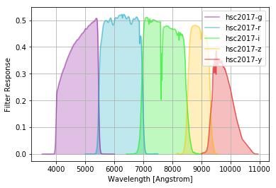
summary information to reduce the complexity of the problem as the number of pixels for different filters and PSF can
be high-dimensional. A similar morphological approach is used in both DES and HSC where a comparison of the flux
ratio of a galaxy model to a model using the PSF is used. An alternative approach uses the fact that stars and galaxies
have different spectral energy distributions. This translates into stars and galaxies clustering into different regions of
color space. For example, Pollo, A. et al. [17] used selections in color-color space for separation in far-infrared data.
There is also a rich literature of feature based machine learning solutions using color and morphological information as
input into decision trees [22, 18], neural networks [15] and ensemble methods such as random forests [11]. Although
decision tree-based models offer convenient interpretability features, they often generalize poorly and are sensitive to
crafted feature vectors, usually based upon expert knowledge in applications. Given the high dimensionality of the
data to be processed and the difficulty encountered in capturing generalizable data features using expert knowledge,
it is tempting to instead learn an appropriate feature representation. Representation learning models include deep
neural networks (DNNs) and kernel methods such as support vector machines (SVMs) and Gaussian processes (GPs).
Indeed, Odewahn et al. [16] applied shallow neural networks to the star–galaxy separation problem as early as 1992.
Recently, deep convolutional neural networks (CNNs) have achieved success in many areas of image classification due
to their success in capturing local interactions in structured pixel data [12]. Kim and Brunner [10] recently utilized
CNNs to demonstrate star-galaxy separation performance that was competitive with a conventional random forest-
based classifier [11].
In spite of their surprising generalization success in many problems, DNNs tend to poorly quantify their own uncer-
tainty [4, 8]. Importantly, this leads to overconfidently extrapolating on data that is far from training examples [9].
Overconfident extrapolation presents a significant problem to an automated classification pipeline, where one desires
to detect low-confidence predictions for possible human intervention. For example, the removal of ambiguous sources
to reduce systematic biases is a major issue facing the statistical analysis of astrophysical populations. Practitioners
often attempt to ameliorate the generalization gap by way of data augmentation and the use of very large labeled
datasets that covers the full data distribution. However, both mitigations introduce additional cost and implementation
complexity when training a model. For many astronomical applications, it is also not feasible to simulate unbiased
and complete training data distributions because the distributions are unknown (indeed, learning these distributions is
a primary scientific objective of many surveys).
Kernel-based representations learning methods present a nonparametric alternative to DNNs. A kernel learning model
poses a possibly nonlinear feature map from the data space to a latent reproducing kernel Hilbert space and reasons over
inner products in the latent space to make predictions. Unlike DNNs, which explicitly construct their feature maps,
kernel methods instead directly rely on the unique kernel function of their Hilbert space and do not compute their
feature maps explicitly. Fadely et al. [7] demonstrated the application of simple SVMs to the star–galaxy separation
problem. Gaussian processes (GPs) are a particularly attractive kernel model in many applications because they
support fully-Bayesian inference, which naturally affords disciplined uncertainty quantification by way of examining
the variance of the posterior distribution of a prediction. However, GPs have not yet been adopted in the star–galaxy
separation literature, most likely because popular kernel functions are known to implicitly utilize feature maps that are
less expressive than those produced by CNNs, particularly on high-dimensional image data [6].
We demonstrate an application of GPs to the star–galaxy separation problem that ameliorates expressivity issues by
first embedding high-dimensional image data onto a small number of their principle components using PCA. We show
that our augmented GP model demonstrates significant improvements over a naı̈ve GP on cosmological survey data,
even when using the simple RBF kernel. We also demonstrate superlinear computational savings using PCA over the
naı̈ve application. Our results motivate the serious consideration of GPs in star–galaxy separation as well as other
large-scale cosmological machine learning problems.

                                                    2.   THE DATA

We consider data from the first public release of the HSC Subaru Strategic Program [2]. HSC is the deepest ongoing
large-scale survey and provides an invaluable early testbed for algorithms being developed for the future Vera Rubin
Observatory1 . The HSC pipeline includes high level processing steps that generate coadded images and science-ready
catalogs. More details on the software that was used to process the data can be found in [5].
  1 https://www.lsst.org/
We create a training set of galaxy and star images from the UltraDeep COSMOS field. The COSMOS field is smaller in area but was observed many more times making the it significantly deeper than the main survey. It also overlaps space-based imaging from the Hubble Space Telescope (HST) where the resolution is much better. Leauthaud et al. [13] use HST images of the COSMOS field to separate stars and galaxies. The authors identify stars by looking for the stellar locus in the 2-d space of magnitude and peak surface brightness. They further claim their classification to be reliable up to magnitude ∼ 25. The classification breaks down at fainter magnitudes as point sources and galaxies appear identical. We cross match the HSC objects to the HST objects to label which object is a star or galaxy. The HSC data is quite a bit deeper (∼ 27 in the i filter), so we must be careful in interpreting results at the faint end. We show in Fig. 1 two examples of images (galaxy vs star) obtained from the data. Fig. 1: Example of images of a galaxy (left) and a star (right) from the HSC survey. Both images are composites where the RGB channels correspond to the z, i, and r filters respectively. Other examples can be much harder to differentiate. The HSC has five different filters, g, r, i, z, and y, corresponding to different frequency bands, as shown in Fig. 2. The y band data is not used because it is significantly shallower than the other bands. We extract images for each filter from the deblended HSC images. In an attempt to remove spurious sources, and to more closely match the HST catalogs, we only select objects with signal-to-noise ratio greater than 10 in all bands. While this cut does remove some artifacts, we find that our catalogs still contains too many junk objects. In addition to the signal-to-noise cut, we filter out images which fail the following test: the ratio of the χ 2 value for a circular area of interest (r < 2 FWHMPSF ) over the chi squared value of an annulus region around it (5 FWHMPSF < r < 10 FWHMPSF ) must be lower than 4, where FWHMPSF is the Full Width at Half Maximum (FWHM) of the Point Spread Function (PSF). Fig. 2: Different filters correspond to different frequency bands. For this analysis we used only images that had a signal to noise ratio greater than 10 in all bands.
3. METHODOLOGY
Our goal is to build an automated star-galaxy separator which can be fed a set of images and can return the probability
of being a star or galaxy. That separator first needs to be trained by learning from a set of pre-labelled data: the training
set. Then it must be validated against a different set of pre-labelled data: the test set.
Our method consists of two parts: first we drastically reduce the dimension of the training set by using a Principal
Components Analysis (PCA), then we train a Gaussian Process on the reduced-order data and apply it to produce
predictions for test images.
3.1 Model reduction
For each observation, we produce a vector by concatenating the flattened images of the g, r, i, and z bands as well
as their corresponding flattened PSF images. For a single band the image has 64 × 64 pixels and the PSF image has
43 × 43 pixels so the resulting vector of all bands has 23, 780 dimensions. Assuming n training samples, the training
set is a matrix of size n × 23780. Similarly, if we have m testing samples, we form a matrix of size m × 23780. Define
W to be the (n + m) × 23780 matrix whose first n rows are the training data and whose last m rows are the testing
data. Then, W T W is proportional to the sample covariance matrix of W , and we perform model reduction by the
eigendecomposition of this matrix.
Define the eigendecomposition
W T W = PΛPT , (1)
where Λ is a diagonal matrix that contains the sorted eigenvalues, and P is a matrix that contains the corresponding
eigenvectors. Define PL to be a 23780 × L matrix comprised of columns of the first L eigenvectors. Then the reduced
dimension data is computed as W PL .
Practically speaking, since W T W has the dimension 23780 × 23780, its formation and eigendecomposition is in-
tractable on a typical computer. Instead we approximately compute the largest eigenvalues and their corresponding
eigenvectors using the methods in [3]. This is implemented through the partial eigen function in the irlba pack-
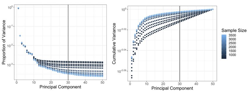
age in R. We found that 30 eigenvalues were sufficient to capture the most important features of the data and obtained
a very good prediction accuracy as shown in Fig. 3. Further studies omitted here found similar results as our 30 com-
ponents model for 50 and 100 eigenvectors. At the end of this operation, the reduced-order training set is now a matrix
X of size n × 30, and the reduced-order testing set is now a matrix X∗ of size m × 30.
Fig. 3: Proportion (left) and cumulative distribution (right) of variance in first 50 approximate principal components
in a simulation iteration. For all tested sample sizes the cumulative variance explained in the first 30 components is
more that 98% of that contained in the first 50 components.
3.2 2-Class Gaussian Process Classification
GPs are flexible, nonparametric Bayesian models that specify a prior distribution over a function f : X → Y that can
be updated by data D ⊂ X × Y [23]. Coarsely, a GP is a collection of random variables, any finite subset of whichhas a multivariate Gaussian distribution. We say that f ∼ G P(0, k(·, ·)), where k : X × X → R is a kernel: a positive
definite covariance function with hyperparameters θ .
We will model the function f mapping images embedded as described in subsection 3.1 to the scalar reals. Thus,
X = R30 is the input domain, and Y = R. In particular, we will discriminate between stars and galaxies on the basis
of whether our predicted evaluation of f is positive or negative. We will further assume that evaluations of f are
corrupted by noise introduced by the observation and preprocessing of data.
The Bayesian model for the GP prior on f for any finite X = {x1 , . . . , xn } ⊂ X is given by
y = f+ε (2)
>
f = [ f (x1 ), . . . , f (xn )] ∼ N (0, Kff ) (3)
ε ∼ N (0, σ I).2
(4)
Here y is an n-vector of the evaluations of f on X. N (µ, Σ) denotes the multivariate Gaussian distribution with
mean vector µ and covariance Σ. Kff is an n × n matrix whose (i, j)th element is k(xi , x j ) = cov( f (xi ), f (x j )). ε is
homoscedastic Gaussian noise affecting the measurement of f . Such covariance matrices implicitly depend on θ .
Say that we are given labelled data X, y ⊂ D. Here X is the set of n PCA-embedded images as described in subsec-
tion 3.1, and y is a conforming vector whose entries are +1 if the image has been deemed a star, and −1 otherwise.
Now consider the m unlabelled embedded images X∗ = {x∗1 , . . . , x∗m } ⊂ X . The joint distribution of y and the response
f∗ of f applied to X∗ is
K + σ 2 I Kf∗
y
= N 0, ff . (5)
f∗ K∗f K∗∗
Here K∗f = Kf∗> is the cross-covariance matrix between X and X, i.e. the (i, j)th element of K is k(x∗ , x ). Meanwhile,
∗ ∗f i j
K∗∗ has (i, j)th element k(x∗i , x∗j ). Applying Bayes rule to (3) and (5) allows us to analytically compute the posterior
distribution of the response f∗ on X∗ as
f∗ | X, X∗ , y ∼ N (f̄∗ ,C) (6)
f̄∗ ≡ K∗f Q−1
ff y (7)
C ≡ K∗∗ − K∗f Q−1
ff Kf∗ (8)
2
Qff ≡ Kff + σ I. (9)
We use a simple discriminator on the posterior of the response on X∗ : if f̄∗i ≥ 0, xi∗ is declared a star, and a galaxy
otherwise. Conveniently, we can examine the ith diagonal entry of C to quantify the variance of this prediction. This
allows us to automatically detect when the posterior variance is large, and the model is not confident in its prediction.
In this paper, we use the Radial Basis Function (RBF) kernel which is a very common choice for a wide range of
applications. It is expressed as:
kx − x0 k22
0
kRBF (x, x ) = exp − , (10)
`2
where the only hyperparameter ` is the length scale of the kernel. Hyperparameter estimation of ` is achieved by
maximizing prediction accuracy through local leave-one-out cross validation. σ 2 is fixed at the nominal value of
0.015.
4. RESULTS
Our main result is the vast performance increase, both in terms of accuracy and computing time, when working with a
reduced-order training data set vs the full-dimensional one. Fig. 4 shows that, unsurprisingly given the almost 800-fold
reduction in dimensionality, processing time is much lower and scales much better after a PCA reduction, and perhaps
more surprisingly, that the prediction accuracy also increases substantially. In particular, over the training sample
sizes tested, there is not a significant pattern of increasing mean accuracy with increased training size in the naive
method. In contrast, the mean accuracy of our method with data reduction performs better with 200 observations thanthe naive method with 2000 observations, and further improves as the training size increases. In terms of computing time, including an approximate PCA computation, with a training size of 2000, we reduce the computing time by approximately 86.4%. These results can be seen in Fig. 4. Fig. 4: Comparison of prediction accuracy and computing time as a function of training sample size with (black) and without (red). Reducing the dimensionality of the model before applying Gaussian Processes yields a better prediction accuracy and scales much better as the training sample size increases. We also explored the accuracy improvement of our methods for larger data sizes in Fig. 5. We see the mean accuracy improves when the number of training samples increases, but this increase is small when once the training sample size reaches 5000 (0.003 change for increase in training size from 5000 to 8000). At 5000 training samples, the accuracy is 0.96 and the processing time is about 15 seconds. Fig. 5: Prediction accuracy and computing time as a function of training sample size for the RBF kernel for large training sample sizes. The shaded region is the empirical simulation 94% prediction interval of performance. The prediction accuracy starts plateauing after 5000 samples and reaches a maximum accuracy of 0.96.
5.    CONCLUSION

We have shown that coupling a simple GP with an RBF kernel with a dimension-reducing embedding using ap-
proximate PCA drastically improves the prediction accuracy and computational efficiency of performing star-galaxy
separation. Not only does computational overhead grow more slowly with increasing data scale, but also our predic-
tion accuracy is higher with fewer training examples. By contrast, DNNs are highly parametric, often utilizing more
parameters than observations. For this reason, DNNs often require large amounts of training data whereas the present
method, which also has the advantage of providing full posterior distributions, is effective with only a modest amount
of labelled data.
In this paper we chose to use the RBF kernel as it is a common choice in the literature for many applications. However,
the expressiveness of a GP is heavily dependent upon the choice of kernel function. We suspect that significantly
improved accuracy is possible by utilizing more expressive kernel functions. Furthermore, we have yet to exploit the
GP posterior distributions to perform uncertainty quantification in this application. These investigations are to be the
subjects of future work.

                                             ACKNOWLEDGMENTS

This work was performed under the auspices of the U.S. Department of Energy by Lawrence Livermore National
Laboratory under Contract DE-AC52-07NA27344. Funding for this work was provided by LLNL Laboratory Directed
Research and Development grant 19-SI-004.

                                                      REFERENCES

 [1] T. M. C. Abbott, F. B. Abdalla, S. Allam, A. Amara, J. Annis, J. Asorey, S. Avila, O. Ballester, M. Banerji,
     W. Barkhouse, L. Baruah, M. Baumer, K. Bechtol, M. R. Becker, A. Benoit-Lévy, G. M. Bernstein, E. Bertin,
     J. Blazek, S. Bocquet, D. Brooks, D. Brout, E. Buckley-Geer, D. L. Burke, V. Busti, R. Campisano, L. Cardiel-
     Sas, A. Carnero Rosell, M. Carrasco Kind, J. Carretero, F. J. Castander, R. Cawthon, C. Chang, X. Chen,
     C. Conselice, G. Costa, M. Crocce, C. E. Cunha, C. B. D’Andrea, L. N. da Costa, R. Das, G. Daues, T. M.
     Davis, C. Davis, J. De Vicente, D. L. DePoy, J. DeRose, S. Desai, H. T. Diehl, J. P. Dietrich, S. Dodelson,
     P. Doel, A. Drlica-Wagner, T. F. Eifler, A. E. Elliott, A. E. Evrard, A. Farahi, A. Fausti Neto, E. Fernandez,
     D. A. Finley, B. Flaugher, R. J. Foley, P. Fosalba, D. N. Friedel, J. Frieman, J. Garcı́a-Bellido, E. Gaztanaga,
     D. W. Gerdes, T. Giannantonio, M. S. S. Gill, K. Glazebrook, D. A. Goldstein, M. Gower, D. Gruen, R. A.
     Gruendl, J. Gschwend, R. R. Gupta, G. Gutierrez, S. Hamilton, W. G. Hartley, S. R. Hinton, J. M. Hislop,
     D. Hollowood, K. Honscheid, B. Hoyle, D. Huterer, B. Jain, D. J. James, T. Jeltema, M. W. G. Johnson, M. D.
     Johnson, T. Kacprzak, S. Kent, G. Khullar, M. Klein, A. Kovacs, A. M. G. Koziol, E. Krause, A. Kremin, R. Kron,
     K. Kuehn, S. Kuhlmann, N. Kuropatkin, O. Lahav, J. Lasker, T. S. Li, R. T. Li, A. R. Liddle, M. Lima, H. Lin,
     P. López-Reyes, N. MacCrann, M. A. G. Maia, J. D. Maloney, M. Manera, M. March, J. Marriner, J. L. Marshall,
     P. Martini, T. McClintock, T. McKay, R. G. McMahon, P. Melchior, F. Menanteau, C. J. Miller, R. Miquel, J. J.
     Mohr, E. Morganson, J. Mould, E. Neilsen, R. C. Nichol, F. Nogueira, B. Nord, P. Nugent, L. Nunes, R. L. C.
     Ogand o, L. Old, A. B. Pace, A. Palmese, F. Paz-Chinchón, H. V. Peiris, W. J. Percival, D. Petravick, A. A.
     Plazas, J. Poh, C. Pond, A. Porredon, A. Pujol, A. Refregier, K. Reil, P. M. Ricker, R. P. Rollins, A. K. Romer,
     A. Roodman, P. Rooney, A. J. Ross, E. S. Rykoff, M. Sako, M. L. Sanchez, E. Sanchez, B. Santiago, A. Saro,
     V. Scarpine, D. Scolnic, S. Serrano, I. Sevilla-Noarbe, E. Sheldon, N. Shipp, M. L. Silveira, M. Smith, R. C.
     Smith, J. A. Smith, M. Soares-Santos, F. Sobreira, J. Song, A. Stebbins, E. Suchyta, M. Sullivan, M. E. C. Swan-
     son, G. Tarle, J. Thaler, D. Thomas, R. C. Thomas, M. A. Troxel, D. L. Tucker, V. Vikram, A. K. Vivas, A. R.
     Walker, R. H. Wechsler, J. Weller, W. Wester, R. C. Wolf, H. Wu, B. Yanny, A. Zenteno, Y. Zhang, J. Zuntz,
     DES Collaboration, S. Juneau, M. Fitzpatrick, R. Nikutta, D. Nidever, K. Olsen, A. Scott, and NOAO Data Lab.
     The Dark Energy Survey: Data Release 1. The Astrophysical Journal Supplement Series, 239(2):18, December
     2018. doi: 10.3847/1538-4365/aae9f0.
 [2] Hiroaki Aihara, Robert Armstrong, Steven Bickerton, James Bosch, Jean Coupon, Hisanori Furusawa, Yusuke
     Hayashi, Hiroyuki Ikeda, Yukiko Kamata, Hiroshi Karoji, Satoshi Kawanomoto, Michitaro Koike, Yutaka
Komiyama, Dustin Lang, Robert H Lupton, Sogo Mineo, Hironao Miyatake, Satoshi Miyazaki, Tomoki Mo-
rokuma, Yoshiyuki Obuchi, Yukie Oishi, Yuki Okura, Paul A Price, Tadafumi Takata, Manobu M Tanaka,
Masayuki Tanaka, Yoko Tanaka, Tomohisa Uchida, Fumihiro Uraguchi, Yousuke Utsumi, Shiang-Yu Wang,
Yoshihiko Yamada, Hitomi Yamanoi, Naoki Yasuda, Nobuo Arimoto, Masashi Chiba, Francois Finet, Hiroki
Fujimori, Seiji Fujimoto, Junko Furusawa, Tomotsugu Goto, Andy Goulding, James E Gunn, Yuichi Harikane,
Takashi Hattori, Masao Hayashi, Krzysztof G Hełminiak, Ryo Higuchi, Chiaki Hikage, Paul T P Ho, Bau-
Ching Hsieh, Kuiyun Huang, Song Huang, Masatoshi Imanishi, Ikuru Iwata, Anton T Jaelani, Hung-Yu Jian,
Nobunari Kashikawa, Nobuhiko Katayama, Takashi Kojima, Akira Konno, Shintaro Koshida, Haruka Kusak-
abe, Alexie Leauthaud, Chien-Hsiu Lee, Lihwai Lin, Yen-Ting Lin, Rachel Mandelbaum, Yoshiki Matsuoka,
Elinor Medezinski, Shoken Miyama, Rieko Momose, Anupreeta More, Surhud More, Shiro Mukae, Ryoma
Murata, Hitoshi Murayama, Tohru Nagao, Fumiaki Nakata, Mana Niida, Hiroko Niikura, Atsushi J Nishizawa,
Masamune Oguri, Nobuhiro Okabe, Yoshiaki Ono, Masato Onodera, Masafusa Onoue, Masami Ouchi, Tae-Soo
Pyo, Takatoshi Shibuya, Kazuhiro Shimasaku, Melanie Simet, Joshua Speagle, David N Spergel, Michael A
Strauss, Yuma Sugahara, Naoshi Sugiyama, Yasushi Suto, Nao Suzuki, Philip J Tait, Masahiro Takada, Tsuyoshi
Terai, Yoshiki Toba, Edwin L Turner, Hisakazu Uchiyama, Keiichi Umetsu, Yuji Urata, Tomonori Usuda, Sherry
Yeh, and Suraphong Yuma. First data release of the Hyper Suprime-Cam Subaru Strategic Program. Publica-
tions of the Astronomical Society of Japan, 70(SP1), 10 2017. ISSN 0004-6264. doi: 10.1093/pasj/psx081. URL
https://doi.org/10.1093/pasj/psx081. S8.
[3] James Baglama and Lothar Reichel. Augmented implicitly restarted lanczos bidiagonalization methods. SIAM
Journal on Scientific Computing, 27(1):19–42, 2005.
[4] Charles Blundell, Julien Cornebise, Koray Kavukcuoglu, and Daan Wierstra. Weight uncertainty in neural net-
works. arXiv preprint arXiv:1505.05424, 2015.
[5] James Bosch, Robert Armstrong, Steven Bickerton, Hisanori Furusawa, Hiroyuki Ikeda, Michitaro Koike, Robert
Lupton, Sogo Mineo, Paul Price, Tadafumi Takata, et al. The hyper suprime-cam software pipeline. Publications
of the Astronomical Society of Japan, 70(SP1):S5, 2018.
[6] John Bradshaw, Alexander G de G Matthews, and Zoubin Ghahramani. Adversarial examples, uncertainty, and
transfer testing robustness in gaussian process hybrid deep networks. arXiv preprint arXiv:1707.02476, 2017.
[7] Ross Fadely, David W Hogg, and Beth Willman. Star-galaxy classification in multi-band optical imaging. The
Astrophysical Journal, 760(1):15, 2012.
[8] Yarin Gal and Zoubin Ghahramani. Dropout as a bayesian approximation: Representing model uncertainty in
deep learning. In international conference on machine learning, pages 1050–1059, 2016.
[9] Chuan Guo, Geoff Pleiss, Yu Sun, and Kilian Q Weinberger. On calibration of modern neural networks. arXiv
preprint arXiv:1706.04599, 2017.
[10] Edward J Kim and Robert J Brunner. Star-galaxy classification using deep convolutional neural networks.
Monthly Notices of the Royal Astronomical Society, page stw2672, 2016.
[11] Edward J Kim, Robert J Brunner, and Matias Carrasco Kind. A hybrid ensemble learning approach to star–galaxy
classification. Monthly Notices of the Royal Astronomical Society, 453(1):507–521, 2015.
[12] Alex Krizhevsky, Ilya Sutskever, and Geoffrey E Hinton. Imagenet classification with deep convolutional neural
networks. In Advances in neural information processing systems, pages 1097–1105, 2012.
[13] Alexie Leauthaud, Richard Massey, Jean-Paul Kneib, Jason Rhodes, David E. Johnston, Peter Capak, Cather-
ine Heymans, Richard S. Ellis, Anton M. Koekemoer, Oliver Le Fèvre, Yannick Mellier, Alexandre Réfrégier,
Annie C. Robin, Nick Scoville, Lidia Tasca, James E. Taylor, and Ludovic Van Waerbeke. Weak Gravitational
Lensing with COSMOS: Galaxy Selection and Shape Measurements. The Astrophysical Journal Supplement
Series, 172(1):219–238, September 2007. doi: 10.1086/516598.
[14] Satoshi Miyazaki, Yutaka Komiyama, Satoshi Kawanomoto, Yoshiyuki Doi, Hisanori Furusawa, Takashi
Hamana, Yusuke Hayashi, Hiroyuki Ikeda, Yukiko Kamata, Hiroshi Karoji, Michitaro Koike, Tomio Kurakami,Shoken Miyama, Tomoki Morokuma, Fumiaki Nakata, Kazuhito Namikawa, Hidehiko Nakaya, Kyoji Nariai,
Yoshiyuki Obuchi, Yukie Oishi, Norio Okada, Yuki Okura, Philip Tait, Tadafumi Takata, Yoko Tanaka, Masayuki
Tanaka, Tsuyoshi Terai, Daigo Tomono, Fumihiro Uraguchi, Tomonori Usuda, Yousuke Utsumi, Yoshihiko Ya-
mada, Hitomi Yamanoi, Hiroaki Aihara, Hiroki Fujimori, Sogo Mineo, Hironao Miyatake, Masamune Oguri, To-
mohisa Uchida, Manobu M. Tanaka, Naoki Yasuda, Masahiro Takada, Hitoshi Murayama, Atsushi J. Nishizawa,
Naoshi Sugiyama, Masashi Chiba, Toshifumi Futamase, Shiang-Yu Wang, Hsin-Yo Chen, Paul T. P. Ho, Eric
J. Y. Liaw, Chi-Fang Chiu, Cheng-Lin Ho, Tsang-Chih Lai, Yao-Cheng Lee, Dun-Zen Jeng, Satoru Iwamura,
Robert Armstrong, Steve Bickerton, James Bosch, James E. Gunn, Robert H. Lupton, Craig Loomis, Paul Price,
Steward Smith, Michael A. Strauss, Edwin L. Turner, Hisanori Suzuki, Yasuhito Miyazaki, Masaharu Mura-
matsu, Koei Yamamoto, Makoto Endo, Yutaka Ezaki, Noboru Ito, Noboru Kawaguchi, Satoshi Sofuku, Tomoaki
Taniike, Kotaro Akutsu, Naoto Dojo, Kazuyuki Kasumi, Toru Matsuda, Kohei Imoto, Yoshinori Miwa, Masayuki
Suzuki, Kunio Takeshi, and Hideo Yokota. Hyper Suprime-Cam: System design and verification of image qual-
ity. Publications of the Astronomical Society of Japan, 70:S1, January 2018. doi: 10.1093/pasj/psx063.
[15] S. C. Odewahn, E. B. Stockwell, R. L. Pennington, R. M. Humphreys, and W. A. Zumach. Automated star/galaxy
discrimination with neural networks. In H. T. MacGillivray and E. B. Thomson, editors, Digitised Optical Sky
Surveys, pages 215–224, Dordrecht, 1992. Springer Netherlands. ISBN 978-94-011-2472-0.
[16] SC Odewahn, EB Stockwell, RL Pennington, Roberta M Humphreys, and WA Zumach. Automated star/galaxy
discrimination with neural networks. In Digitised Optical Sky Surveys, pages 215–224. Springer, 1992.
[17] Pollo, A., Rybka, P., and Takeuchi, T. T. Star-galaxy separation by far-infrared color-color diagrams for the akari
fis all-sky survey (bright source catalog version β−1). A&A, 514:A3, 2010. doi: 10.1051/0004-6361/200913428.
URL https://doi.org/10.1051/0004-6361/200913428.
[18] Ignacio Sevilla-Noarbe and Penélope Etayo-Sotos. Effect of training characteristics on object classification: An
application using boosted decision trees. Astronomy and Computing, 11:64–72, 2015.
[19] Colin T. Slater, Željko Ivezić, and Robert H. Lupton. Morphological star–galaxy separation. The Astronom-
ical Journal, 159(2):65, jan 2020. doi: 10.3847/1538-3881/ab6166. URL https://doi.org/10.3847/
1538-3881/ab6166.
[20] The Dark Energy Survey Collaboration. The Dark Energy Survey. arXiv e-prints, art. astro-ph/0510346, October
2005.
[21] E. C. Vasconcellos, R. R. de Carvalho, R. R. Gal, F. L. LaBarbera, H. V. Capelato, H. Frago Campos Velho,
M. Trevisan, and R. S. R. Ruiz. Decision tree classifiers for star/galaxy separation. The Astronomical Journal,
141(6):189, may 2011. doi: 10.1088/0004-6256/141/6/189. URL https://doi.org/10.1088/0004-6256/
141/6/189.
[22] EC Vasconcellos, RR De Carvalho, RR Gal, FL LaBarbera, HV Capelato, H Frago Campos Velho, Marina
Trevisan, and RSR Ruiz. Decision tree classifiers for star/galaxy separation. The Astronomical Journal, 141(6):
189, 2011.
[23] Christopher KI Williams and Carl Edward Rasmussen. Gaussian processes for machine learning. MIT press
Cambridge, MA, 2006.You can also read