Evolution Model of Spatial Interaction Network in Online Social Networking Services - MDPI
←
→
Page content transcription
If your browser does not render page correctly, please read the page content below
entropy
Article
Evolution Model of Spatial Interaction Network in
Online Social Networking Services
Jian Dong 1 , Bin Chen 1, * , Pengfei Zhang 1 , Chuan Ai 1 , Fang Zhang 1 , Danhuai Guo 2,3
and Xiaogang Qiu 1
 1   College of System Engineering, National University of Defense Technology, Changsha 410073, China;
     jiandong.nudt@foxmail.com (J.D.); hncszpf@163.com (P.Z.); rogeraichuan@gmail.com (C.A.);
     fangzhang.nudt@foxmail.com (F.Z.); 13874934509@139.com (X.Q.)
 2   Computer Network Information Center, Chinese Academy of Sciences,
     4th South Fourth Road Zhongguancun, Beijing 100190, China; guodanhuai@cnic.cn
 3   University of Chinese Academy of Sciences, 19th Yuquan Road, Beijing 100049, China
 *   Correspondence: nudtcb9372@gmail.com; Tel.: +86-0731-8457-4332

 Received: 22 March 2019; Accepted: 23 April 2019; Published: 24 April 2019

 Abstract: The development of online social networking services provides a rich source of data of social
 networks including geospatial information. More and more research has shown that geographical
 space is an important factor in the interactions of users in social networks. In this paper, we construct
 the spatial interaction network from the city level, which is called the city interaction network, and
 study the evolution mechanism of the city interaction network formed in the process of information
 dissemination in social networks. A network evolution model for interactions among cities is
 established. The evolution model consists of two core processes: the edge arrival and the preferential
 attachment of the edge. The edge arrival model arranges the arrival time of each edge; the model of
 preferential attachment of the edge determines the source node and the target node of each arriving
 edge. Six preferential attachment models (Random-Random, Random-Degree, Degree-Random,
 Geographical distance, Degree-Degree, Degree-Degree-Geographical distance) are built, and the
 maximum likelihood approach is used to do the comparison. We find that the degree of the node and
 the geographic distance of the edge are the key factors affecting the evolution of the city interaction
 network. Finally, the evolution experiments using the optimal model DDG are conducted, and the
 experiment results are compared with the real city interaction network extracted from the information
 dissemination data of the WeChat web page. The results indicate that the model can not only capture
 the attributes of the real city interaction network, but also reflect the actual characteristics of the
 interactions among cities.

 Keywords: city interaction network; evolution model; preferential attachment; WeChat; maximum
 likelihood

1. Introduction
     With the rapid development of the Internet, smart phones, and information technology, online
social networking services such as Facebook, Twitter, Sina Weibo, and WeChat have developed rapidly.
These platforms facilitate the interactions among users and accelerate the dissemination of emotions
and opinions contained in the information. Meanwhile, these platforms provide a rich source of social
media including geospatial information for the research of social networks [1–4]. The interactions of
users in social networks usually manifest as the viewing and forwarding of information. More and
more research shows that geographical space, which seems to be a bridge between online and offline,
affects the interactions of users in social networks [5–7].

Entropy 2019, 21, 434; doi:10.3390/e21040434                                  www.mdpi.com/journal/entropy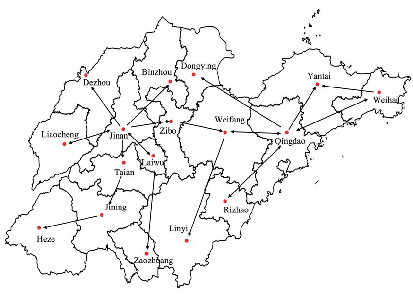
Entropy 2019, 21, 434                                                                                2 of 17

      Spatial interaction is the process whereby entities at different points in physical space make
contacts, demand/supply decisions, or locational choices [8]; for example, trade in goods among
different countries or regions, human migration among cities or countries, and people in different
cities communicating with each other by phone or social media software. In social networks, spatial
interactions are formed by users who belong to different spatial locations through viewing and
forwarding information. Naturally, spatial interactions can be described by complex network [9],
where nodes represent spatial locations, which can be cities, provinces, or countries, and edges
represent interactions of entities in different spatial locations. The research on the characteristics
of the spatial interaction network in social networks and their evolutionary mechanisms is of great
significance for providing location-based business services, planning and managing communication
network facilities, and formulating regional economic development policies. In addition, the results
also can be used to improve the performances of several types of applications in various fields, such as
social network analysis [10] and affective computing [11–13].
      The existing network evolution models mainly include the random graph models
(RGM) [14–16], generated network models (GNM) [17,18], and data-driven network models
(DDNM) [19–21]. Random graph models, such as Poisson random graphs and generalized random
graphs, attempt to apply the connecting probability and changing strategy of the edge to a certain
number of nodes to generate a random network that meets specific statistical characteristics (such
as average degree, degree distribution, joint degree distribution, and degree-degree correlation).
Generated network models, such as preferential attachment models and their variants, try to generate
a network that reflects certain characteristics of the real network (such as a power-law distribution,
small-world characteristics, and homogeneity) through certain node-adding, edge-adding, and
edge-changing rules from simple graphs (regular graphs). These two widely-used models can
usually generate networks with some characteristics of the real network, but they cannot satisfy
multiple characteristics at the same time. Moreover, these models usually do not consider the
geospatial characteristics of networks, making it difficult to describe the evolution process of spatial
interaction network.
      Generally, distance and location are the two important factors of geospatial characteristics. On the
one hand, it is found that the interaction frequency among users has a distance decay effect. People
tend to communicate more with friends who are close to them geographically, while users who are far
away from each other are less likely to interact [22–25]. On the other hand, the behaviors of people
living in similar geographical locations, such as the same city, often show similarities, while people in
different geographical locations will have different behavior patterns due to economic and cultural
differences, thus affecting the information interactions among regions [22].
      Gravity laws are commonly found in spatial interaction networks such as crowd flow networks,
population migration networks, and commodity trade networks. Thus, a gravity model for spatial
interaction is proposed by analogy with the law of universal gravitation. The gravity model provides
an estimate of the traffic between two or more regions (such as the number of trips and the quantity
of commodity trade). In a spatial interaction network, the gravity model can be interpreted as the
frequency of interactions between two nodes. The frequency is proportional to the strength of the two
nodes and inversely proportional to the power of the distance between the two nodes. The gravity
model has become a classic model for interpreting and predicting the interactions of spatial networks
and is widely used in many fields including transportation planning [26], population migration [27,28],
international trade [29,30], and disease transmission [31]. Although the gravity model is simple,
intuitive, easy to calculate, and involves geographical factors, it lacks a rigorous theoretical foundation.
In addition, the gravity model is deterministic and cannot explain the fluctuation of the interaction
between two nodes in the spatial interaction network [32]. Therefore, this kind of static estimation is
not suitable for describing the evolution of spatial networks.
      This paper proposes a spatial interaction network at the city level, which is called the city
interaction network. We study the evolution mechanism of the city interaction network formed
Entropy 2019, 21, 434 3 of 17
in the process of information dissemination in social networks, where nodes represent cities and
edges represent interactions among cities. We consider the evolution model of the city interaction
network from the perspective of the edge, that is how each edge is added to the city interaction
network. A evolution model for describing the interactions among cities is established. The
evolution model consists of two core processes: the edge arrival and the preferential attachment
of the edge. The edge arrival model arranges the arrival time of each edge; the model of preferential
attachment of the edge determines the source node and the target node of each arriving edge. Six
preferential attachment models (Random-Random, Random-Degree, Degree-Random, Geographical
distance, Degree-Degree, Degree-Degree-Geographical distance) are built, and the maximum likelihood
approach is used to do the comparison. Finally, the evolution experiments using the optimal model
(Degree-Degree-Geographical distance) are conducted, and the experiment results are compared with
the real city interaction network extracted from the information dissemination data of the WeChat
web page.
Preferential attachment of edges: The preferential attachment model assumes that when a new
node joins the network, it creates a constant number of edges, where the selection of the target node
for each edge is proportional to the degree of the node [33]. In addition to degree, the node age and
geographic distance of the edge can be applied to the preferential attachment model [34]. This paper
considers the evolution of the network from the perspective of the edge. Therefore, when an edge
is added to the network, the source node and the target node are selected according to preferential
attachment of edges.
Evaluation by the maximum likelihood: The maximum likelihood approach is usually used to
compare a series of models numerically and select the best model (and parameters) to interpret the
data [35]. As our understanding of real-world networks improves, likelihood remains unchanged,
while the generative models improve to incorporate the new understanding. Success in modeling can
therefore be effectively tracked [34]. The maximum likelihood approach is widely used to estimate
network model parameters [35–37] and select the optional model [34,38]. Therefore, this paper uses
the maximum likelihood approach to evaluate and compare different network evolution models based
on empirical data.
WeChat: WeChat is one of the most popular social networking platforms in China. As of the
second quarter of 2016, WeChat has covered more than 94% smart phones in China, with 0.8 billion
monthly active users. WeChat has powerful social functions and a large number of users, and
WeChat has integrated almost all aspects of people’s lives, including payment, location-based services,
shopping, games, and entertainment. Therefore, WeChat is an appropriate system to study the
characteristics and evolution mechanism of the spatial interaction network in social networks.
The rest of this paper is organized as follows: the second section introduces the dissemination
data of the WeChat web page and constructs the city interaction network. The third section introduces
the evolution model of the city interaction network. In the fourth section, the maximum likelihood
method is used to evaluate the six preferential attachment models and to select the optimal model and
parameters. In the fifth section, the optimal model is used for network evolution, and the obtained
evolutionary network is compared with the real city interaction network. The potential biases and
model extension are discussed in the sixth section, and the seventh section is the conclusion.
2. Preliminaries
2.1. Dataset
WeChat provides three basic functions: instant messaging (including single and group chat),
moments (where users publish, comment, and forward information), and official accounts (including
subscription accounts and service accounts). Users can interact with their friends by posting text,
voice, pictures, emoticons, location, video, web links, and other information. This paper studies the
dissemination data of the WeChat web page (HTML5) collected by third-party service companies.Entropy 2019, 21, 434 4 of 17
The recording process of the WeChat web page data can be described as: when a web page with a
certain theme is created and published by the creator through the official accounts, the content of this
web page can be viewed by other users. Users who view the web page can send it to their moments
or WeChat friends, or not forward it. Thus, the users who view (or forward) and the users who are
viewed (or forwarded) are recorded.
The dissemination data of WeChat web page were obtained, and the time span of the data was
from 2–8 July 2016. There were 622,637 records in total, and each record can be represented by a
six-tuple , where pageID represents the unique identity
of the web page, sourceID and targetID represent the unique identity of the user, type represents the
behavior type of target, including viewing and forwarding, time represents the time when the behavior
of targetID occurs, and ip represents the IP address of targetID. In order to protect the privacy of users,
web page identity and user identity were anonymized.
2.2. City Interaction Network
Most of the researches related to geography use self-reported data to identify the location of
users, which is often inaccurate. By locating users with IP addresses, the errors of self-reported data
can be avoided. Song et al. analyzed several large IP address databases, including the Chunzhen
IP address database, the Taobao IP address database, the Sina IP address database, and the Baidu
IP address database [39]. They found that the four IP address databases were quite different, and
when the administrative division level was lower, the coverage rate and coincidence rate of IP address
databases would decrease, while the data availability would also decrease. However, considering the
coverage rate and coincidence rate of the four IP address databases, they believed that the credibility
of the Taobao IP database was the highest. Therefore, the Taobao IP address database was used in our
work to locate the IP address in the data to the corresponding cities in China. Finally, the IP address
in the data was located in 34 provincial divisions of China (including 23 provinces, 4 municipalities,
5 autonomous regions, and 2 special administrative regions), a total of 372 cities. The number of cities
corresponding to each provincial division is shown in Table 1.
Table 1. City distribution of 34 provincial divisions in China. China has 34 provincial divisions,
including 23 provinces, 4 municipalities, 5 autonomous regions, and 2 special administrative regions.
Province Number of Cities Province Number of Cities Province Number of Cities
Beijing 1 Tianjin 1 Hebei 11
Inner Mongolia 12 Liaoning 14 Jilin 9
Shanghai 1 Jiangsu 13 Zhejiang 21
Fujian 16 Jiangxi 9 Shandong 11
Hubei 18 Hunan 17 Guangdong 14
Hainan 18 Chongqing 1 Sichuan 21
Yunnan 16 Xizang 7 Shannxi 10
Qinghai 8 Ningxia 5 Xinjiang 15
Shanxi 11 Heilongjiang 13 Anhui 11
Henan 17 Guangxi 14 Guizhou 9
Gansu 14 Hong Kong 1 Macao 1
Taiwan 12
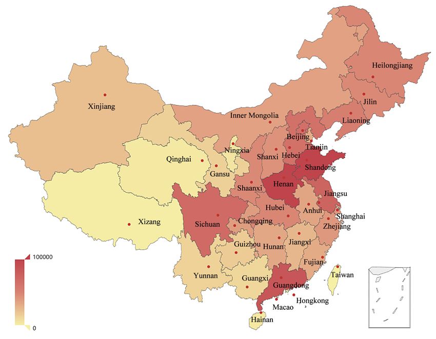
Figure 1 shows the active frequency of users in each provincial division. The active frequency of a
province is the number of users located in that province. The active frequency was more in the east
and less in the west. The top three provincial divisions with the highest frequency were Shandong,
Henan, and Guangdong, and the active frequency of Xizang, Xinjiang, and Taiwan was low. This
fully reflects that information interaction is affected by political, economic, cultural, geographical, and
demographic factors.Entropy 2019, 21, 434 5 of 17
Figure 1. The active frequency of users in 34 provincial divisions of China. The transition of colors
from red to yellow indicates the reduction of active frequency, and the corresponding data of each color
are given by the color bar in the lower left corner.
Based on the data of the web page dissemination in WeChat, the city interaction network Gt =
(V, Et , Wt ) can be constructed. Gt is a dynamic directed network, V = {v1 , v2 , v3 , · · · , v N } is the
set of nodes in the network, representing cities of China, and the number of nodes is N; Et =
{e1 , e2 , e3 , · · · , e Mt } is the set of edges of the network from Time 0–t, representing the interactions
among cities, and the number of edges is Mt ; Wt = {w1 , w2 , w3 , · · · , w Mt } is the weight set of edges in
the network from Time 0–t, representing the number of interactions among cities. The dynamics of the
city interaction network Gt is reflected in the changes of the edge and weight. We took the cities in
Shandong province as an example to elaborate the construction process of the city interaction network.
At t = 0, Gt is a network containing only 17 isolated nodes (the number of cities in Shandong province).
When a WeChat web page is published by a user in Jinan and users in Dezhou view or forward this
web page, then a directed edge from Jinan to Dezhou is established. The weight of the directed edge is
the number of Dezhou users viewing the web page. With the dissemination of the web page, it was
assumed that the interaction network one day later is as shown in Figure 2. At this time, the number
of nodes in the interaction network was N = 17, and the number of edges was Mt = 22 (bidirectional
edges are denoted as two edges), where t = 1 (day). The city interaction network in this paper allows
self-connected edges, which represents the interactions in the same city.Entropy 2019, 21, 434 6 of 17
Figure 2. Schematic diagram of the city interaction network in Shandong province. Red dots represent
the nodes of the network, and black arrows represent the directed edges of the network. The arrows
start from the source node and point to the target node. The bidirectional arrow indicates that the two
nodes are source and target nodes of each other.
Take the starting time of data (2 July 2016 00:00) as the time t = 0, and construct the city interaction
network. The time span of the network is T. Table 2 lists the basic properties of the network GT ,
including the number of nodes, number of edges, number of self-connected edges, average degree of
nodes, density, average clustering coefficient, and average shortest path length.
Table 2. Basic properties of the city interaction network GT . N represents the number of nodes, MT the
avg
number of edges, MTse the number of self-connected edges, k T the average degree of nodes, ρ T the
density, and L T the average length of the shortest path.
avg
T N MT MTse kT ρT LT
2–8 July 2016 372 30,438 353 163.65 0.22 1.73
According to the basic properties of the network GT listed in Table 2, an overall understanding
of the interaction among cities was obtained through the dissemination of WeChat web page. The
network involved 372 nodes and 30,438 edges, which indicates that not every two nodes had connected
edges. On average, each node only had connections with 163.65 nodes, and the density of the network
was only 0.22. It can be seen that although WeChat has a large number of users in China and covers all
cities, each city will not interact with all other cities in the short term. The average shortest path length
of the network was 1.73, which means that the average hop from one node to another node was 1.73.
There were 353 self-connected edges in the network, and only 19 nodes had no self-connected edges. A
total of 622,637 interaction records were recorded, among which, 350,578 records were the interactions
in the same city, accounting for 56%. It can be seen that users were more inclined to interact with users
in the same city.
Figure 3 shows the number of non-isolated nodes and the number of edges in the city interaction
network as a function of time. Figure 3a shows the number of non-isolated nodes in the city interaction
network as a function of time. Non-isolated nodes represent the nodes that have interacted with other
nodes. In the initial stage, the number of non-isolated nodes grew rapidly, and the growth became slow
until the number of nodes was close to N. Figure 3b shows the number of edges in the city interactionEntropy 2019, 21, 434 7 of 17
network as a function of time. The number of edges in the network kept increasing, but due to the
limitation of the number of nodes, the growth of the number of edges gradually slowed down. In
the case where the number of non-isolated nodes in the network was almost constant, the number
of edges still kept growing. This also reflects the limitations of the evolution of the city interaction
network from the perspective of nodes.
× 104
400 3.5
350 3
300
2.5
non-isolated nodes
250
2
edges
200
1.5
150
1
100
50 0.5
0 0
0 50 100 150 200 0 50 100 150 200
time (hour) time (hour)
(a) (b)
Figure 3. The number of non-isolated nodes and the number of edges in the city interaction network as
a function of time. (a) The number of non-isolated nodes in the city interaction network as a function
of time. (b) The number of edges in the city interaction network as a function of time. Each data point
in the figure represents the number of non-isolated nodes (or edges) in the city interaction network
from t = 0 to the current time. The time interval between two data points is one hour.
2.3. Notation
Let Z denote the set of edges to be added to the network, t(z), z ∈ Z the time when an edge z
is added to the network, and ztu,v an edge z added to the network at time t, and its source node and
target node are connected to node u and node v respectively. Let k t (v) denote the degree of node v at
time t and d(u, v) denote the geography distance between node u and node v.
3. Evolution Model
We consider the evolution model of the city interaction network from the perspective of the edge.
The model consists of two core processes: the edge arrival and the preferential attachment of the edge.
The edge arrival determines the arrival time of each edge; the preferential attachment of the edge
determines the source node and the target node of each arriving edge.
For an edge z, it is composed of a node pair:
z = (u, v), u, v ∈ V, (1)
where V represents the node set and does not change with the network evolution. Assuming that the
arrival time of the edges is a function of time in ∆t, then the arrival time of each edge in ∆t will be
arranged, and all edges can be expressed in the time sequence according to the arrival time:
Z = z t1 , z t2 , · · · , z t C , (2)
t1 6 t2 6 · · · 6 t C , (3)Entropy 2019, 21, 434 8 of 17
where C is the length of the sequence Z, and Formula (3) guarantees the time-ordered arrival of
the edges.
Select the source node u and the target node v from node set V according to a certain preferential
attachment for the edge arriving at time t:
P(ztu,v ) ∼ X (Θ), (4)
where X (Θ) represents a distribution function and Θ is the parameter of the distribution function.
Finally, the network evolution is realized by updating the edge and weight. The edge arrival and
preferential attachment of the edge are described in detail below.
3.1. Edge Arrival
Figure 4 shows the interaction quantity among cities of the data (each record represents an
interaction) as a function of time. In the figure, each data point represents the interaction quantity
among cities from time t = 0 to the current time, and the red line is the fitting of the function. It can
be seen from the figure that the interaction quantity was a linear function of time, which satisfies
f (t) = 4025t − 4.51e4, and the time unit is hours. Since each edge represents the interaction among
nodes, f (t) can be used to describe the number of arriving edges. Thus, the number of edges added
to the network per unit time is a constant ε = 4025, and the time interval for each arriving edge is
ti − ti−1 = 1/ε, i = 2, 3, · · · , C. Let the time of the first arrived edge be t1 = 0, so that the time of each
arriving edge is determined.
× 105
8
f(t)=4025t-4.51e4
6
interactions
4
2
0
-2
0 50 100 150
time (h)
Figure 4. The interaction quantity among cities of the data as a function of time. Each data point
represents the interaction quantity among cities from time t = 0 to the current time, and the red line is
the fitting for the function; the fitting expression is given in the figure.
3.2. Preferential Attachment of the Edge
In this paper, the evolution of the city interaction network is considered from the perspective of
the edge. Therefore, when an edge is added to the network, its source node and the target node will be
selected according to a certain mechanism. This selection mechanism is called preferential attachment
of the edge. Here, six different preferential attachment models are considered in this paper:Entropy 2019, 21, 434 9 of 17
Random-Random (RR): for the arrived edge at time t, two nodes are randomly selected from the node
set V as its source node and the target node, respectively:
1
PRR (ztu,v ) = . (5)
Nt2
Random-Degree (RD): for the arriving edge at time t, a node is randomly selected from the node set
V as its source node, and the selection of its target node is proportional to the degree of nodes in
the network:
[k t (v)]α
PRD (ztu,v ) = . (6)
N ∑i∈V [k t (i )]α
Degree-Random (DR): for the arrived edge at time t, a node is randomly selected from the node set
V as its target node, and the selection of its source node is proportional to the degree of nodes in
the network:
[k t (u)] β
PDR (ztu,v ) = . (7)
N ∑i∈V [k t (i )] β
Geographical distance (G): for the arrived edge at time t, the selection of its source node and target
node is proportional to the geographical distance between the two nodes:
[d(u, v)]γ
PG (ztu,v ) = . (8)
∑i,j∈V [d(i, j)]γ
Degree-Degree (DD): for the arrived edge at time t, the selection of its source node and target node is
proportional to the degree of the nodes in the network. The degree index for the source node is α, and
the degree index for the target node is β:
[k t (v)]α [k t (u)] β
PDD (ztu,v ) = . (9)
∑i,j∈V [k t (i )]α [k t ( j)] β
Degree-Degree-Geographical distance (DDG): for the arrived edge at time t, the selection of its
source node and target node is proportional to the degree of the nodes in the network and to the
geographical distance between the source node and the target node. The degree index for the source
node is α; the degree index for the target node is β; and the distance index is γ:
[k t (v)]α [k t (u)] β [d(u, v)]γ
PDDG (ztu,v ) = . (10)
∑i,j∈V [k t (i )]α [k t ( j)] β [d(i, j)]γ
4. Evaluation
In this section, a quantitative approach is applied to compare the accuracies of different preferential
attachment models. The network is often considered to be the result of an evolutionary random
process that drives its growth, including new nodes and new edges [35]. Given real data about
network evolution, the extent to which the assumptions of a model are supported by the data using
the maximum likelihood approach can be tested. The maximum likelihood approach is usually used
to compare a series of models numerically and to select the best model (and parameters) to interpret
the data. Estimating the likelihood of a preferential attachment model M involves considering each
arriving edge zt and computing the likelihood PM (ztu,v ) that the edge zt selects the actual source node
u and the actual target node v according to the model M. Therefore, the likelihood of network GT
generated by model M can be expressed as:
PM ( GT ) = ∏ PM (ztu,v ). (11)
t∈ TEntropy 2019, 21, 434 10 of 17
To obtain better numerical accuracy, the log-likelihood is used in this paper:
log(∏ PM (ztu,v )) = ∑ log( PM (ztu,v )). (12)
t t
Since the city interaction network had self-connecting edges, which represents the interaction
in the same city, we assumed that the distance of self-connecting edges was 20 kilometers (consider
each city contour as a circle, and 20 kilometers is the approximate average of the radius of all cities).
Figure 5 shows the relationship between the log-likelihood of models and different parameters. The
RR model had no parameters, and its log-likelihood was a constant −3,185,899. In addition to the RR
model, the log-likelihoods of the other five models were all convex functions of the model parameters,
so the maximum likelihood of each model can be found to estimate the best parameters of the model.
Table 3 lists the maximum log-likelihood of different preferential attachment models and the optimal
parameters under the maximum log-likelihood. It can be seen from Figure 5 that, under the same
parameter, the log-likelihood of the RD model and DR model was approximately equal. This reflects
that the RD model and DR model had similar effects on the network evolution, and the selection of
the source node and the target node was equal. Figure 5d also reflects this point. Figure 5c shows the
relationship between the log-likelihood and parameter γ of G model, and its maximum log-likelihood
was significantly higher than that of the RR model, RD model, DR model, and DD model, indicating
that the distance played an important role in the evolution of the city interaction network. The DDG
model considered both the node degree and the geography distance among nodes in the network
evolution process. It can be seen that the maximum log-likelihood of DDG model was the highest,
which was 22% higher than that of the DD model and 11% higher than that of the G model. In addition,
in the DD model, when α = 1.0, β = 1.0, its log-likelihood was the maximum. In the G model, when
γ = −1.6, its log-likelihood was the maximum. The DDG model, which considered the node degree
and the geography distance, obtained the maximum likelihood when α = 0.6, β = 0.6, γ = −1.5. This
indicates that the distance made the degree of the node less important. Then, we applied the DDG
preferential attachment model with parameters α = 0.6, β = 0.6, γ = −1.5 to the evolution of the city
interaction network.
5. Network Evolution
In order to verify the city interaction network model and the evolution process of the network,
network evolution experiments were conducted. We considered the real network G3T/4 from 2–4 July
2016 and evolved it from t = 34 T until t = T. Specifically, the edge arrival model was used to determine
the edges arriving at time t ∈ [ 34 T, T ]. For each arriving edge, the DDG preferential attachment model
0
was used to select its source node and target node. Finally, the evolutionary network GT with the same
0
time length as the real network GT was obtained. GT and GT were analyzed by the comparison of the
statistical characteristics and community structure of the network.
0
Figure 6 shows the statistical characteristics of real network GT and evolutionary network GT .
Figure 6a,b are considered from the edge properties. Figure 6a shows the weight distribution of
the edges. It can be seen that the weight distributions of the real network and the evolutionary
network followed the power-law distribution. The weight distribution of real network GT was fitted as
shown in the dotted black line. The power exponents of the weight distributions of real network and
evolutionary network were 1.92 and 1.99, respectively (the weight distributions of the real network
and evolutionary network approximately overlapped, so the fit line of the weight distribution of
the evolutionary network is not drawn). The weight of the edge represents the interaction among
cities, and the power-law distribution of the weight distribution reflects that only a few cities had
frequent interactions, while the interactions among most cities was very small. Figure 6b shows the
geographical distance distribution of edges. The geographical distance distribution of edges is a
property that connects the network with geographical space. Most of the interactive distances among
cities were about 100 km. As the distance continued to increase, the probability of interaction becameEntropy 2019, 21, 434 11 of 17
smaller. In addition, 20 km was also the high-frequency distance of city interaction (the distance was
denoted as 20 km if the interaction occurred in the same city), indicating that the interaction in the
same city occupied a large proportion.
× 106 × 106 × 106
-2.95 -2.95 -2.4
-2.5
-3 -3 -2.6
-2.7
log likehood
log likehood
log likehood
-3.05 -3.05
-2.8
-2.9
-3.1 -3.1
-3
-3.15 -3.15 -3.1
-3.2
-3.2 -3.2 -3.3
0 0.5 1 1.5 2 0 0.5 1 1.5 2 -2 -1.5 -1 -0.5 0
α β γ
(a) (b) (c)
× 106 -2.8
× 106 -2.2
-2.7
-2.85 -2.1
-2.25
-2.8 -2.9 -2.2
log likehood
log likehood
-2.3
-2.9 -2.95
-2.3
-3 -3 -2.35
-2.4
-3.05
-3.1 -2.4
-2.5
-3.1
-3.2 -2.45
-2.6
2 -3.15 1.5 -1
1 2 1 -2.5
1 -1.5
α(
β 0 0 ×106 β) 0.5 -2 ×10⁶
α γ
(d) (e)
Figure 5. The relationship between log-likelihood of models and different parameters. (a) The
relationship between the log-likelihood of the Random-Degree (RD) model and parameter α. (b) The
relationship between the log-likelihood of the Degree-Random (DR) model and parameter β. (c) The
relationship between the log-likelihood of the Geographical distance (G) model and parameter γ.
(d) The relationship between the log-likelihood of the Degree-Degree (DD) model and parameters α
and β. (e) The relationship between the log-likelihood of the Degree-Degree-Geographical distance
(DDG) model and parameters α( β) and γ.
Table 3. The maximum log-likelihood of different preferential attachment models and the optimal
parameters under the maximum log-likelihood.
Model Parameter The Maximal Log-Likelihood
RR - −3,185,899
RD α = 1.0 −2,994,407
DR β = 1.0 −2,985,583
G γ = −1.6 −2,456,443
α = 1.0
DD −2,794,647
β = 1.0
α = 0.6
DDG β = 0.6 −2,180,441
γ = −1.5Entropy 2019, 21, 434 12 of 17
Figure 6c–f are considered from the perspective of node properties. Figure 6c shows the node
weight distribution; the horizontal ordinate is the node number, and the numbering order is arranged
in descending order of node weight. The node weight of a node is the sum of all the weights of edges
connected with the node, which reflects the interactions between the node and its neighbor nodes.
Figure 6d shows the betweenness centrality distribution of nodes; the horizontal ordinate is the node
number, and the numbering order is arranged in descending order of the betweenness centrality of
nodes. The betweenness centrality is to measure the importance of a node to connect with other
0
nodes. By comparing the real network GT with the evolutionary network GT , it can be found that the
node weight and betweenness centrality of some nodes in the evolutionary network were obviously
higher or lower than the real network, but the overall trend was consistent with the real network. The
provincial capital is the economic, political, and cultural center of a province, which is also reflected
in the city interaction network. In the real network shown in Figure 6c,d, provincial capitals have
relatively high node weight and betweenness centrality, such as Beijing, Shanghai, Guangzhou, Suzhou,
Tianjin, and Hangzhou, which can also be reflected in the evolutionary network. Figure 6e shows the
relationship between node degree and node weight. Figure 6f shows the relationship between node
degree and node betweenness centrality. The greater the degree of nodes, the greater the node weight
and the betweenness centrality.
100 10-1 105
GT GT GT
G'T G'T G'T
10-1 fitting 104
-2
10
10-2
node weight 103
frequence
frequence
10-3
10-3 102
-4
10
10-4 101
10-5 10-5 100
100 101 102 103 104 105 100 101 102 103 100 101 102 103
weight distance (10 kilometer) node
(a) (b) (c)
104 105 104
GT GT GT
G'T G'T G'T
103 104 103
node weight
betweeness
betweeness
102 103 102
101 102 101
100 101 100
10-1 100 10-1
100 101 102 103 100 101 102 103 100 101 102 103
node degree degree
(d) (e) (f)
0
Figure 6. Statistical characteristics of real network GT and evolutionary network GT . (a) The weight
distribution of edges. The weight distribution of real network GT is fitted as shown in the dotted black
line. (b) The geography distance distribution of edges. The distance is in units of 10 kilometers. (c) The
node weight distribution. The horizontal ordinate is the node number, and the numbering order is
arranged in descending order of node weight. (d) The betweenness centrality distribution of nodes.
The horizontal ordinate is the node number, and the numbering order is arranged in descending order
of the betweenness centrality of nodes. (e) The relationship between node degree and node weight.
(f) The relationship between node degree and node betweenness centrality. In the figure, the red
circle marks represent the statistical characteristics of the real network GT , and the blue triangle marks
0
represent the statistical characteristics of the evolutionary network GT . All subgraphs are plotted on
log-log coordinates.Entropy 2019, 21, 434 13 of 17
0
For the real network GT and evolutionary network GT , two community detection methods,
Louvain [40] and Infomap [41], were used to extract the community structure of the network, and the
Normalized Mutual Information (NMI) was used to evaluate the results of community detection. The
evaluation results are shown in Table 4. GT − PAD represents the comparison between the community
0
structure of real networks and the provincial administrative divisions in China; GT − GT represents
the comparison between the community structure of the real network and that of the evolutionary
network. It can be found that the community structure of the real network was consistent with the
administrative division to a certain extent, and it also shows the influence of the distance factor on
the interactions among cities. In addition, the community structure of evolutionary network and real
network was also similar, which indicates that the preferential attachment model in this paper can
describe the emergence of community to a certain extent. This is mainly because the distance factor
was considered in the model, so that cities in the same province were easily connected and formed
communities. In general, the evolutionary network can be well matched with the real network, which
reflects that the model can not only capture the properties of the real city interaction network, but also
reflect the geographical characteristics of the interactions among cities.
Table 4. Evaluation results of community detection in undirected networks. GT represents the
0
real network, PAD represents Provincial Administrative Divisions in China, and GT represents the
evolutionary network.
Comparison Louvain Infomap
GT − PAD 0.738 0.831
0
GT − GT 0.715 0.850
6. Discussion
6.1. Potential Biases
In this paper, the evolution of the city interaction network was modeled and analyzed by using
the interactive data formed in the process of information dissemination. There is no doubt that the use
of one dataset to explain the results is not complete enough. Since our model was data-driven, the edge
arrival model and maximum likelihood method were data-dependent. For the edge arrival model,
different spatial interactive data may have different situations. The selection of model parameters in
this paper was based on the method of maximum likelihood. The optimal parameters of the model
can be found using real data. Therefore, different datasets will lead to different optimal parameters
of the model. The evolution model was evaluated by comparing the structure characteristics of the
evolutionary network and the real network. From the results, the model can capture the properties of
the real city interaction network, but this is only limited to the city interaction network formed in the
process of information dissemination. In the process of information dissemination, the interaction of
information enables people to express their emotions and opinions. It is helpful to understand people’s
emotional tendency by considering the semantic characteristics of interactive information in the spatial
interaction network.
Moreover, compared with cities in other countries, Chinese cities have some specificities. (1) China
is a vast country, and the distance between cities is relatively large, making distance factors play an
important role in the interactions of cities. (2) The distribution of Chinese cities shows a convergent
pattern, which is different from Western countries. As a result, China has many large cities with large
populations, such as Beijing, Shanghai, and Guangzhou. (3) The provincial administrative divisions in
China are established around large cities, and the cities within the province are more likely to interact.
The higher the level of political and economic development of the city, the more obvious the interaction.
(4) China has a large population and a high Internet penetration rate, which makes information spread
rapidly and widely. The results of this paper were obtained in this context. However, if the background
were changed to some countries with a relatively small scale and the development levels of citiesEntropy 2019, 21, 434 14 of 17
within the country were similar to each other, the influence of the distance factor on the interactions
among cities may not be well reflected. Therefore, different countries have influence on the settings of
the model.
6.2. Model Extension
The preferential attachment model in this paper belongs to a link prediction model based on the
similarity of the network structure. Essentially speaking, a model for link prediction makes a guess
about the factors resulting in the existence of links, which is actually what an evolving model wants to
show. Up to now, the studies of link prediction overwhelmingly emphasized undirected networks.
However, the study of link prediction in directed networks is inadequate [42].
The current common method for extending the technology applied to undirected networks
to directed networks is to divide the degrees into outdegree and indegree, such as community
detection [43–46]. According to this ideas, our model can be extended to directed networks. Take the
DDG model as an example: the model can be extended to a directed network:
Directed-Degree-Degree-Geographical distance (DiDDG): for the arriving edge at time t, the selection
of its source node is proportional to the out-degree of the nodes in the network; the selection of its
target node is proportional to the in-degree of the nodes; meanwhile, the selection of its source node
and target node is proportional to the geographical distance between the source node and the target
node. The degree index for the source node is α; the degree index for the target node is β; and the
distance index is γ:
[kout α in β
t ( v )] [ k t ( u )] [ d ( u, v )]
γ
PDiDDG (ztu,v ) = . (13)
∑i,j∈V [kout α in
t (i )] [ k t ( j )] [ d (i, j )]
β γ
In the modified model, the degree is divided into the out-degree and in-degree for consideration, so
that the probability of connecting an edge between node u and node v will vary depending on the
direction of the edge.
7. Conclusions
This paper studied the evolution mechanism of the city interaction network formed in the process
of information dissemination in social networks, where nodes represent cities and edges represent
interactions among cities. We considered the evolution model of the city interaction network from
the perspective of the edge. In the model, the nodes were fixed, and the evolution process of the edge
consisted of two core processes: the edge arrival and the preferential attachment of the edge. The model
of edge arrival determines the arrival time of each edge; the model of preferential attachment of the
edge determines the source node and the target node of each arriving edge. Six preferential attachment
models were considered, and the comparison was done by the maximum likelihood approach. We
found that the degree of the node and the geographic distance of the edge were the key factors
affecting the evolution of the city interaction network. The DDG preferential attachment model, which
considered both the node degree and the geographical distance among nodes in the network evolution
process, was the best of the six models. Finally, we conducted the evolution experiments using the most
optimal model and compared it with the real city interaction network extracted from the information
dissemination data of the WeChat web page. By comparing the weight, geographical distance, node
weight, and betweenness centrality of the real network and the evolutionary network, it was found
that the evolutionary network could be well matched to the real network, which reflects that the
model can describe the actual characteristics of the interactions among cities. Our research is of great
significance for providing location-based business services, planning and managing communication
network facilities, and formulating regional economic development policies.
However, there are still some limitations in our work. On the one hand, the evolution process of
the city interaction network is affected by a variety of factors, such as politics, economy, population,
etc. A comprehensive comparative analysis of the effects of these factors plays a significant roleEntropy 2019, 21, 434 15 of 17
in the evolution model. These factors should be considered in the evolution model in future work.
On the other hand, our work was verified by the real dissemination data of the WeChat web page;
whether the model is applicable to the evolution of other spatial interaction networks still needs to be
further verified.
Author Contributions: Conceptualization, J.D. and C.A.; methodology, J.D.; software, J.D.; validation, J.D., B.C.,
and C.A.; formal analysis, J.D. and F.Z.; investigation, F.Z. and P.Z.; resources, B.C., D.G., and X.Q.; data curation,
D.G., F.Z., and P.Z.; writing, original draft preparation, J.D.; writing, review and editing, J.D., B.C., C.A., and
P.Z.; visualization, J.D. and P.Z.; supervision, J.D., B.C., P.Z., D.G., and X.Q.; project administration, J.D.; funding
acquisition, B.C.
Funding: This study is supported by the National Key Research & Development (R & D) Plan under Grant
No. 2017YFC1200300, the National Natural Science Foundation of China under Grant Nos. 71673292 and 71673294,
the National Social Science Foundation of China under Grant No. 17CGL047, the Beijing National Science
Foundation of China under Grant No. 91224006, and the Guangdong Key Laboratory for Big Data Analysis and
Simulation of Public Opinion.
Conflicts of Interest: The authors declare no conflict of interest. The funders had no role in the design of the
study; in the collection, analyses, or interpretation of data; in the writing of the manuscript; nor in the decision to
publish the results.
References
1. Kietzmann, J.H.; Hermkens, K.; McCarthy, I.P.; Silvestre, B.S. Social media? Get serious! Understanding the
functional building blocks of social media. Bus. Horiz. 2011, 54, 241–251. [CrossRef]
2. Wolfe, A.W. Social network analysis: Methods and applications by Stanley Wasserman; Katherine Faust.
Am. Ethnol. 1997, 24, 219–220. [CrossRef]
3. Guille, A. Information diffusion in online social networks. In Proceedings of the 2013 SIGMOD/PODS Ph.D.
Symposium, New York, NY, USA, 23 June 2013; pp. 31–36. [CrossRef]
4. Liu, L.; Qu, B.; Chen, B.; Hanjalic, A.; Wang, H. Modelling of information diffusion on social networks with
applications to WeChat. Phys. A 2018, 496, 318–329. [CrossRef]
5. Laniado, D.; Volkovich, Y.; Scellato, S.; Mascolo, C.; Kaltenbrunner, A. The impact of geographic distance on
online social interactions. Inf. Syst. Front. 2018, 20, 1203–1218. [CrossRef]
6. Deville, P.; Song, C.; Eagle, N.; Blondel, V.D.; Barabási, A.L.; Wang, D. Scaling identity connects human
mobility and social interactions. Proc. Natl. Acad. Sci. USA 2016, 113, 7047–7052. [CrossRef] [PubMed]
7. Barthelemy, M. Spatial Networks. In Encyclopedia of GIS; Springer: New York, NY, USA, 2014; Chapter 2,
pp. 1967–1976. [CrossRef]
8. Roy, J.R.; Thill, J.C. Spatial interaction modelling. Pap. Reg. Sci. 2003, 83, 339–361. [CrossRef]
9. Dejon, B. Spatial interaction network flow models. In Vorträge der Jahrestagung 1977 / Papers of the Annual
Meeting 1977 DGOR; Brockhoff, K., Dinkelbach, W., Kall, P., Pressmar, D.B., Spicher, K., Eds.; Physica-Verlag
HD: Heidelberg, Germany, 1978; pp. 377–386.
10. Chiancone, A.; Franzoni, V.; Li, Y.; Markov, K.; Milani, A. Leveraging zero tail in neighbourhood for link
prediction. In Proceedings of the 2015 IEEE/WIC/ACM International Conference on Web Intelligence and
Intelligent Agent Technology (WI-IAT), Singapore, 6–9 December 2015; Volume 3, pp. 135–139. [CrossRef]
11. Franzoni, V.; Milani, A.; Biondi, G. SEMO: A semantic model for emotion recognition in web objects.
In Proceedings of the International Conference on Web Intelligence, Leipzig, Germany, 23–26 August 2017;
pp. 953–958. [CrossRef]
12. Franzoni, V.; Milani, A.; Vallverdu, J. Emotional affordances in human-machine interactive planning
and negotiation. In Proceedings of the International Conference on Web Intelligence, Leipzig, Germany,
23–26 August 2017; pp. 924–930. [CrossRef]
13. Franzoni, V.; Milani, A.; Nardi, D.; Vallverdú, J. Emotional machines: The next revolution. WI 2019, 17, 1–7.
[CrossRef]
14. Erdős, P.; Rényi, A. On the strength of connectedness of a random graph. Acta Biochim. Biophys. Acad.
Sci. Hung. 1964, 12, 261–267. [CrossRef]
15. Molloy, M.; Reed, B. A critical point for random graphs with a given degree sequence.
Random Struct. Algorithms 1995, 6, 161–179. [CrossRef]Entropy 2019, 21, 434 16 of 17
16. Newman, M.E.J.; Strogatz, S.H.; Watts, D.J. Random graphs with arbitrary degree distributions and their
applications. Phys. Rev. E Stat. Nonlinear Soft Matter Phys. 2001, 64, 026118. [CrossRef] [PubMed]
17. de Solla Price, D.J. Networks of scientific papers. Science 1965, 149, 510–515. [CrossRef]
18. Newman, M.E.J. Prediction of highly cited papers. Europhys. Lett. 2014, 105, 28002. [CrossRef]
19. Maslov, S.; Sneppen, K. Specificity and stability in topology of protein networks. Science 2002, 296, 910–913.
[CrossRef]
20. Maslov, S.; Sneppen, K.; Zaliznyak, A. Detection of topological patterns in complex networks: Correlation
profile of the internet. Phys. A 2004, 333, 529–540. [CrossRef]
21. Robins, G.; Pattison, P.; Kalish, Y.; Lusher, D. An introduction to exponential random graph (p*) models for
social networks. Soc. Netw. 2007, 29, 173–191. [CrossRef]
22. Cho, E.; Myers, S.A.; Leskovec, J. Friendship and mobility: User movement in location-based social networks.
In Proceedings of the 17th ACM SIGKDD International Conference on Knowledge Discovery and Data
Mining, San Diego, CA, USA, 21–24 August 2011; pp. 1082–1090. [CrossRef]
23. Illenberger, J.; Nagel, K.; Flötteröd, G. The role of spatial interaction in social networks. Netw. Spat. Econ.
2013, 13, 255–282. [CrossRef]
24. Scellato, S.; Mascolo, C.; Musolesi, M.; Latora, V. Distance matters: Geo-social metrics for online
social networks. In Proceedings of the 3rd Wonference on Online Social Networks, Boston, MA, USA,
22–25 June 2010; p. 8.
25. Goldenberg, J.; Levy, M. Distance is not dead: Social interaction and geographical distance in the Internet
era. arXiv e-prints 2009, arXiv:cs.CY/0906.3202.
26. Khadaroo, J.; Seetanah, B. The role of transport infrastructure in international tourism development:
A gravity model approach. Tour. Manag. 2008, 29, 831–840. [CrossRef]
27. Davis, K.F.; D’Odorico, P.; Laio, F.; Ridolfi, L. Global spatio-temporal patterns in human migration: A complex
network perspective. PLoS ONE 2013, 8, e53723. [CrossRef]
28. Lewer, J.J.; den Berg, H.V. A gravity model of immigration. Econ. Lett. 2008, 99, 164–167. [CrossRef]
29. Dueñas, M.; Fagiolo, G. Modeling the international-trade network: A gravity approach. J. Econ. Int. Coord.
2013, 8, 155–178. [CrossRef]
30. Carrère, C. Revisiting the effects of regional trade agreements on trade flows with proper specification of the
gravity model. Eur. Econ. Rev. 2006, 50, 223–247. [CrossRef]
31. Xia, Y.; Bjørnstad, O.N.; Grenfell, B.T. Measles metapopulation dynamics: A gravity model for
epidemiological coupling and dynamics. Am. Nat. 2004, 164, 267–281. [CrossRef] [PubMed]
32. Simini, F.; González, M.C.; Maritan, A.; Barabási, A.L. A universal model for mobility and migration patterns.
Nature 2012, 484, 96–100. [CrossRef]
33. Barabasi, A.L.; Albert, R. Emergence of scaling in random networks. Science 1999, 286, 509–512. [CrossRef]
[PubMed]
34. Leskovec, J.; Backstrom, L.; Kumar, R.; Tomkins, A. Microscopic evolution of social networks. In Proceedings
of the 14th ACM SIGKDD International Conference on Knowledge Discovery and Data Mining, Las Vegas,
NV, USA, 24–27 August 2008; pp. 462–470. [CrossRef]
35. Wiuf, C.; Brameier, M.; Hagberg, O.; Stumpf, M.P.H. A likelihood approach to analysis of network data.
Proc. Natl. Acad. Sci. USA 2006, 103, 7566–7570. [CrossRef] [PubMed]
36. Leskovec, J.; Faloutsos, C. Scalable modeling of real graphs using Kronecker multiplication. In Proceedings
of the 24th International Conference on Machine Learning, Corvalis, OR, USA, 20–24 June 2007; pp. 497–504.
[CrossRef]
37. Wasserman, S.; Pattison, P. Logit models and logistic regressions for social networks: I. An introduction to
Markov graphs andp. Psychometrika 1996, 61, 401–425. [CrossRef]
38. Bezáková, I.; Kalai, A.; Santhanam, R. Graph model selection using maximum likelihood. In Proceedings of
the 23rd International Conference on Machine Learning, Pittsburgh, PA, USA, 25–29 June 2006; pp. 105–112.
[CrossRef]
39. Song, J.; Xu, K.; Song, M.; Zhan, X. Credibility evaluation method of domestic IP address database.
J. Comput. Appl. 2014, 34, 4–6.
40. Blondel, V.D.; Guillaume, J.L.; Lambiotte, R.; Lefebvre, E. Fast unfolding of communities in large networks.
J. Stat. Mech. Theory Exp. 2008, 2008, P10008. [CrossRef]Entropy 2019, 21, 434 17 of 17
41. Edler, D.; Guedes, T.; Zizka, A.; Rosvall, M.; Antonelli, A. Infomap bioregions: Interactive mapping of
biogeographical regions from Species Distributions. Syst. Biol. 2017, 66, 197–204. [CrossRef]
42. Lü, L.; Zhou, T. Link prediction in complex networks: A survey. Phys. A 2011, 390, 1150–1170. [CrossRef]
43. Su, C.; Guan, X.; Du, Y.; Wang, Q.; Wang, F. A fast multi-level algorithm for community detection in directed
online social networks. J. Inf. Sci. 2017. [CrossRef]
44. Chang, C.; Lee, D.; Liou, L.; Lu, S.; Wu, M. A probabilistic framework for structural analysis and community
detection in directed networks. IEEE/ACM Trans. Network. 2018, 26, 31–46. [CrossRef]
45. Agreste, S.; De Meo, P.; Fiumara, G.; Piccione, G.; Piccolo, S.; Rosaci, D.; Sarné, G.M.L.; Vasilakos, A.V.
An empirical comparison of algorithms to find communities in directed graphs and their application in web
data analytics. IEEE Trans. Big Data 2017, 3, 289–306. [CrossRef]
46. Yang, L.; Silva, J.C.; Papageorgiou, L.G.; Tsoka, S. Community structure detection for directed networks
through modularity optimisation. Algorithms 2016, 9, 73. [CrossRef]
© 2019 by the authors. Licensee MDPI, Basel, Switzerland. This article is an open access
article distributed under the terms and conditions of the Creative Commons Attribution
(CC BY) license (http://creativecommons.org/licenses/by/4.0/).You can also read