TTR-Based Reward for Reinforcement Learning with Implicit Model Priors
←
→
Page content transcription
If your browser does not render page correctly, please read the page content below
TTR-Based Reward for Reinforcement Learning with Implicit Model Priors

                                                                                            Xubo Lyu1 and Mo Chen1

                                            Abstract— Model-free reinforcement learning (RL) is a pow-
                                         erful approach for learning control policies directly from high-
                                         dimensional state and observation. However, it tends to be data-
                                         inefficient, which is especially costly in robotic learning tasks.
                                         On the other hand, optimal control does not require data if
                                         the system model is known, but cannot scale to models with
                                         high-dimensional states and observations. To exploit benefits of
arXiv:1903.09762v3 [cs.RO] 13 Oct 2020

                                         both model-free RL and optimal control, we propose time-to-
                                         reach-based (TTR-based) reward shaping, an optimal control-
                                         inspired technique to alleviate data inefficiency while retaining
                                         advantages of model-free RL. This is achieved by summarizing
                                         key system model information using a TTR function to greatly
                                         speed up the RL process, as shown in our simulation results.
                                         The TTR function is defined as the minimum time required
                                         to move from any state to the goal under assumed system
                                         dynamics constraints. Since the TTR function is computation-         Fig. 1: TTR functions at different heading angles for a simple
                                         ally intractable for systems with high-dimensional states, we        car model. The TTR function describes the minimum arrival time
                                         compute it for approximate, lower-dimensional system models          under assumed system dynamics and is effectively used for reward
                                         that still captures key dynamic behaviors. Our approach can          shaping in robotic RL tasks.
                                         be flexibly and easily incorporated into any model-free RL
                                         algorithm without altering the original algorithm structure, and
                                         is compatible with any other techniques that may facilitate the
                                         RL process. We evaluate our approach on two representative           high-dimensional state space. On the other hand, several re-
                                         robotic learning tasks and three well-known model-free RL al-
                                         gorithms, and show significant improvements in data efficiency       cent papers refactor the structure of RL in order to utilize data
                                         and performance.                                                     more efficiently [11], [13]–[16]. In particular, curriculum-
                                                                                                              based approaches [15], [16] learn progressively over multiple
                                                             I. INTRODUCTION                                  sub-tasks where initial task is used to guide the learner so
                                            Sequential decision making is a fundamental problem               that it will perform better on the final task. Hierarchical
                                         faced by any autonomous agent interacting extensively with           Reinforcement Learning (HRL) [11], [13], [14] involves
                                         environment [1]. Reinforcement learning and optimal control          decomposing problem into a hierarchy of sub-problems or
                                         are two essential tools for solving such problem. RL trains          sub-tasks such that higher-level parent-tasks invoke lower-
                                         an agent to choose actions that maximizing its long-term             level child tasks as if they were primitive actions.
                                         accumulated reward through trial and error, and can be di-              Model-based RL uses an internal model (given or learned)
                                         vided into model-free and model-based variants [2]. Optimal          that approximates the full system dynamics [17]–[19]. A
                                         control, on the other hand, assumes the perfect knowledge            control policy is learned based on this model. This signifi-
                                         of system dynamics and produces control policy through               cantly reduces the number of trials in learning and leads to
                                         analytical computation.                                              fast convergence. However, model-based methods are heavily
                                            Model-free RL has been successful in many fields such             dependent on the accuracy of model itself, thus the learning
                                         as games and robotics [3]–[8], and allows control policies to        performance can be easily affected by the model bias. This is
                                         be learned directly from high-dimensional inputs by mapping          challenging especially when one aims to map sensor inputs
                                         observations to actions. Despite such advantages, model-free         directly to control actions, since the evolution of sensor
                                         methods often require an impractically large number of trials        inputs over time can be very difficult to model.
                                         to learn desired behaviors. Data inefficiency is a fundamental          Optimal control is an analytical method which has been
                                         barrier impeding the adoption of model-free algorithms in            substantially applied to many applications. For example, the
                                         real-world settings, especially in the context of robotics [9]–      authors in [20] applies optimal control on a two-joint robot
                                         [11]. To address the problem of data inefficiency in model-          manipulator in order to find robust control strategy. The
                                         free RL, various techniques have been proposed. “Deep                authors in [21] realizes the real-time stabilization for a falling
                                         exploration” [9] samples actions from randomized value               humanoid robot by solving a simplified optimal control
                                         function in order to induce exploration in long term. Count-         problem. In addition, there are numerous other applications
                                         based exploration [12] extends near-optimal algorithms into          in mobile robotics and aerospace [22]–[25]. In general,
                                           1 School of Computing Science, Simon Fraser University, BC, CA     optimal control does not require any data to generate optimal
                                         V5A1S6. xlv@sfu.ca, mochen@cs.sfu.ca                                 solution if the system model is known, but cannot scale to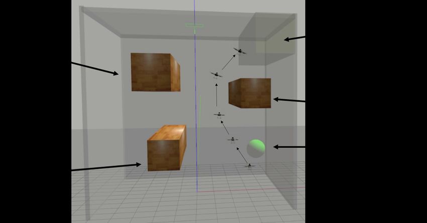
models with high-dimensional state space.                         (S, A, f (·, ·, ·), r(·, ·)), where S is a finite set of states, and
   In this paper, we propose Time-To-Reach (TTR) reward           A is a finite set of actions. f (s, a, s0 ) = Pr(st+1 = s0 |st =
shaping, an approach that integrates optimal control into         s, at = a) is the transition probability that action a in state
model-free RL. This is accomplished by incorporating into         s at time t will lead to state s0 at time t + 1. The reward
the RL algorithm a TTR-based reward function, which is            function r(s, a) represents the immediate reward received if
obtained by solving a Hamilton-Jacobi (HJ) partial differen-      action a is chosen at state s. In this paper, we employ a
tial equation (PDE), a technique that originated in optimal       slight abuse of notation and write
control. A TTR function maps a robot’s internal state to the
minimum arrival time to the goal, assuming a model of the                                 st+1 ∼ f (st , at )                     (1)
robot’s dynamics. In the context of reward function in RL,        to denote that st+1 is drawn from the distribution
intuitively a smaller TTR value indicates a desirable state for   Pr(st+1 |st = s, at = a). This is done to match the notation
many goal-oriented robotic problems.                              of the approximate system dynamics presented in Eq. (3).
   To accommodate the computational intractability of com-           Given an MDP, one aims to find a “policy” denoted π(·)
puting the TTR function for a high-dimensional system such        that specifies the action a = π(s) that is chosen at state s,
as the one used in the RL problem, an approximate, low-           such that the expected sum of discounted rewards
dimensional system model that still captures key dynamic
                                                                                                T
behaviors is selected for the TTR function computation. As                                      X
                                                                                   Rπ (s0 ) =         γ t r(st , π(st ))          (2)
we will demonstrate, such approximate system model is
                                                                                                t=0
sufficient for improving data efficiency of policy learning.
Therefore, our method avoids the shortcomings of both             is maximized over a finite horizon. Here, γ ∈ [0, 1] denotes
model-free RL and optimal control. Unlike model-based RL,         the discount factor and is usually close to 1.
our method does not try to learn and use a full model
                                                                  B. Model-free Reinforcement Learning
explicitly. Instead, we maintain a looser connection between
a known model and the policy improvement process in the              Model-free RL uses algorithms that do not require explicit
form of a TTR reward function. This allows the policy             knowledge of the transition probability distribution associ-
improvement process to take advantage of model information        ated with the MDP to optimize RL objective. An obvious
while remaining robust to model bias.                             advantage of such algorithm is “model-independency” since
   Our approach can be modularly incorporated into any            the MDP model is often inaccessible in the problems with
model-free RL algorithm. In particular, by effectively infus-     high-dimensional state space.
ing system dynamics in an implicit and compatible manner             Policy-based and value-based methods are two main ap-
with RL, we retain the ability to learn policies that map         proaches for training agents with model-free RL. Policy-
sensor inputs directly to actions. Our approach represents        based methods primarily learn a policy by representing it
a bridge between traditional analytical optimal control ap-       explicitly as πθ (a|s) and optimizing the parameters θ either
proaches and the modern data-driven RL, and inherits ben-         directly by gradient ascent on the performance objective
efits of both. We evaluate our approach on two common             J(πθ ) or indirectly by maximizing local approximations of
mobile robotic tasks and obtain significant improvements in       J(πθ ). Policy-based methods sometimes involve “on-policy”
learning performance and efficiency. We choose Proximal           updates which means they update policy only using data
Policy Optimization (PPO) [4], Trust Region Policy Opti-          collected by the most recent version of the policy.
mization (TRPO) [3] and Deep Deterministic Policy Gradient           Value-based methods, on the other hand, primarily learn
(DDPG) [5] as three representative model-free algorithms to       an action-value approximator Qθ (s, a). The optimization is
illustrate the modularity and compatibility of our approach.      sometimes performed in a “off-policy” manner which means
                                                                  it can learn from any trajectory sampled from the same
                   II. PRELIMINARIES                              environment. The corresponding policy is obtained via the
   In this section, we introduce key background concepts of       connection between Q and π: π(s) = arg maxa Qθ (s, a).
this work. Firstly, the Markov Decision Process is described         Among the three model-free RL algorithms in this work,
as the fundamental mathematical framework for modeling            PPO and TRPO fall into the category of policy-based meth-
RL problem. Secondly, model-free RL optimization tech-            ods while DDPG belongs to value-based methods.
niques that are closely related to our work will be presented.    C. Approximate System Model and Time-to-Reach Function
Thirdly, the key concepts of approximate system model and
the mathematical formulation of TTR function are given.             Consider the following dynamical system in Rn
                                                                                         ˙ ) = f˜(s̃(τ ), ã(τ ))
                                                                                        s̃(τ                                      (3)
A. Markov Decision Process
   A Markov Decision Process (MDP) is a discrete time                Note that f˜(·) is used to distinguish this model from f (·)
stochastic control process. It serves as a framework for          in Eq. (1). Here, s̃(·) and ã(·) are the state and action of
modeling decision making in situations where outcomes             an approximate system model. The TTR problem involves
are partly random and partly under the control of deci-           finding the minimum time it takes to reach a goal from any
sion maker. Consider a MDP defined by a 4-tuple M =               initial state s̃, subject to the system dynamics in Eq. (3).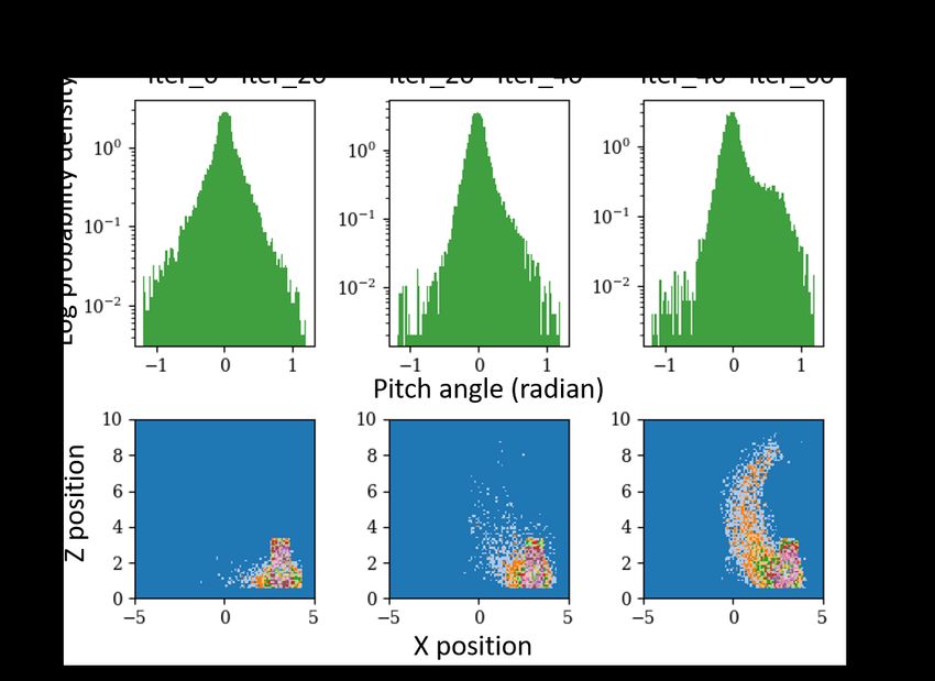
We assume that f˜(·) is Lipschitz continuous. Under these
assumptions, the dynamical system has a unique solution.
The common approach for tackling TTR problems is to
solve a Hamilton-Jacobi (HJ) partial differential equation
(PDE) corresponding to system dynamics and this approach                Fig. 2: Sequential steps of TTR-based reward shaping
is widely applicable to both continuous and hybrid systems
[26]–[28]. Mathematically, the time it takes to reach a goal
Γ ∈ Rn using a control policy ã(·) is
                                                                  A. Model Selection
                 Ts̃ [ã] = min{τ |s̃(τ ) ∈ Γ}              (4)      “Model selection”1 here refers to the fact that we need
                                                                  to pick an (approximate) system model for the robotic task
and the TTR function is defined as follows:                       in order to compute the corresponding TTR function. This
                                                                  model should be relatively low-dimensional so that the TTR
                      φ(s̃) = min Ts̃ [ã]                  (5)
                               ã∈Ã                              computation is tractable but still retain key behaviors in the
                                                                  dynamics of the system.
à is a set of admissible controls in approximate system.            Before the detailed description of model selection, it is
Through dynamic programming, we can obtain φ by solving           necessary to clarify some terminology used in this paper.
the following stationary HJ PDE:                                  First, we use the phrase “full MDP model” to refer to f (·),
                                                                  which drives the real state transitions in the RL problem.
              max{−∇φ(s̃)> f˜(s̃, ã) − 1} = 0              (6)   The full MDP model is often inaccessible since it captures
              ã∈Ã
                                                                  the high-dimensional state inputs including both sensor data
                               φ(s̃) = 0 ∀s̃ ∈ Γ            (7)   and robot internal state. Second, we will use the phrase
                                                                  “approximate system model” to refer to f˜(·). The tilde
Detailed derivations and discussions are presented in [29],
                                                                  indicates that f˜ does not necessarily accurately reflect the
[30]. Normally the computational cost of solving the TTR
                                                                  real state transitions of the problem we are solving. In fact,
problem is too expensive for systems with higher than five
                                                                  the approximate system model should be low-dimensional
dimensional state. However, model simplification and system
                                                                  to simplify the TTR computation while still capturing key
decomposition techniques partially alleviate the computa-
                                                                  robot physical dynamics.
tional burden in a variety of problem setups [31], [32]. Well-
                                                                     The connection between the full MDP model and the
studied level set based numerical techniques [27], [28], [31],
                                                                  approximate system model is formalized as follows. We
[32] have been developed to solve Eq. (6).
                                                                  assume that the approximate system state is a subset of the
                                                                  full MDP state. Thus, the relation between the full MDP
                      III. APPROACH                               state and the approximate model state is
   Model-free RL algorithms have the benefit of being able
to learn control policies directly from high-dimensional state                                  s = (s̃, ŝ)                          (8)
and observation; however, the lack of data efficiency is a
well-known challenge. Integrating a fully MDP model into          Here the full state s refers to the entire high-dimensional
RL seems promising but can sometimes be difficult due to          state in the full MDP model f (·), and s̃ refers to the state of
model bias. In this work, we address this issue by implicitly     the approximate system model f˜(·) which evolves according
utilizing a simplified system model to provide a useful           to Eq. (3). For clarity, we also define ŝ, which are state
“model-informed” reward in an important subspace of the           components in the full MDP model that are not part of s̃.
full MDP state. This way we produce policies that are as flex-       For example, in the simulated car experiment in Section
ible as those obtained from model-free RL algorithms, and         IV-A, the full state contains the internal states of the car, in-
accelerate learning without altering the model-free pattern.      cluding the position (x, y), heading θ, speed v, and turn rate
   In this section, we explain the concrete steps (shown in       ω. In addition, eight laser range measurements d1 , . . . , d8
Fig. 2) of applying our method. The system under consid-          are also part of the state s. These measurements provide
eration may be represented by an MDP given by f (·), as           distances from nearby obstacles. As one can imagine, the
explained in Section II-A; this MDP is in general unknown.        evolution of s can be very difficult if f (·) is impossible to
Choosing an approximate system model f˜(·) that captures          obtain, especially in a priori unknown environments.
key dynamic behavior is the first step; this step is explained       The state of the approximate system, denoted s̃, contains
in Section III-A. Using this approximate system model, we         a subset of the internal states (x, y, θ, v, ω), and evolves
compute the TTR function φ(·), and then apply a simple            according to Eq. (3). In particular, for the simulated results
transformation to it to obtain the reward function r(·) that is   in this paper, we choose the simple Dubins Car model to be
used in RL; this is fully discussed in Section III-B. Finally,
any model-free RL algorithm may be used to obtain a policy         1 Note that “model selection” here has a different meaning than that in
that maximizes the expected return in Eq. (2).                    machine learning.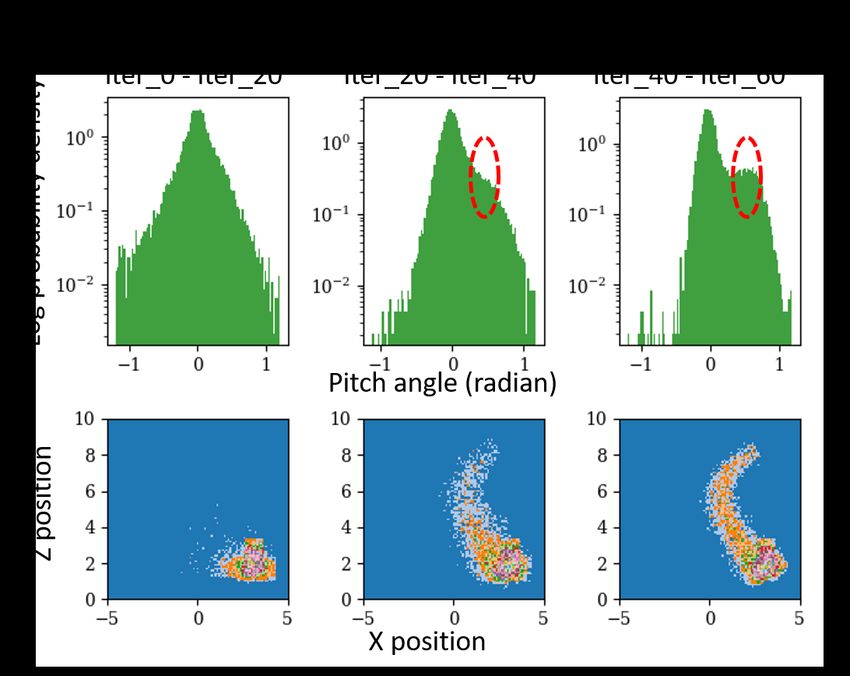
the approximate system dynamics: involved, it is often unclear how to determine an proper
reward for s. As a result, simple reward functions such as
ẋ v cos θ
sparse and distance rewards are sometimes used.
s̃˙ = ẏ = v sin θ (9)
However, this can be easily resolved in our approach by
θ̇ ω
viewing r(·) as a function of s̃, the state of approximate
As we show in Section IV-A, such simple dynamics is system model we have chosen before. As mentioned earlier,
sufficient for improving data efficiency in model-free RL. s̃ a subset of full state s. In our method, the TTR function
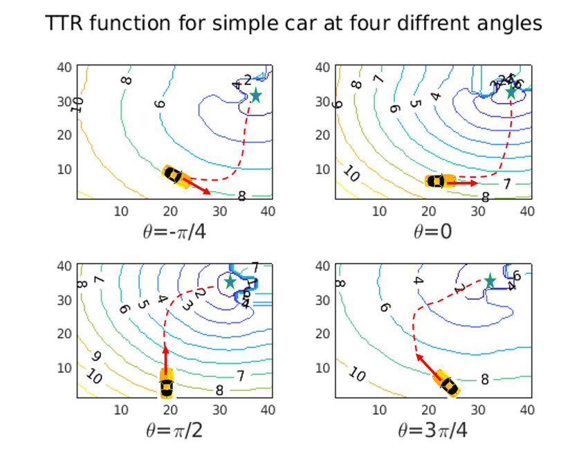
With this choice, the remaining states are denoted ŝ = φ(s̃) defined in Eq. (5) is transformed slightly to obtain the
(v, ω, d1 , . . . , d8 ). Fig. 3 illustrates this example. reward function for full MDP state s:
−φ(s̃) s ∈ I
r(s) = r(s̃, ŝ) = 1000 s∈G (11)
−400 s∈C
By definition, φ(s̃) is non-negative and φ(s̃) = 0 if and only
if s̃ ∈ Γ. Thus, we use −φ(·) as the reward because the state
with lower goal-arrival time should be given a higher reward.
As shown in Eq. (11), we set positive reward for goal states
G and negative reward for collision states C. Note that the
TTR-based reward can also be extended to have obstacles
Fig. 3: State definition of the simulated car in Section IV-A
taken into account, or to satisfy any other design choices if
required. For intermediate states that are neither obstacles or
In general, we may choose s̃ such that a reasonable
goals, TTR function φ(·) directly provides a useful reward
explicit, closed-form ODE model f˜(·) can be derived. Such
signal in an important subspace of the full MDP state. This is
a model should capture the evolution of the robotic internal
significant since the associated rewards for these intermediate
state. One motivation for using an ODE is that the real
states are usually quite difficult to manually design, and
system operates in continuous time, and computing the TTR
TTR reward does not require any manual fine-tuning. This
function for continuous-time systems is a solved problem for
way the RL agent learns faster compared to not having a
sufficiently low-dimensional systems.
useful reward in the subspace, and can quickly learn to
It is worth noting that if a higher-fidelity model of the
generalize the subspace knowledge to the high-dimensional
car is desired, one may also choose the following 5D ODE
observations. For example, positions that are near obstacles
approximate system model instead:
correspond to small values in LIDAR readings, and thus the
ẋ v cos θ
agent would quickly learn these observations correspond to
ẏ v sin θ bad states.
s̃˙ =
To further reduce the computational complexity of solving
θ̇ = ω (10)
v̇ αv the PDE for more complicated system dynamics (such as a
ω̇ αω quadrotor), we may apply system decomposition methods
established from the optimal control community [31]–[33]
In this case, we would have s̃ = (x, y, θ, v, ω), and to obtain an approximate TTR function without significantly
ŝ = (d1 , . . . , d8 ). Note that the choice of an ODE model impacting the overall policy training time. Particularly, we
representing the real robot may be very flexible, depending first decompose the entire system into several sub-systems
on what behavior one wishes to capture. In the 3D car potentially with overlapping components of state variables,
example given in Eq. (9), we focus on modelling the position and then efficiently compute the TTR for each sub-system.
and heading of car to be consistent with the goal. However, We utilize Lax-Friedrichs sweeping-based [27] to compute
if speed and angular speed is deemed crucial for the task the TTR function. As shown in the Table I, computation time
under consideration, one may also choose a more complex of TTR functions are negligible compared to the time it takes
approximate system given by Eq. (10). To re-iterate, a good to train policies.
choice of approximate model is computationally tractable
for the TTR function computation, and captures the system IV. SIMULATED EXPERIMENTS
behaviors that are important for performing the desired task. In order to illustrate the benefits from our TTR-based
reward shaping method, we now present two goal-oriented
B. TTR Function as Approximate Reward tasks through two different mobile robotic systems: a simple
In this section, we discuss how the reward function r(s, a) car and a planar quadrotor. Each system is simulated in
in the full MDP can be chosen based on the TTR function. Gazebo [34], an open-source 3D physical robot simulator.
For simplicity, we ignore a and denote it as r(s), although Also, we utilize the Robot Operating System (ROS) for com-
a simple modification to the TTR function can be made munication management between robot and simulator. For
to incorporate actions into the reward function. Since s is each task, we compare the performance between our TTR-
often in high dimensional space with sensor measurements based reward and two other conventional rewards: sparse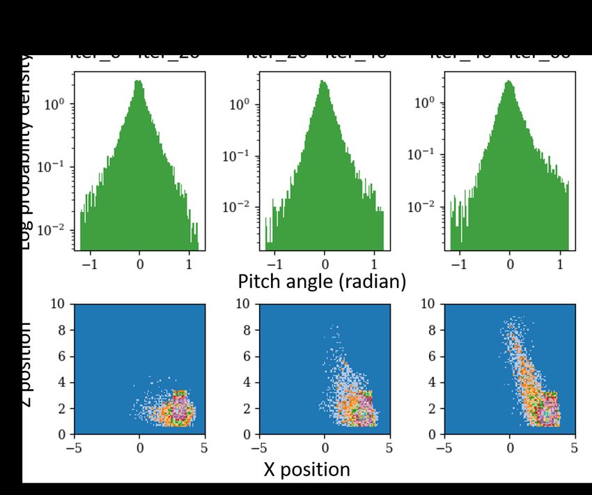
Fig. 4: Performance comparison of three different reward functions on the car example under three model-free RL optimization algorithms:
DDPG, TRPO and PPO. All results are based on the mean of five runs.

            (a) Sparse reward                        (b) Distance reward (the best λ)                      (c) TTR-based reward
Fig. 5: Frequency histograms of (x, z, ψ) during different learning stages on quadrotor task. Top row: log probability density vs. ψ;
bottom row: (x, z) heatmap. Only the TTR-based reward leads to near-complete trajectories in the (x, z) heatmap between iterations 20
and 40, when the other rewards still involve much exploration. Also, the shift (circled in red on Fig. 5c) of log probability density towards
the target θ at 0.75 rad occurs only when TTR-based reward is used, which suggests TTR function is guiding learning effectively.

and distance-based reward. For each reward function, we                        Task           Model     Computation Time    Decomposed
use three representative model-free RL algorithms (DDPG,                     Simple Car      Eq. (9)         5 sec              No
TRPO and PPO) to demonstrate that TTR-based reward can                    Planar Quadrotor   Eq. (12)        90 sec             Yes
be applied to augment any model-free RL algorithm.                      TABLE I: TTR function computational load. ‘Decomposed’ means
   We select sparse and distance-based rewards for com-                 if we need to decompose approximate model into subsystems in
parison with our proposed TTR-based reward because they                 order to reduce computational cost.
are simple, easy to interpret, and easy to apply to any
RL problem. These reward functions are consistent across
our two simulated environments, shown in Table II. We                   sampled initial conditions from the starting area and aims
formulate the distance-based reward as general Euclidean                to reach the goal region without colliding with any obstacle
distance involving position and angle because the tasks we              along the trajectory. Specifically, we set the precise goal state
consider involve reaching some desired set of positions and             as G : (xg = 4 m, yg = 4 m, θg = 0.75 rad), and states
angles, shown in Table II. By choosing different weights λ,             within 0.3 m in positional distance and 0.3 rad in angular
the angle is assigned different weights. For both examples,             distance of G are considered to have reached the goal,
we choose four different weights, λ ∈ {0, 0.1, 1, 10}. The              denoted as Sg = {(x, y, θ)|3.7 m ≤ x ≤ 4.3 m; 3.7 m ≤ y ≤
sparse reward is defined to be 0 everywhere except for goal             4.3 m; 0.45 rad ≤ θ ≤ 1.05 rad}. The TTR-based reward
states (1000 reward) or collision states (−400 reward).                 for this simple car task is derived from a lower-dimensional
                                                                        approximate car system in Eq. (9) which only considers the
A. Simple Car                                                           3D vector (x, y, θ) as state and angular velocity ω as control.
   The car model is widely used as standard testbed in motion              Fig. 4 compares the performance of TTR-based reward
planning [34] and RL [35] tasks. Here we use a “turtlebot-              with sparse and distance-based rewards under three different
2” ground robot to illustrate the performance of the TTR-               model-free algorithms. Success rate after every fixed number
based reward. The state and observation of this example are             of training episodes is considered as qualitative assessment.
already discussed at III-A. The car starts with randomly-               In general, the car system is simpler and more stable thus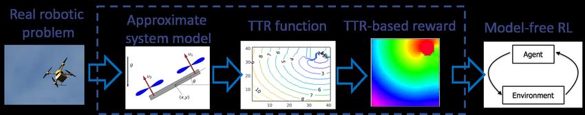
Fig. 6: Performance comparison between TTR, distance and sparse based rewards on quadrotor using three different model-free algorithms.
The results are based on identical evaluation setting as car example and are concluded from five runs as well. Our TTR-based reward
achieves the best in terms of efficiency and performance. Left: success rate comparison under DDPG algorithm Middle: success rate
comparison under TRPO algorithm Right: success rate comparison under PPO algorithm
obtains relatively higher success rate among different re- [36], [37], a popular test subject in the control literature, as
ward settings compared to the quadrotor task (shown later a relatively complex mobile robot to validate that the TTR-
in Fig. 6). In particular, TTR-based reward leads to high based reward shaping method still works well even on highly
success rate (mostly over 90%) consistently with all three dynamic and unstable system. ”Planar” here means the
learning algorithms. In contrast, sparse reward leads to poor quadrotor only flies in the vertical (x-z) plane by changing
performance with PPO, and distance-based reward leads to the pitch angle without affecting the roll and yaw angle.
poor performance with DDPG. The approximate system model has 6D internal state
Note that despite of the better performance from certain s̃ = (x, vx , z, vz , ψ, ω), where x, z, ψ denote the planar
distance-based reward, the choice of appropriate weight for positional coordinates and pitch angle, and vx , vz , ω denote
each variable is non-trivial and not transferable between their time derivatives respectively. The dynamics used for
different tasks. However, TTR-based reward requires little computing the TTR function are given in Eq. (12). The
human engineering to design and can be efficiently computed quadrotor’s movement is controlled by two motor thrusts,
once an low-fidelity model is provided. T1 and T2 . The quadrotor has mass m, moment of inertia
The TTR function for the model in Eq. (9) is shown Iyy , and half-length l. Furthermore, g denotes the gravity
v ψ
in Fig. 1 to convey the usefulness of TTR-based reward acceleration, CD the translation drag coefficient, and CD the
more intuitively. Here, we show the 2D slices of the TTR rotational drag coefficient. Similar to the car example, the
function at four heading angles, θ ∈ {−π/4, 0, π/2, 3π/4}. full state s contains eight laser readings extracted from the
The green star located at the upper-right of each plot is the “Hokoyu utm30lx” ranging sensor for detecting obstacles, in
goal area. The car starts moving from lower-middle area. addition to the internal state s̃. The objective of the quadrotor
Note that the 2D slices look different for different heading is to learn a policy mapping from states and observations to
angles according to the system dynamics, with the contours thrusts that leads it to the goal region.
expanding roughly in opposite direction to the heading slice. vx
ẋ
v̇x −m1
CD v
vx + Tm1 sin ψ + Tm2 sin ψ
Sparse Distance TTR ż v z
s̃˙ = v̇ =
1 v T1 T2 (12)
− (mg + C v ) + cos ψ + cos ψ
∗ ∗
0 −d(·) −φ(s̃) s∈I z D z
m m m
ω
ψ̇
r(s) = 1000 r(s) = 1000 r(s) = 1000 s∈G ψ
1 l l
−400
−400
−400 s∈C ω̇ − Iyy CD ω + Iyy T1 − Iyy T2
(p
2 2 2
∗ d(·) = p(x − xg ) + (y − yg ) + λ(θ − θg ) Simple Car
The environment for this task is shown in Fig. 7. The ob-
(x − xg )2 + (z − zg )2 + λ(ψ − ψg )2 Planar Quadrotor
stacles are fixed. The goal region is Sg = {(x, z, ψ)|3.5 m ≤
∗ φ(s̃): TTR function defined in a subspace of s x ≤ 4.5 m; 8.5 m ≤ z ≤ 9.5 m; 0.45 rad ≤ ψ ≤ 1.05 rad}.
The quadrotor’s starting condition is uniformly-randomly
TABLE II: Reward functions tested in this work. I: set of
intermediate states; G: set of goal states; C: set of collision states.
sampled from {(x, z)|2.5 m ≤ x ≤ 3.5 m; 2.5 m ≤ z ≤
d(·): generalized distance function involving angle. 3.5 m} (green area in Fig. 7) and the starting pitch angle is
randomly sampled from {ψ|−0.17 rad ≤ ψ ≤ 0.17 rad}.
Fig. 6 shows the performance of TTR-based, distance-
B. Planar Quadrotor Model based, and sparse reward under optimization from DDPG,
A Quadrotor is usually considered difficult to control TRPO and PPO. With TTR-based reward, performance is
mainly because of its nonlinear and under-actuated dynamics. consistent over all model-free algorithms. In contrast, sparse
In the second experiment, we select a planar quadrotor model and distance-based rewards often do not lead to quadrotor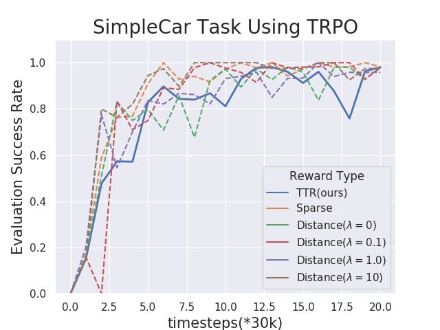
on model-free algorithms can be attached in a compatible
                                                                       way. From the perspective of reward shaping, our approach
                                                                       provides a straight-forward yet distinct shaping option which
                                                                       requires little human engineering.
                                                                         Our method is effective when an explicit robotic system
                                                                       dynamics are accessible. Data efficiency can be greatly
                                                                       improved even if only low-dimensional approximate system
                                                                       dynamics are available.
Fig. 7: Visualization of quadrotor’s sequential movement after
learning from TTR-based reward. The trajectory is connected by a                                    R EFERENCES
combination of the same quadrotor at a few different time snapshots.    [1] M. L. Littman, Algorithms for sequential decision making, 1996.
As shown in the picture, the quadrotor has learned to make use of       [2] A. S. Polydoros and L. Nalpantidis, “Survey of model-based rein-
physical dynamics (tilt) to reach the target as soon as possible            forcement learning: Applications on robotics,” J. Intelligent & Robotic
                                                                            Systems, vol. 86, no. 2, pp. 153–173, May 2017.
                                                                        [3] J. Schulman, F. Wolski, P. Dhariwal, A. Radford, and
                                                                            O. Klimov, “Proximal policy optimization algorithms,” CoRR,
stability and consistency of performance. For example, under                vol. abs/1707.06347, 2017.
sparse and distance-based rewards, performance is relatively            [4] J. Schulman, S. Levine, P. Moritz, M. Jordan, and P. Abbeel, “Trust
                                                                            region policy optimization,” in Proc. Annual Int. Conf. Machine
good under TRPO, but very poor under DDPG. In terms of                      Learning, 2015.
learning efficiency, TTR-based reward achieves a success rate           [5] T. P. Lillicrap, J. J. Hunt, A. Pritzel, N. Heess, T. Erez, Y. Tassa,
of greater than 90% after 3 iterations (approximately 90000                 D. Silver, and D. Wierstra, “Continuous control with deep reinforce-
                                                                            ment learning,” arXiv preprint arXiv:1509.02971, 2015.
time steps) regardless of the model-free algorithm. This is             [6] R. S. Sutton and A. G. Barto, Reinforcement Learning: An Introduc-
the best result among the three reward functions we tested.                 tion. USA: A Bradford Book, 2018.
   To further illustrate the effectiveness of our approach,             [7] J. Schmidhuber, “Deep learning in neural networks: An overview,”
                                                                            Neural Networks, vol. 61, pp. 85 – 117, 2015.
Fig. 5 shows statistics of positional (x, z) and angular                [8] Y. Lecun, Y. Bengio, and G. Hinton, “Deep learning,” Nature, vol.
variables ψ during early learning stages using the three                    521, pp. 436–444, May 2015.
reward functions over three ranges of learning iterations.              [9] I. Osband, B. Van Roy, D. Russo, and Z. Wen, “Deep exploration via
                                                                            randomized value functions,” arXiv preprint arXiv:1703.07608, 2017.
Note that we choose distance-based reward with λ = 10                  [10] A. Guez, D. Silver, and P. Dayan, “Efficient bayes-adaptive reinforce-
since it’s the best one among all tested distance-based reward              ment learning using sample-based search,” in Advances in Neural
variants. The 2D histograms show the frequency of (x, z)                    Information Processing Systems 25, F. Pereira, C. J. C. Burges,
                                                                            L. Bottou, and K. Q. Weinberger, Eds. Curran Associates, Inc., 2012,
along trajectories in training episodes as heatmaps while the               pp. 1025–1033.
1D histograms show the frequency of ψ as log probability               [11] O. Nachum, S. S. Gu, H. Lee, and S. Levine, “Data-efficient hier-
densities. Note that the second column of each subplot (from                archical reinforcement learning,” in Advances in Neural Information
                                                                            Processing Systems, 2018, pp. 3303–3313.
iteration 20 ∼ 40) represents transitory behaviors, before the         [12] H. Tang, R. Houthooft, D. Foote, A. Stooke, O. X. Chen, Y. Duan,
quadrotor successfully learns to perform the task. Fig. 5c                  J. Schulman, F. DeTurck, and P. Abbeel, “#exploration: A study of
shows that the desired angular goal (ψ = 0.75 rad) has higher               count-based exploration for deep reinforcement learning,” in Advances
                                                                            in neural information processing systems, 2017, pp. 2753–2762.
probability density (circled in red), which means TTR-                 [13] A. Vezhnevets, V. Mnih, S. Osindero, A. Graves, O. Vinyals, J. Aga-
based reward does provide effective angular local feedback.                 piou et al., “Strategic attentive writer for learning macro-actions,” in
Furthermore, heat maps for TTR-based reward (Fig. 5c) is                    Advances in neural information processing systems, 2016, pp. 3486–
                                                                            3494.
concentrated around plausible trajectories for reaching the            [14] A. S. Vezhnevets, S. Osindero, T. Schaul, N. Heess, M. Jaderberg,
goal, while heat maps for the other rewards are more spread                 D. Silver, and K. Kavukcuoglu, “Feudal networks for hierarchical
out. This shows TTR-based reward is providing dynamics-                     reinforcement learning,” in Proceedings of the 34th International
                                                                            Conference on Machine Learning-Volume 70. JMLR. org, 2017, pp.
informed guidance.                                                          3540–3549.
                                                                       [15] Y. Bengio, J. Louradour, R. Collobert, and J. Weston, “Curriculum
                      V. CONCLUSION                                         learning,” in Proc. Annual Int. Conf. Machine Learning, 2009.
                                                                       [16] C. Florensa, D. Held, M. Wulfmeier, and P. Abbeel, “Reverse
   In this paper, we propose TTR-based reward shaping to                    curriculum generation for reinforcement learning,” CoRR, 2017.
alleviate the data inefficiency of model-free RL on robotic                 [Online]. Available: http://arxiv.org/abs/1707.05300
tasks. By using TTR function to provide RL reward, the                 [17] C. G. Atkeson, A. W. Moore, and S. Schaal, “Locally weighted
                                                                            learning for control,” in Lazy learning. Springer, 1997, pp. 75–113.
model-free learning process remains flexible but is endued             [18] P. Abbeel, A. Coates, M. Quigley, and A. Y. Ng, “An application of
with global guidance provided by implicit system dynamics                   reinforcement learning to aerobatic helicopter flight,” in Advances in
priors. In this approach, an approximate system model cho-                  neural information processing systems, 2007, pp. 1–8.
                                                                       [19] M. Deisenroth and C. E. Rasmussen, “Pilco: A model-based and
sen in a highly flexible way. By computing a TTR function                   data-efficient approach to policy search,” in Proceedings of the 28th
based on the chosen model and integrating it as the RL                      International Conference on machine learning (ICML-11), 2011, pp.
reward function, the agent receives more dynamics-informed                  465–472.
                                                                       [20] F. Lin and R. D. Brandt, “An optimal control approach to robust
feedback and learns faster and better.                                      control of robot manipulators,” IEEE Transactions on Robotics and
   Simple and effective, TTR-based reward shaping is easy to                Automation, vol. 14, no. 1, pp. 69–77, 1998.
implement and can be used as a wrapper for any model-free              [21] S. Wang and K. Hauser, “Realization of a real-time optimal control
                                                                            strategy to stabilize a falling humanoid robot with hand contact,”
RL algorithm since it does not alter the original algorithmic               in 2018 IEEE International Conference on Robotics and Automation
structure. Accordingly, any additional tricks or improvements               (ICRA), May 2018, pp. 3092–3098.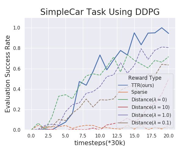
[22] M. Chen and C. J. Tomlin, “Hamilton–jacobi reachability: Some
     recent theoretical advances and applications in unmanned airspace
     management,” Annual Review of Control, Robotics, and Autonomous
     Systems, vol. 1, pp. 333–358, 2018.
[23] M. Chen, Q. Hu, J. F. Fisac, K. Akametalu, C. Mackin, and C. J.
     Tomlin, “Reachability-based safety and goal satisfaction of unmanned
     aerial platoons on air highways,” Journal of Guidance, Control, and
     Dynamics, vol. 40, no. 6, pp. 1360–1373, 2017.
[24] M. Chen, J. F. Fisac, S. Sastry, and C. J. Tomlin, “Safe sequential path
     planning of multi-vehicle systems via double-obstacle hamilton-jacobi-
     isaacs variational inequality,” in 2015 European Control Conference
     (ECC). IEEE, 2015, pp. 3304–3309.
[25] M. Chen, J. C. Shih, and C. J. Tomlin, “Multi-vehicle collision
     avoidance via hamilton-jacobi reachability and mixed integer program-
     ming,” in 2016 IEEE 55th Conference on Decision and Control (CDC).
     IEEE, 2016, pp. 1695–1700.
[26] Z. Zhou, R. Takei, H. Huang, and C. J. Tomlin, “A general, open-loop
     formulation for reach-avoid games,” in Proc. IEEE Conf, Decision and
     Control, 2012.
[27] I. Yang, S. Becker-Weimann, M. J. Bissell, and C. J. Tomlin, “One-
     shot computation of reachable sets for differential games,” in Proc.
     ACM Int. Conf. Hybrid Systems: Computation and Control, 2013.
[28] R. Takei and R. Tsai, “Optimal trajectories of curvature constrained
     motion in the hamilton–jacobi formulation,” J. Scientific Computing,
     vol. 54, no. 2, pp. 622–644, Feb 2013.
[29] M. Bardi and I. Capuzzo-Dolcetta, Optimal Control and Viscosity Solu-
     tions of Hamilton-Jacobi-Bellman Equations, ser. Modern Birkhäuser
     Classics, 2008.
[30] M. Bardi and P. Soravia, “Hamilton-jacobi equations with singular
     boundary conditions on a free boundary and applications to differential
     games,” Transactions of the American Mathematical Society, vol. 325,
     no. 1, pp. 205–229, 1991.
[31] I. M. Mitchell, “The flexible, extensible and efficient toolbox
     of level set methods,” J. Scientific Computing, vol. 35, no. 2, pp. 300–
     329, Jun 2008.
[32] M. Chen, S. Herbert, and C. J. Tomlin, “Fast reachable set approxima-
     tions via state decoupling disturbances,” in Proc. IEEE Conf. Decision
     and Control, 2016.
[33] M. Chen, S. L. Herbert, M. S. Vashishtha, S. Bansal, and C. J. Tomlin,
     “Decomposition of reachable sets and tubes for a class of nonlinear
     systems,” IEEE Transactions on Automatic Control, vol. 63, no. 11,
     pp. 3675–3688, Nov 2018.
[34] N. Koenig and A. Howard, “Design and use paradigms for gazebo,
     an open-source multi-robot simulator,” in Proc. IEEE/RSJ Int. Conf.
     Intelligent Robots and Systems, 2004.
[35] D. J. Webb and J. van den Berg, “Kinodynamic rrt*: Asymptotically
     optimal motion planning for robots with linear dynamics,” in Proc.
     IEEE Int.Conf. Robotics and Automation, 2013.
[36] J. H. Gillula, H. Huang, M. P. Vitus, and C. J. Tomlin, “Design of
     guaranteed safe maneuvers using reachable sets: Autonomous quadro-
     tor aerobatics in theory and practice,” in 2010 IEEE International
     Conference on Robotics and Automation. IEEE, 2010, pp. 1649–
     1654.
[37] S. Singh, A. Majumdar, J.-J. Slotine, and M. Pavone, “Robust online
     motion planning via contraction theory and convex optimization,” in
     2017 IEEE International Conference on Robotics and Automation
     (ICRA). IEEE, 2017, pp. 5883–5890.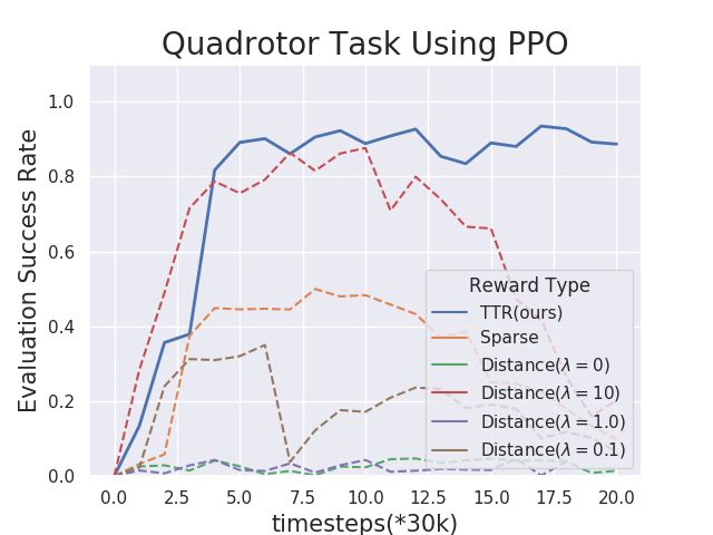

You can also read