Statistical Methods in Bidding Decision Support for Construction Companies
←
→
Page content transcription
If your browser does not render page correctly, please read the page content below
applied
              sciences
Article
Statistical Methods in Bidding Decision Support for
Construction Companies
Agnieszka Leśniak

                                          Faculty of Civil Engineering, Cracow University of Technology, 31-155 Krakow, Poland; alesniak@l7.pk.edu.pl

                                          Abstract: On the border of two phases of a building life cycle (LC), the programming phase (concep-
                                          tion and design) and the execution phase, a contractor is selected. A particularly appropriate method
                                          of selecting a contractor for the construction market is the tendering system. It is usually based on
                                          quality and price criteria. The latter may involve the price (namely, direct costs connected with works
                                          realization as well as mark-ups, mainly overhead costs and profit) or cost (based on the life cycle
                                          costing (LCC) method of cost efficiency). A contractor’s decision to participate in a tender and to
                                          calculate a tender requires an investment of time and company resources. As this decision is often
                                          made in a limited time frame and based on the experience and subjective judgement of the contractor,
                                          a number of models have been proposed in the literature to support this process. The present paper
                                          proposes the use of statistical classification methods. The response obtained from the classification
                                          model is a recommendation to participate or not. A database consisting of historical data was used
                                          for the analyses. Two models were proposed: the LOG model—using logit regression and the LDA
                                          model—using linear discriminant analysis, which obtain better results. In the construction of the
                                          LDA model, the equation of the discriminant function was sought by indicating the statistically
                                          significant variables. For this purpose, the backward stepwise method was applied, where initially

                                          all input variables were introduced, namely, 15 identified bidding factors, and then in subsequent
                                   steps, the least statistically significant variables were removed. Finally, six variables (factors) were
Citation: Leśniak, A. Statistical        identified that significantly discriminate between groups: type of works, contractual conditions,
Methods in Bidding Decision Support       project value, need for work, possible participation of subcontractors, and the degree of difficulty of
for Construction Companies. Appl.         the works. The model proposed in this paper using a discriminant analysis with six input variables
Sci. 2021, 11, 5973. https://doi.org/     achieved good performance. The results obtained prove that it can be used in practice. It should
10.3390/app11135973                       be emphasized, however, that mathematical models cannot replace the decision-maker’s thought
                                          process, but they can increase the effectiveness of the bidding decision.
Academic Editor: Igal M. Shohet

                                          Keywords: bidding decision; LCC criterion; price criterion; construction; statistical method; classifi-
Received: 26 May 2021
                                          cation; probability of winning
Accepted: 24 June 2021
Published: 27 June 2021

Publisher’s Note: MDPI stays neutral
                                          1. Introduction
with regard to jurisdictional claims in
published maps and institutional affil-         With the development of new technologies and advanced building materials, an
iations.                                  increasing number of demands are placed on the construction industry. Modern buildings
                                          should have as little impact as possible on the environment [1–3] using sustainable materials
                                          (such as natural or recycled materials) [4–6] and environmentally friendly construction
                                          technologies [7–9]. They should have low energy consumption [10,11], demonstrate the
Copyright: © 2021 by the author.
                                          ability to perform repairs resulting from wear and tear [12–14], as well as from possible
Licensee MDPI, Basel, Switzerland.
                                          breakdowns [15,16]. Preferably, they should allow the recycling or disposal [17,18] of
This article is an open access article
                                          the resulting construction waste. These aspects are considered by the participants in the
distributed under the terms and           investment process, both the investor, the contractor, and the user against the background
conditions of the Creative Commons        of the different stages of the building life cycle. Phases identified in the literature include
Attribution (CC BY) license (https://     the following: the programming phase (study and conceptual analysis, as well as design),
creativecommons.org/licenses/by/          the execution phase (construction of the facility), the operation phase (operation, use, and
4.0/).                                    maintenance of the facility) and the decommissioning phase (demolition of the facility). In

Appl. Sci. 2021, 11, 5973. https://doi.org/10.3390/app11135973                                               https://www.mdpi.com/journal/applsci
Appl. Sci. 2021, 11, 5973 2 of 14
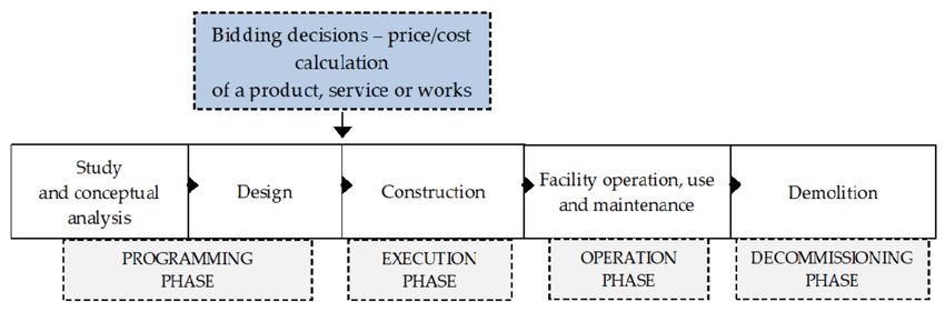
this paper, attention is paid to the programming phase, and in particular to the conclusion
of the design phase, which must be followed here by the selection of the contractor for the
construction work before the execution phase begins (Figure 1).
Figure 1. Bidding decisions of the building contractor within the building life cycle.
The methods of sourcing contractors in the construction market depend on the type of
market (private or public sector) and the value of the project. Due to the individualized
nature of construction production and the long production cycle, the tendering system is
particularly suited to the operating conditions of the construction market [19]. The bidding
procedure ensures that competition takes place properly and that its results are objective.
It is also a factor conditioning the objectivity of prices in the construction industry. Bidding
can be carried out by any investor looking for a contractor, but it is the potential contractor
who must decide to tender and begin the laborious process of preparing a bid.
The selection of the most advantageous tender is normally based on quality and
price criteria [20]. The price criterion may involve a price or cost and is based on a cost-
effectiveness method, such as life-cycle costing (LCC). In the former case, the basis for
determining a price are the direct costs connected with works realization as well as mark-
ups, mainly overhead costs and profit [21–23]. In the latter case, life cycle costs (LCC)
should be estimated, including the costs for planning, design, operation, maintenance,
and decommissioning minus the residual value, if there is any [24]. In the literature, one
can find many mathematical models prepared for the estimation of building life cycle
costs [25–27], the description and comparison of which can be found, for example, in [28].
A contractor’s decision to enter a tender requires action to prepare the tender and requires
investment of time and commitment of staff, that is, the direct use of company resources.
Irrespective of the outcome of the tender, the costs of preparing the tender will be incurred.
Efficient bidding is certainly essential for every construction company. Choosing the right
tender for a company has an impact on the creation of its image, its financial condition,
and its aspiration to success [29].
The decision to participate in a tender often must be made by the contractor within
a limited time frame and it is often based on his or her own experience. To improve
the effectiveness of the decision, various models have been developed to support this
process. In this case, a bidding decision model should be understood as a mathematical
representation of reality, with a proposed technique to help the construction contractor
decide to participate in the tender, avoiding errors and randomness. Efficient decision
making is one of the greatest challenges of contemporary construction [30].
Different methods and tools are used to build models supporting construction con-
tractors’ decisions to bid. A summary of the selected existing (published after 2000) models
is provided in Table 1.Appl. Sci. 2021, 11, 5973 3 of 14
Table 1. Examples of models supporting tender decisions presented in the literature after 2000.
Bidding Decision Model Authors Source Year of Publication
Model based on Case-based reasoning approach Chua D.K.H, Li D.Z, Chan W.T. [31] 2001
Model based on the Analytical Hierarchy Process
Cagno E., Caron F., Perego A. [32] 2001
(AHP) method
Model based on artificial neural network Wanous M., Boussabaine A. H., Lewis J. [33] 2003
Model based on fuzzy linguistic approach Lin Ch.-T., Chen Y.-T. [34] 2004
Model based on logistic regression Drew D., Lo H.P. [35] 2007
Model based on a knowledge system Egemen M., Mohamed A. [36] 2008
Model based on data envelopment analysis (DEA) El-Mashaleh M. S. [37] 2010
Model based on a multi-criteria analysis and fuzzy set Cheng M.-Y., Hsiang C. Ch., Tsai H.-Ch,
[38] 2011
theory Do H.-L.
Model based on an ant colony optimisation algorithm
Shi, H. [39] 2012
and artificial neural network
Model based on fuzzy Analytical Hierarchy Process
Chou, J. S., Pham, A. D., Wang, H. [40] 2013
and regression-based simulation
Model based on a fuzzy set theory Leśniak, A., Plebankiewicz, E. [41] 2016
Model based on RBF neural networks Leśniak, A. [42] 2016
Model based on the simple additive weighted scoring Chisala, M. L. [43] 2017
Leśniak, A., Kubek, D., Plebankiewicz,
Model based on the fuzzy AHP [44] 2018
E., Zima, K., Belniak, S.
Arya, A., Sisodia, S., Mehroliya, S.,
Model based on the game theory [45] 2020
Rajeshwari, C. S.
Ojelabi, R. A., Oyeyipo, O. O., Afolabi,
Model based on structural equation [46] 2020
A. O., Omuh, I. O.
Model Based on Projection Pursuit Learning Method Zhang, X., Yu, Y., He, W., Chen, Y. [47] 2021
It is worth noting that the indicated models differ in the methods used. Different
methods, techniques, and approaches are sought and applied to obtain the most effective
models. What is important, continuously for at least 20 years, modeling of a tender decision
is still an object of research and interest of researchers.
The models proposed in the literature are generally based on factors, also called
criteria, affecting the decision, and using them as input parameters. The number of
publications on the identification of factors is considerable, as each country and region
has a certain characteristic group of factors that will not be found in other markets [48–50].
It can therefore be concluded that the factors influencing tender decisions depend not
only on the project to be tendered but also on the environment and market in which the
contractor operates.
Bidding problems are also known in procurement auctions [51,52]. This paper [53]
presents the analysis of the relation between the award price and the bidding price in
the case of public procurement in Spain. An award price estimator was proposed as it is
believed to be particularly useful for companies and public procurement agencies. Procure-
ment auctions have long been employed in the logistics and transportation industry [54].
In combinatorial auctions, each carrier must determine the set of profitable contracts to
bid on and the associated ask prices. This is known as the bid construction problem
(BCP) [55]. Different approaches for the bid construction problem (BCP) in transportation
procurement auctions are proposed in literature. One of them can be found in [56] where
authors proposed solving the BCP problem for heterogeneous truckload using exact and
heuristic methods.Appl. Sci. 2021, 11, 5973 4 of 14
The paper proposes the use of statistical methods to support the decision-making
process of a construction contractor related to the preparation of a price offer and entering
a tender. Two classification methods were used as decision support models. The response
obtained from the classification model is a recommendation to participate in the tender
(qualification into the W-winning class), or a recommendation to resign (allocation into the
L-losing class). To perform the analyses, it was necessary to use a database consisting of
historical data, that is, resolved tenders. The research framework diagram is presented in
Figure 2.
Figure 2. The research framework diagram.
2. Materials and Methods
2.1. Data Acquisition
In [57], a literature survey and research gap analysis of statistical methods used in the
context of optimizing bids were presented. The paper attempts to build a decision-making
model using two statistical methods: regression analysis and discriminant analysis. In
the methods derived from regression analysis, the values of the Y variable (the explained
variable) are given before determining the model and based on them and the adopted
factors, the parameters of the model are determined. However, in the case of discriminant
analysis, the values of the variable are obtained when the model is determined.
Factors influencing decision-making were proposed as input parameters of the mod-
els (explanatory variables). As a result of research (a questionnaire survey) conducted
by the author in Poland, presented and described in previous works [29,44], 15 factors
were identified: x1 —type of works, x2 —experience in similar projects, x3 —contractual
conditions, x4 —investor reputation, x5 —project value, x6 —need for work, x7 —the size of
the project, x8 —profits made in the past from similar undertakings, x9 —duration of the
project, x10 —tender selection criteria, x11 —project location, x12 —time to prepare the offer,
x13 —possible participation of subcontractors, x14 —the need for specialized equipment,
and x15 —degree of difficulty of the works. The tender score was the model output variable
(Y) representing the class:
• W—win—interpreted as a recommendation to take part in a tender,
• L—loss—interpreted as a recommendation to abandon the tender.
The starting point for the selected methods was the construction of a database. The
research performed in Poland was of primary nature, based on information collected to
solve a given decision problem. With regard to the type of research material, the study
comprised quantitative research (evaluation of factors) and qualitative research: determi-
nation of the result obtained by the contractor in a given evaluated tender. The factorsAppl. Sci. 2021, 11, 5973 5 of 14
identified were used to evaluate the tenders entered into by the contractors participating
in the research. Each factor, from x1 to x15 , was rated on a scale from 1 to 7, where the
numbers meant 1—very unfavorable, and 7—very favorable influence of the factor on
the decision to participate in the tender. This scale has already been used successfully in
previous works [44]. The result for each tender evaluated was then recorded (W—win,
L—loss). In the end, the database contained 88 evaluated tenders, of which 64 were lost
cases (L) and 24 won cases (W). Selected database records of evaluated tenders including
factor evaluations with the corresponding result obtained in the tender (W—win, L—loss,)
are presented in Table 2.
Table 2. Selected database records.
Record
(Evaluated Factors Result
Tender)
i x1 x2 x3 x4 x5 x6 x7 x8 x9 x10 x11 x12 x13 x14 x15
4 6 7 5 5 3 6 3 4 5 3 6 5 2 6 7 L
12 4 6 5 6 1 6 1 4 6 5 6 6 7 3 5 W
62 7 7 4 4 4 5 3 4 5 3 5 5 4 6 6 L
2.2. Regression Analysis Model
The main task of the qualitative decision-making model will be to determine the
probability of the contractor’s success in the tender (winning) and to identify variables that
significantly affect the outcome of the tender. A binomial (dichotomous) model is sought in
which the explanatory variable Y is quantified by a zero-one variable. It takes two possible
variants described by the codes “1”—W (win) and “0”—L (loss). If pi is the probability of
the event Yi = 1, then 1 − pi is the probability of the event Yi = 0. The expected value of the
variable Yi is [58,59]:
E(Yi ) = 1· pi + 0·(1 − pi ) = pi (1)
In binomial models, it is assumed that pi is a function of the vector of values of the
explanatory variables xi for the i-th object and the parameter vector β [58,59]:
Pi = P(yi = 1) = F xiT β (2)
Depending on the type of F-function, different types of models are distinguished [60]: a
linear probability model, logit model, and probit model. Using the simplest of the binomial
models—the linear probability model—has many negative consequences described in
the literature [58,61]. Probit and logit models, on the other hand, as indicated by some
authors [60], are similar to each other and in practice one of them is used. Therefore, the
search for a binomial model for the phenomenon in question was limited to a logistic
regression model. The general form of the logit model is as follows [58,59]:
pi
Yi∗ = ln = β 0 α0 + β 1 X1i + β 2 xX2i + · · · + β k Xki + ui (3)
1 − pi
where:
β j —structural model parameters,
ui —random component,
p
ln 1−ip —logit,
i
Yi∗ —unobservable qualitative variable,
X ji —the values of the explanatory variables of the model,
pi —the probability of taking the value “1” by the dependent variable Yi calculated from
the logistic distribution density function.Appl. Sci. 2021, 11, 5973 6 of 14
0
e xi β 1 1
pi = Xi0 β
= − Xi0 β
= (4)
1+e 1+e 1 + e−( β0 + β1 X1i + β2 X2i +···+ β k Xki )
Unobservable variable Yi∗ is defined as a latent variable, as one can observe only the
binary variable Yi in the form:
1; Yi∗ > 0
Yi = (5)
0; Yi∗ ≤ 0
Logit according to [53], denotes the odds ratio of accepting to not accepting the value
“1” for the variable Yi . It takes the value zero if pi = 0.5. In the case when pi < 0.5, the
odds ratio takes a negative value, and when pi > 0.5, a positive one.
2.3. Discriminant Analysis Model
Linear discriminant analysis (LDA), presented in 1936 [62], enables the classification of
cases (objects) into one of the predetermined groups based on explanatory variables (case
characteristics). The use of linear discriminant analysis to classify objects (cases) [63] or
supporting decision-making processes [64] are commonly found in the literature. The aim
of discriminant methods is to determine which of the explanatory variables differentiate
groups the most. The discrimination problem can be solved by means of discriminant
functions which are most often linear functions of input variables characterizing the
cases [65]. If group sizes are not comparable, a modified form of the discriminant function
should be used [65]:
nr
Kr = cro + cr1 X1 + cr2 X2 + . . . + crm Xm + ln , (6)
n
where:
Kr —classification function (for the r-th group of cases),
crj —the coefficient of the r-th classification function with j-th input variable of significant
discriminatory power, j = 0, 1, . . . , m’,
cro = lnpri —absolute term, probability pi means the a priori probability of qualifying the i-th
object to the r-th group,
nr —denotes the size of a given group,
n—sample size.
Modeling takes place in several stages. In the first step of building the model, the
discriminant function equation is sought by identifying variables that significantly dis-
criminate groups. The next step is to check the statistical significance of the discriminant
function and determine its coefficients. The next stage of the analysis is a classification
procedure using classification functions.
2.4. Evaluation of the Proposed Models
To assess the quality and relevance of the performance of the proposed classification
models [66], the following were proposed:
• A relevance matrix that indicates the number and often the proportion of correctly
and incorrectly classified cases;
• Diagnostic test parameters: sensitivity (7), specificity (8), positive (9), and negative
(10) predictive value, test reliability (11) based on the contingency matrix:
Sensitivity indicates the ratio of true positives to the sum of true positives and false
negatives. In the problem under analysis, it describes the ability to detect the winning cases.
TP
sensitivity = (7)
TP + FNAppl. Sci. 2021, 11, 5973 7 of 14
Specificity means the ratio of true negatives to the sum of true negatives and false
positives. In the problem examined, it describes the ability to detect the losing cases.
TN
Speci f icity = (8)
TN + FP
PPV (positive predictive value) denotes the probability that the case identified by the
classifier as winning is indeed a winning case.
TP
PPV = (9)
TP + FP
NPV (negative predictive value) stands for the probability that the case identified by
the classifier as loss is indeed a losing case.
TN
NPV = (10)
FN + TN
Effectiveness of the decision rule ACC (accuracy) implies the extent to which the
results of the study reflect reality.
TP + TN
ACC = (11)
TP + TN + FP + FN
where:
TP—true positive results,
FP—false positive results,
TN—false negative results,
FN—true negative results.
3. Results and Discussion
3.1. LOG Model—The Model Using Regression Analysis
Using logit regression, an attempt was made to estimate the qualitative variable Y,
also trying to explain which factors, with what strength and in what direction, affect the
chance of a tender success (Y). The parameter estimates are summarized in Table 3.
By analyzing the obtained results with the assumed significance level α = 0.1, only two
variables significantly affect the model: x3 —contractual conditions and x6 —need for work.
However, the p value for the variables x12 —time to prepare the offer and x15 —the degree
of difficulty of the works, are slightly higher than 0.1, so it was decided to include these
variables and recalculate the model. The parameter estimates for the logistic regression
model (with four explanatory variables) are summarized in Table 4.
Finally, three variables were left (the non-significant variable x12 —time to prepare an
offer, was discarded) and recalculations were made.
The parameter estimates for the logistic regression model (with three explanatory
variables) are summarized in Table 5.
The form of the proposed logit model (LOG model) is as follows:
pi
Ŷi = ln = −0.9532· x3 − 2.2877· x6 + 0.6012· x15 + 15.9217 (12)
1 − pi
This means that the probability pi (that is, situation Yi = 1) is estimated as:
exp(−0.9532· x3 − 2.2877· x6 + 0.6012· x15 + 15.9217)
p̂i = (13)
1 + exp(−0.9532· x3 − 2.2877· x6 + 0.6012· x15 + 15.9217)
Statistical verification of the logit model consisting in determining the degree of
the model fitting the data and testing the statistical significance of the parameters was
successful. The odds quotient is 9.62 and is higher than 1 which means that the classificationAppl. Sci. 2021, 11, 5973 8 of 14
is nine times better than what would be expected by chance. Using the proposed logit
model, it is possible to estimate the probability with which a given tender will be won.
Table 3. Parameter estimates for the logit model—15 explanatory variables.
Dependent
Standard Statistically
Variable Y Coefficient β Walda Stat. p Value
Error Significant *
RESULT
Absolute
181.2342 101.4030 3.1943 0.0739 *
term
x1 −0.8114 2.1518 0.1422 0.7061
x2 −0.4787 1.2390 0.1493 0.6992
x3 −6.4249 2.8502 5.0814 0.0242 *
x4 1.0285 1.2892 0.6364 0.4250
x5 0.6708 1.5074 0.1980 0.6563
x6 −6.6233 2.5664 6.6607 0.0099 *
x7 −1.2769 1.5475 0.6809 0.4093
x8 −4.1032 6.4537 0.4042 0.5249
x9 0.8568 1.1536 0.5516 0.4577
x10 −3.3306 2.8215 1.3935 0.2378
x11 −2.9788 2.2852 1.6992 0.1924
x12 3.5272 2.3601 2.2335 0.1350
x13 −15.8525 11.8791 1.7808 0.1820
x14 −2.4435 2.2014 1.2320 0.2670
x15 4.9962 3.4396 2.1098 0.1464
* Significance level α = 0.1
Table 4. Parameter estimates for the logit model—four explanatory variables.
Dependent
Standard Statistically
Variable Y Coefficient β Walda Stat. p Value
Error Significant *
RESULT
Absolute
16.1289 4.6709 11.9235 0.0006 *
term
x3 16.1289 4.6709 11.9235 0.0006 *
x6 −0.9145 0.4582 3.9833 0.0460 *
x12 −2.2736 0.5790 15.4179 0.0001
x15 −0.0840 0.5715 0.0216 0.8831 *
* Significance level α = 0.1
Table 5. Parameter estimates for the logit model—three explanatory variables.
Dependent
Standard Statistically
Variable Y Coefficient β Walda Stat. p Value
Error Significant *
RESULT
Absolute
15.9217 4.4375 12.8739 0.0003 *
term
x3 −0.9532 0.3769 6.3964 0.0114 *
x6 −2.2877 0.5723 15.9812 0.0001 *
x15 0.6012 0.3271 3.3777 0.0661 *
* Significance level α = 0.1
3.2. LDA Model—The Model Using Discriminant Analysis
In the first step of building the model, the equation of the discriminant function was
searched for, indicating variables that significantly discriminate groups. To achieve this,
the backward stepwise method was applied. In this approach, all variables are entered into
the model (step 0) and then, in subsequent steps, one variable that is the least statistically
significant is removed. Results with all 15 input variables (step 0) indicated at the assumedAppl. Sci. 2021, 11, 5973 9 of 14
significance level α = 0.1, that only four variables significantly discriminate between groups
(x3 , x5 , x6 , x13 ).
The results for the model and the evaluation of all 15 input variables (step 0) are given
in Table 6.
Table 6. Evaluation of the parameters of the discriminant function—15 explanatory variables.
Wilks’ Partial Lambda The Value of the F Statistically
Variables p Value Tolerance 1-Tolerance
Lambda Wilks Statistic Significant *
x1 0.430141 0.961162 2.90937 0.092377 0.377706 0.622294
x2 0.413447 0.999971 0.00207 0.963850 0.370875 0.629125
x3 0.449346 0.920082 6.25390 0.014669 0.376703 0.623297 *
x4 0.421275 0.981391 1.36523 0.246487 0.522505 0.477495
x5 0.454559 0.909531 7.16170 0.009215 0.109267 0.890733 *
x6 0.609746 0.678045 34.18763 0.000000 0.643071 0.356929 *
x7 0.419668 0.985148 1.08548 0.300962 0.096009 0.903991
x8 0.434939 0.950558 3.74495 0.056895 0.577896 0.422104
x9 0.414878 0.996522 0.25127 0.617712 0.757040 0.242960
x10 0.417598 0.990032 0.72491 0.397361 0.672704 0.327296
x11 0.424018 0.975042 1.84297 0.178843 0.633470 0.366531
x12 0.430727 0.959854 3.01140 0.086960 0.512083 0.487917
x13 0.444633 0.929835 5.43308 0.022563 0.513878 0.486123 *
x14 0.414026 0.998573 0.10292 0.749283 0.580513 0.419487
x15 0.434007 0.952600 3.58258 0.062408 0.391804 0.608196
* Significance level α = 0.05.
By analyzing the obtained results with the assumed significance level α = 0.1, only four
variables (x3 ; x5 ; x6 ; x13 ) discriminated significantly between groups. The model parameters
are as follows: Wilks’ Lambda = 0.41344, the corresponding F statistic (15.72) = 6.8100, and
p < 0.0000.
During the first step of the analysis, the variable x2 was removed—the least signifi-
cantly discriminating group. Subsequent steps (k = 2, . . . , 15) made it possible to select the
most significant variables (Table 7).
Table 7. Evaluation of the discriminant function parameters—final model (six input variables).
Variables Wilks’ Lambda Partial Lambda Wilks The Value of the F Statistic p Value Tolerance Wilks’ Lambda
x1 0.570048 0.825309 17.14504 0.000084 0.694765 *
x3 0.495679 0.949133 4.341000 0.040358 0.771227 *
x5 0.557289 0.844204 14.94840 0.000222 0.541454 *
x6 0.740919 0.634977 46.56377 0.000000 0.776650 *
x13 0.532386 0.883694 10.66070 0.001605 0.803942 *
x15 0.500913 0.939217 5.242020 0.024650 0.789131 *
* Significance level α = 0.05.
Finally, six input variables, x1 —type of works, x3 —contractual conditions, x5 —project
value, x6 —need for work, x13 —possible participation of subcontractors, x15 —the degree of
difficulty of the works, discriminate significantly between groups. The model parameters
are as follows: Wilks’ Lambda = 0.47047; the corresponding statistic F (6.81) = 15.195;
p < 0.0000. It is worth noting that the smaller the value of Wilks’ Lambda (from the
range ) the better the discriminating power the model has. In the analyzed example
(0.47047), it is acceptable. Tolerance coefficient Tk determines the proportion of the variance
of the variable xk that is not explained by the variables in the model. If Tk coefficient takes
a value smaller than the default 0.01, the variable is more than 99% redundant with other
variables in the model. Entering variables with low tolerance coefficients into the model
may cause its large inaccuracy. In the model under consideration, the Tk coefficients for the
assumed variables exceed the value of 0.5.Appl. Sci. 2021, 11, 5973 10 of 14
The next step of the analysis is to check the statistical significance of the discriminant
function (Table 8) and to determine its coefficients.
Table 8. Parameters for assessing the statistical significance of the discriminant function.
Canonical df Number
Wilks’ Chi-Square
Eigenvalue Correlation of Degrees p Value
Lambda Statistics
R of Freedom
1.125553 0.727691 0.470466 62.58464 6 0.000000
The eigenvalue of a discriminant function represents the ratio of the between-group
variance to the within-group variance. Large eigenvalues characterize functions with
high discriminatory power. Canonical correlation is a measure of the magnitude of the
association between a grouping variable and the results of a discriminant function. It
ranges from , where 0 means no relationship and 1 means maximum relationship.
The value of 0.727691 means that the function is related to a grouping variable. The value of
Wilks’ Lambda is acceptable. The value of p = 0.000000 < 0.05. The proposed discriminant
function is statistically significant and ultimately takes the following form:
D = −12.831 + 0.509x1 + 0.437x3 − 0.464x5 + 1.502x6 + 0.615x13 − 0.429x15 (14)
The next stage of the analysis is the classification procedure using classification func-
tions. In the problem under analysis, two classification functions were defined (two groups
were assumed; W—win, L—loss), which take the following form:
• K0 function, classifying to “L-loss” group:
K0 = −181.383 + 7.139x1 + 13.094x3 + 0.148x5 + 21.275x6 + 15.141x13 + 9.958x15 + ln 64
88 (15)
• K1 function, classifying to “W-win” group:
24
K1 = −213.841 + 8.338x1 + 14.123x3 − 0.946x5 + 24.813x6 + 16.590x13 + 8.947x15 + ln 88 (16)
A given case is classified in the group for which the classification function takes the
highest value.
3.3. Evaluation of Models—Discussion of Results
To evaluate the model, the classification efficiency expressed as the number of cases
correctly classified into predefined classes was used. A summary of the performance of the
proposed models is presented in Tables 9 and 10.
Table 9. Summary of classification for the LOG model.
Observed Numbers Reality Total
yi = 1 yi = 0
Answer from the Model
(W—win) (L—loss)
ŷi = 1 (W—win) 13 7 20
ŷi = 0 (L—loss) 11 57 68
LOG Model Total 24 64 88
Correct 54.17% 89.06% 79.55%
Incorrect 45.83% 10.94% 20.45%
Total 100.00% 100.00% 100.00%Appl. Sci. 2021, 11, 5973 11 of 14
Table 10. Summary of classification for the LDA model.
Observed Numbers Reality Total
yi = 1 yi = 0
Answer from the Model
(W—win) (L—loss)
ŷi = 1(W—win) 15 3 18
ŷi = 0 (L—loss) 9 61 70
LDA Model Total 24 64 88
Correct 62.50% 95.31% 86.36%
Incorrect 37.50% 4.69% 13.64%
Total 100.00% 100.00% 100.00%
The data in Tables 8 and 9 enable the basic parameters of the classification model to be
determined. The results are given in Table 11.
Table 11. Basic parameters of LOG and LDA models as a classifier.
Positive Negative
Effectiveness
Model Sensitivity Specificity Predictive Predictive
(ACC)
Value (PPV) Value (NPV)
LOG Model 54.17% 89.06% 65.00% 83.82% 79.55%
LDA Model 62.50% 95.31% 83.33% 87.14% 86.36%
From the values in Table 10, the LOG model correctly classified 79.55% of the cases,
more correctly predicting tender failure (83.82%). The values obtained show a good fit
of the model, but it is worrying that the model indicated only three tender factors as
statistically significant: x3 —contractual conditions, x6 —need for work, and x15 —degree of
difficulty of the works. In the case of the LDA model, classification into the set L—87.14%
means that the model (analogous to the LOG model) more accurately predicts tender failure
than winning (83.33%). The results obtained by the LDA model are better as it rendered 86%
of correctly classified cases. The discriminant analysis, apart from the variables x3 , x6 , x15
indicated also x1 —type of works, x5 —value of the project, and x13 —possible participation
of subcontractors, as significant variables for the model, where the greatest independent
influence on the result of the discriminant function is exerted by the variable x6 —the need
for work, while the least x3 —contractual conditions. The following is an extract from the
LDA model results sheet with the values of the classification functions in relation to the
observed (actual) values shown in Table 12.
Table 12. Classification function values for selected cases.
Group Group
Function Value
Case Number Membership: Membership:
Observed Model K0 —win K1 —loss
10 W W 208.994 211.747
28 L L 189.970 186.249
* 29 W L 207.961 206.832
30 L L 199.490 196.887
* 35 L W 220.759 222.847
* Cases misclassified.
The analyses presented in this paper do not exhaust the issue of modeling contractors’
decisions to participate in tenders for construction works. They can become a supplement
of the models proposed so far in the literature. It should be noted that the construction
of classification models requires having an appropriate database, which is built based on
tender factors selected by the author of each model.Appl. Sci. 2021, 11, 5973 12 of 14
It is also worth emphasizing that in the face of fierce competition on the construction
market, contractors are looking for solutions to maximize their chances of winning tenders.
It is worth noting the observations of the authors of the study [67], who noted that the bid
preparation process, which is time-consuming and requires a lot of effort, may create the
need to have appropriate specialists. Typically, large companies are more able to employ
such specialists, while small and medium-sized companies are definitely more likely to
feel the need for tools to support the proper selection of orders and the decision to tender.
It therefore appears that the proposal to build and use mathematical models is appropriate.
In further research, using the author’s constructed database, the author of the paper
intends to apply methods of artificial intelligence. The same database, model input and out-
put parameters will allow to objectively compare the effectiveness of these two approaches.
4. Conclusions
The construction company at each stage of its activity has to make a number of impor-
tant decisions related to the functioning of the company. One of them is the decision to
enter a tender. Although it involves company finances and resources, the decision is usually
taken quickly and based on subjectively perceived information. A number of models and
mathematical methods have been proposed in the literature to assist the decision maker
and to increase the effectiveness of the decisions taken. In this paper, two statistical classifi-
cation methods are used for modeling: linear regression and linear discriminant analysis.
The response obtained from the classification model is a recommendation to participate
in the tender (qualification into class W—win), or a recommendation to resign (allocation
into class L—loss). To perform the analyses, it was necessary to use a database consisting
of historical data, that is, resolved tenders. The comparison of the classification models
shows that the model using linear discriminant analysis performed well (86% correctly
classified cases). The backward stepwise method was used to eliminate the least statistically
significant variables. Finally, from a set of 15 identified factors, six input variables (factors)
were identified that significantly discriminate between groups: x1 —type of works, x3 —
contractual conditions, x5 —project value, x6 —need for work, x13 —possible participation of
subcontractors, x15 —the degree of difficulty of the works. With these variables, the model
achieved good performance. The paper by [44] presents the results of a survey in which
the works contractors selected the following as the most important factors influencing the
decision to enter a tender: type of works, contractual conditions, experience in similar
projects, project value, need for work. As can be seen, they mostly coincide with the results
obtained from statistical methods. The obtained results (effectiveness of classification and
values of model evaluation parameters) testify to the possibility of using the LDA model
in practice.
Funding: This research received no external funding.
Institutional Review Board Statement: Not applicable.
Informed Consent Statement: Not applicable.
Data Availability Statement: Data sharing not applicable.
Conflicts of Interest: The author declares no conflict of interest.
References
1. Bernardi, E.; Carlucci, S.; Cornaro, C.; Bohne, R.A. An Analysis of the Most Adopted Rating Systems for Assessing the
Environmental Impact of Buildings. Sustainability 2017, 9, 1226. [CrossRef]
2. Sztubecka, M.; Skiba, M.; Mrówczyńska, M.; Mathias, M. Noise as a Factor of Green Areas Soundscape Creation. Sustainability
2020, 12, 999. [CrossRef]
3. Wałach, D. Analysis of Factors Affecting the Environmental Impact of Concrete Structures. Sustainability 2021, 13, 204. [CrossRef]
4. Antico, F.C.; Ibáñez, U.A.; Wiener, M.J.; Araya-Letelier, G.; Retamal, R.G. Eco-bricks: A sustainable substitute for construction
materials. Revista Construcción 2017, 16, 518–526. [CrossRef]
5. Govindan, K.; Shankar, M.; Kannan, D. Sustainable material selection for construction industry—A hybrid multi criteria decision
making approach. Renew. Sustain. Energy Rev. 2016, 55, 1274–1288. [CrossRef]Appl. Sci. 2021, 11, 5973 13 of 14
6. Reddy, B.V. Sustainable materials for low carbon buildings. Int. J. Low Carbon Technol. 2009, 4, 175–181. [CrossRef]
7. Leśniak, A.; Zima, K. Comparison of traditional and ecological wall systems using the AHP method. In Proceedings of the
International Multidisciplinary Scientific GeoConference Surveying Geology and Mining Ecology Management, SGEM, Albena,
Bulgaria, 18–24 June 2015; Volume 3, pp. 157–164.
8. Zavadskas, E.K.; Antucheviciene, J.; Vilutiene, T.; Adeli, H. Sustainable Decision-Making in Civil Engineering, Construction and
Building Technology. Sustainability 2018, 10, 14. [CrossRef]
9. Apollo, M.; Siemaszko, A.; Miszewska, E. The selected roof covering technologies in the aspect of their life cycle costs. Open Eng.
2018, 8, 478–483. [CrossRef]
10. Sztubecka, M.; Skiba, M.; Mrówczyńska, M.; Bazan-Krzywoszańska, A. An Innovative Decision Support System to Improve the
Energy Efficiency of Buildings in Urban Areas. Remote Sens. 2020, 12, 259. [CrossRef]
11. Chen, S.; Zhang, G.; Xia, X.; Setunge, S.; Shi, L. A review of internal and external influencing factors on energy efficiency design
of buildings. Energy Build. 2020, 216, 109944. [CrossRef]
12. Nowogońska, B. A Methodology for Determining the Rehabilitation Needs of Buildings. Appl. Sci. 2020, 10, 3873. [CrossRef]
13. Słowik, M.; Skrzypczak, I.; Kotynia, R.; Kaszubska, M. The Application of a Probabilistic Method to the Reliability Analysis of
Longitudinally Reinforced Concrete Beams. Procedia Eng. 2017, 193, 273–280. [CrossRef]
14. Konior, J.; Sawicki, M.; Szóstak, M. Damage and Technical Wear of Tenement Houses in Fuzzy Set Categories. Appl. Sci. 2021,
11, 1484. [CrossRef]
15. Ahn, S.; Kim, T.; Kim, J.-M. Sustainable Risk Assessment through the Analysis of Financial Losses from Third-Party Damage in
Bridge Construction. Sustainability 2020, 12, 3435. [CrossRef]
16. Bednarz, L.; Bajno, D.; Matkowski, Z.; Skrzypczak, I.; Leśniak, A. Elements of Pathway for Quick and Reliable Health Monitoring
of Concrete Behavior in Cable Post-Tensioned Concrete Girders. Materials 2021, 14, 1503. [CrossRef] [PubMed]
17. Spišáková, M.; Mésároš, P.; Mandičák, T. Construction Waste Audit in the Framework of Sustainable Waste Management in
Construction Projects—Case Study. Buildings 2021, 11, 61. [CrossRef]
18. Tang, Z.; Li, W.; Tam, V.W.; Xue, C. Advanced progress in recycling municipal and construction solid wastes for manufacturing
sustainable construction materials. Resour. Conserv. Recycl. 2020, 6, 100036. [CrossRef]
19. Smith, A.J. Estimating, Tendering and Bidding for Construction Work; Macmillan International Higher Education: London, UK, 2017.
20. Waara, F.; Bröchner, J. Price and Nonprice Criteria for Contractor Selection. J. Constr. Eng. Manag. 2006, 132, 797–804. [CrossRef]
21. Plebankiewicz, E.; Leśniak, A. Overhead costs and profit calculation by Polish contractors. Technol. Econ. Dev. Econ. 2013, 19,
141–161. [CrossRef]
22. Hegazy, T.; Moselhi, O. Elements of cost estimation: A survey in Canada and United States. Cost Eng. 1995, 37, 27–33.
23. Doloi, H.K. Understanding stakeholders’ perspective of cost estimation in project management. Int. J. Proj. Manag. 2011, 29,
622–636. [CrossRef]
24. Boussabaine, A.; Kirkham, R. Whole Life-Cycle Costing: Risk and Risk Responses; Blackwell Publishing, Ltd.: Oxford, UK, 2008.
25. Plebankiewicz, E.; Meszek, W.; Zima, K.; Wieczorek, D. Probabilistic and Fuzzy Approaches for Estimating the Life Cycle Costs
of Buildings under Conditions of Exposure to Risk. Sustainability 2020, 12, 226. [CrossRef]
26. Hromádka, V.; Korytárová, J.; Vítková, E.; Seelmann, H.; Funk, T. New Aspects of Socioeconomic Assessment of the Railway
Infrastructure Project Life Cycle. Appl. Sci. 2020, 10, 7355. [CrossRef]
27. Biolek, V.; Hanák, T. LCC Estimation Model: A Construction Material Perspective. Buildings 2019, 9, 182. [CrossRef]
28. Plebankiewicz, E.; Zima, K.; Wieczorek, D. Review of methods of determining the life cycle cost of buildings. In Proceedings
of the Creative Construction Conference, Kraków, Poland, 21–24 June 2015; Hajdu, M., Ed.; Elsevier B.V.: Amsterdam, The
Netherlands, 2015; pp. 309–316.
29. Leśniak, A. Classification of the Bid/No Bid Criteria—Factor Analysis. Arch. Civ. Eng. 2015, 61, 79–90. [CrossRef]
30. Kapliński, O.; Tupenaite, L. Review of the multiple criteria decision making methods, intelligent and biometric systems applied
in modern construction economics. Transform. Bus. Econ. 2011, 10, 166–181.
31. Chua, D.K.H.; Li, D.Z.; Chan, W.T. Case-Based Reasoning Approach in Bid Decision Making. J. Constr. Eng. Manag. 2001, 127,
35–45. [CrossRef]
32. Cagno, E.; Caron, F.; Perego, A. Multi-criteria assessment of the probability of winning in the competitive bidding process. Int. J.
Proj. Manag. 2001, 19, 313–324. [CrossRef]
33. Wanous, M.; Boussabaine, A.H.; Lewis, J. A neural network bid/no bid model: The case for contractors in Syria. Constr. Manag.
Econ. 2003, 21, 737–744. [CrossRef]
34. Lin, C.-T.; Chen, Y.-T. Bid/no bid decision-making—A fuzzy linguistic approach. Int. J. Proj. Manag. 2004, 22, 585–593. [CrossRef]
35. Oo, B.; Drew, D.S.; Lo, H.P. Applying a random coefficients logistic model to contractors’ decision to bid. Constr. Manag. Econ.
2007, 25, 387–398. [CrossRef]
36. Egemen, M.; Mohamed, A. SCBMD: A knowledge-based system software for strategically correct bid/no bid and mark-up size
decisions. Autom. Constr. 2008, 17, 864–872. [CrossRef]
37. El-Mashaleh, M.S. Decision to bid or not to bid: A data envelopment analysis approach. Can. J. Civ. Eng. 2010, 37, 37–44.
[CrossRef]
38. Cheng, M.-Y.; Hsiang, C.-C.; Tsai, H.-C.; Do, H.-L. Bidding decision making for construction company using a multi-criteria
prospect model. J. Civ. Eng. Manag. 2011, 17, 424–436. [CrossRef]Appl. Sci. 2021, 11, 5973 14 of 14
39. Shi, H. ACO trained ANN-based bid/no-bid decision-making. Int. J. Model. Identif. Control 2012, 15, 290–296. [CrossRef]
40. Chou, J.-S.; Pham, A.-D.; Wang, H. Bidding strategy to support decision-making by integrating fuzzy AHP and regression-based
simulation. Autom. Constr. 2013, 35, 517–527. [CrossRef]
41. Leśniak, A.; Plebankiewicz, E. Modeling the Decision-Making Process Concerning Participation in Construction Bidding. J.
Manag. Eng. 2015, 31, 04014032. [CrossRef]
42. Leśniak, A. Supporting contractors’ bidding decision: RBF neural networks application. AIP Conf. Proc. 2016, 1738, 200002.
[CrossRef]
43. Chisala, M.L. Quantitative Bid or No-Bid Decision-Support Model for Contractors. J. Constr. Eng. Manag. 2017, 143, 04017088.
[CrossRef]
44. Leśniak, A.; Kubek, D.; Plebankiewicz, E.; Zima, K.; Belniak, S. Fuzzy AHP Application for Supporting Contractors’ Bidding
Decision. Symmetry 2018, 10, 642. [CrossRef]
45. Arya, A.; Sisodia, S.; Mehroliya, S.; Rajeshwari, C. A novel approach to Optimize Bidding Strategy for Restructured Power Market
using Game Theory. In Proceedings of the 2020 IEEE International Symposium on Sustainable Energy, Signal Processing and
Cyber Security (iSSSC), Gunupur Odisha, India, 16–17 December 2020; pp. 1–6.
46. Ojelabi, R.A.; Oyeyipo, O.O.; Afolabi, A.O.; Omuh, I.O. Evaluating barriers inhibiting investors participation in Public-Private
Partnership project bidding process using structural equation model. Int. J. Constr. Manag. 2020. [CrossRef]
47. Zhang, X.; Yu, Y.; He, W.; Chen, Y. Bidding Decision-Support Model for Construction Projects Based on Projection Pursuit
Learning Method. J. Constr. Eng. Manag. 2021, 147, 04021054. [CrossRef]
48. Shokri-Ghasabeh, M.; Chileshe, N. Critical factors influencing the bid/no bid decision in the Australian construction industry.
Constr. Innov. 2016, 16, 127–157. [CrossRef]
49. Jarkas, A.M.; Mubarak, S.A.; Kadri, C.Y. Critical Factors Determining Bid/No Bid Decisions of Contractors in Qatar. J. Manag.
Eng. 2014, 30, 05014007. [CrossRef]
50. Li, G.; Chen, C.; Zhang, G.K.; Martek, I. Bid/no-bid decision factors for Chinese international contractors in international
construction projects. Eng. Constr. Arch. Manag. 2020, 27, 1619–1643. [CrossRef]
51. Song, J.; Regan, A. Approximation algorithms for the bid construction problem in combinatorial auctions for the procurement of
freight transportation contracts. Transp. Res. Methodol. 2005, 39, 914–933. [CrossRef]
52. Hanák, T.; Serrat, C. Analysis of construction auctions data in Slovak public procurement. Adv. Civ. Eng. 2018, 2018, 9036340.
[CrossRef]
53. Rodríguez, M.J.G.; Montequín, V.R.; Fernández, F.O.; Balsera, J.M.V. Public Procurement Announcements in Spain: Regulations,
Data Analysis, and Award Price Estimator Using Machine Learning. Complexity 2019, 2019, 2360610. [CrossRef]
54. Kuyzu, G.; Akyol, Ç.G.; Ergun, Ö.; Savelsbergh, M. Bid price optimization for truckload carriers in simultaneous transportation
procurement auctions. Transp. Res. Methodol. 2015, 73, 34–58. [CrossRef]
55. Hammami, F.; Rekik, M.; Coelho, L.C. Exact and hybrid heuristic methods to solve the combinatorial bid construction problem
with stochastic prices in truckload transportation services procurement auctions. Transp. Res. Methodol. 2021, 149, 204–229.
[CrossRef]
56. Hammami, F.; Rekik, M.; Coelho, L.C. Exact and heuristic solution approaches for the bid construction problem in transportation
procurement auctions with a heterogeneous fleet. Transp. Res. Logist. Transp. Rev. 2019, 127, 150–177. [CrossRef]
57. Aasgård, E.K.; Fleten, S.-E.; Kaut, M.; Midthun, K.; Perez-Valdes, G.A. Hydropower bidding in a multi-market setting. Energy
Syst. 2019, 10, 543–565. [CrossRef]
58. Maddala, G.S.; Lahiri, K. Introduction to Econometrics; Macmillan: New York, NY, USA, 1992.
59. Larose, D.T. Data Mining Methods and Models; Wiley-Interscience: Hoboken, NJ, USA, 2006.
60. Judge, G.G.; Hill, C.; Griffiths, W.E.; Lütkepohl, H.; Lee, T. The Theory and Practice of Econometrics; John Wiley & Sons: New York,
NY, USA, 1985.
61. Gatnar, E. Symbolic Methods of Data Classification; Polish Scientific Publishers PWN: Warsaw, Poland, 1998. (In Polish)
62. Fisher, R. Has Mendel’s work been rediscovered? Ann. Sci. 1936, 1, 115–137. [CrossRef]
63. Steiniger, S.; Langenegger, T.; Burghardt, D.; Weibel, R. An Approach for the Classification of Urban Building Structures Based on
Discriminant Analysis Techniques. Trans. GIS 2008, 12, 31–59. [CrossRef]
64. Fernandez, G.C. Discriminant analysis: A powerful classification technique in data mining. In Proceedings of the SAS Users
International Conference, Orlando, FL, USA, 14–17 April 2002; pp. 247–256.
65. Huberty, C.J.; Barton, R.M. An Introduction to Discriminant Analysis. Meas. Eval. Couns. Dev. 1989, 22, 158–168. [CrossRef]
66. Panek, T.; Zwierzchowski, J. Statistical Methods of Multivariate Comparative Analysis. Theory and Applications; SGH Publishing
House: Warsaw, Poland, 2013. (In Polish)
67. Bageis, A.S.; Fortune, C. Factors affecting the bid/no bid decision in the Saudi Arabian construction contractors. Constr. Manag.
Econ. 2009, 27, 53–71. [CrossRef]You can also read