Multi-Physics Ensemble versus Atmosphere-Ocean Coupled Model Simulations for a Tropical-Like Cyclone in the Mediterranean Sea - MDPI
←
→
Page content transcription
If your browser does not render page correctly, please read the page content below
atmosphere
Article
Multi-Physics Ensemble versus Atmosphere–Ocean
Coupled Model Simulations for a Tropical-Like
Cyclone in the Mediterranean Sea
Antonio Ricchi 1, * , Mario Marcello Miglietta 2 , Davide Bonaldo 1 , Guido Cioni 3 ,
Umberto Rizza 2 and Sandro Carniel 1
 1   Institute of Marine Sciences (ISMAR-CNR), 30121 Venice, Italy; davide.bonaldo@ve.ismar.cnr.it (D.B.);
     sandro.carniel@ismar.cnr.it (S.C.)
 2   Institute of Atmospheric Sciences and Climate (ISAC-CNR), 73100 Lecce, Italy;
     m.miglietta@isac.cnr.it (M.M.M.); u.rizza@isac.cnr.it (U.R.)
 3   Max Planck Institute for Meteorology, Bundesstr., 53 D-20146 Hamburg, Germany;
     guido.cioni@mpimet.mpg.de
 *   Correspondence: antonio.ricchi@ve.ismar.cnr.it

 Received: 6 March 2019; Accepted: 3 April 2019; Published: 15 April 2019

 Abstract: Between 19 and 22 January 2014, a baroclinic wave moving eastward from the Atlantic
 Ocean generated a cut-off low over the Strait of Gibraltar and was responsible for the subsequent
 intensification of an extra-tropical cyclone. This system exhibited tropical-like features in the following
 stages of its life cycle and remained active for approximately 80 h, moving along the Mediterranean Sea
 from west to east, eventually reaching the Adriatic Sea. Two different modeling approaches, which are
 comparable in terms of computational cost, are analyzed here to represent the cyclone evolution. First,
 a multi-physics ensemble using different microphysics and turbulence parameterization schemes
 available in the WRF (weather research and forecasting) model is employed. Second, the COAWST
 (coupled ocean–atmosphere wave sediment transport modeling system) suite, including WRF as
 an atmospheric model, ROMS (regional ocean modeling system) as an ocean model, and SWAN
 (simulating waves in nearshore) as a wave model, is used. The advantage of using a coupled modeling
 system is evaluated taking into account air–sea interaction processes at growing levels of complexity.
 First, a high-resolution sea surface temperature (SST) field, updated every 6 h, is used to force
 a WRF model stand-alone atmospheric simulation. Later, a two-way atmosphere–ocean coupled
 configuration is employed using COAWST, where SST is updated using consistent sea surface fluxes
 in the atmospheric and ocean models. Results show that a 1D ocean model is able to reproduce the
 evolution of the cyclone rather well, given a high-resolution initial SST field produced by ROMS after
 a long spin-up time. Additionally, coupled simulations reproduce more accurate (less intense) sea
 surface heat fluxes and a cyclone track and intensity, compared with a multi-physics ensemble of
 standalone atmospheric simulations.

 Keywords: tropical-like cyclones; coupled model; sensitivity; Multi-Physics Ensemble; PBL; WRF;
 SWAN; ROMS; COAWST

1. Introduction
     The Mediterranean basin is one of the most cyclogenetic areas in the world, with an average of
one hundred pressure lows every year [1]. Extra-tropical depressions, typical of this area, are often
caused by the interaction of upper level disturbances with low-level baroclinicity, sometimes favored
by the complex morphology of the basin, as in the case of so-called Genoa low [2]. Such cyclones can
be particularly intense and associated with heavy precipitation events (HPEs) and severe wind gusts.

Atmosphere 2019, 10, 202; doi:10.3390/atmos10040202                           www.mdpi.com/journal/atmosphere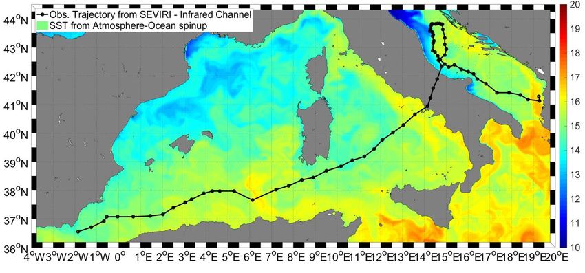
Atmosphere 2019, 10, 202                                                                              2 of 22

Occasionally, some Mediterranean cyclones may exhibit tropical-like features in their mature stage,
such as a barotropic structure, the presence of a warm core in the center of the storm with structured
and spiral convection around it, and sustained winds over 100 km/h [3–9]. Due to their resemblance to
tropical cyclones, they are usually called “medicanes” (MEDIterranean hurriCANES; [10]) or MTLCs
(Mediterranean tropical-like cyclones, [11]). Several studies have demonstrated that these systems,
which usually originate from a baroclinic wave, can transition into barotropic structures when certain
environmental conditions are met [12].
      Due to the evolution of NWP (numerical weather prediction) models, it has become possible to
study these phenomena in detail by simulating their fine horizontal and vertical structure, a feature
that is hardly resolved by satellite or in-situ observations, also considering these cyclones spend most
of their lifetime over the sea. However, despite the scientific efforts emerging in a variety of sensitivity
studies, even now NWP models suffer from a significant forecast skill reduction in the simulation of
MTLCs, as they sometimes intensify the cyclone in an unrealistic way, or fail to foresee its development
and evolution accurately. This predictability limitation depends on many factors and varies from case
to case [13]. In some events, a large sensitivity to the location of the model domain and to the horizontal
grid resolution [14] is observed, while in other cases parameterization schemes play a fundamental
role [15–17].
      Other studies (e.g., [15,18]) have shown that the large scale forcing at the initial time is the main
factor of uncertainty in the numerical simulations of medicanes.
      Generally, an important role is also played by the lateral and lower boundaries, such as the SST
field [19,20] the accuracy of which is fundamental for a realistic simulation of these cyclones [16]. Thus,
coupled ocean–atmosphere modeling systems have generally emerged as useful in order to improve
the simulation skill [21,22] via a better representation of the air–sea interaction processes.
      Some of these studies have analyzed independently the ability of a multi-physics ensemble and
of a coupled atmosphere–ocean model to simulate MTLCs; however, none have studied the two
implementations comparatively, in order to identify which one is more beneficial in terms of model
skill. This point is important for an operational center, considering that computational resources are
not infinite. For this reason, in this study, we investigate which one of the two approaches is better
suited to reproduce the evolution of an MTLC. As a case study, we choose the MTLC that occurred
in January 2014 [6]. Since this system spent most of its life cycle over the sea, it represents an ideal
case to assess the effects of air–sea interactions. In this effort, simulations with a growing level of
complexity in the representation of the SST field are considered here, also in order to better understand
its influence on the model simulations.
      The MTLC developed in the early morning of 19 January 2014 in the Alboran Sea due to a
baroclinic wave extending from the Atlantic to the Mediterranean. In the following hours, the cyclone
deepened down to a pressure minimum of 990 hPa, causing sustained wind speeds up to 100 km/h
recorded in Gibraltar airport [6]. Between the morning of 19 January 2014 and the late afternoon of
20 January 2014, the system moved across the Western Mediterranean, eventually making landfall
near Napoli (Southern Italy) at around 16 UTC. The cyclone then moved northward for about 300 km,
crossing the Apennines mountain range, and intensified again after reaching the Adriatic Sea. In the
following hours, its track rotated counterclockwise, approaching the Italian coasts; in this phase, the
cyclone intensified very rapidly, showing tropical-like features once again [6]; finally, it vanished over
the coasts of Albania (Figure 1).
      In the first group of simulations, we employed a multi-physics ensemble implementing different
microphysics and boundary layer schemes. For the setup that produces the most realistic simulation,
we modified the SST dataset, in order to evaluate the effect of a finer horizontal resolution; we also used
a uniform SST over the whole domain (using the average value), with the aim of evaluating the effect
of SST gradients. The second group of simulations was performed with the coupled atmosphere–ocean
modeling system, analyzing also the effect of the coupling timestep. Finally, an analysis of the
computational resources required for these two types of runs was performed.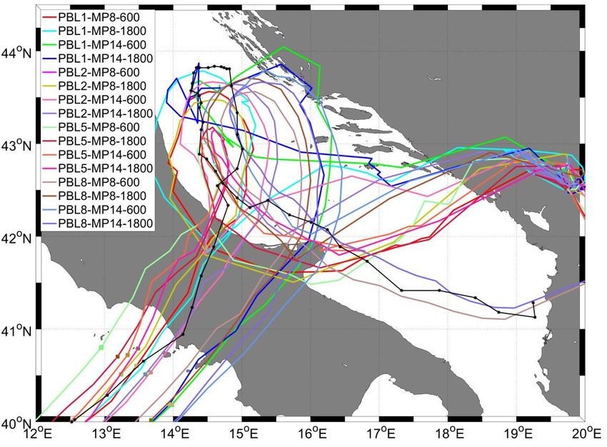
Atmosphere 2019, 10, 202 3 of 22
In Section 2, the numerical approach and the COAWST model are described in detail. Results are
discussed in Section
Atmosphere 2018, 9, x3;FOR
conclusions are drawn in Section 4.
PEER REVIEW 3 of 23
a)
Ancona
+e d
+
Ortona
Napoli
+c
c°
b
18:30Z 19/01/2014 14:45Z 20/01/2014
b) c)
L
L
21:30Z 20/01/2014 16:30Z 21/01/2014
d) e)
L
L
Figure 1. Observed
Figure trajectory
1. Observed (a) and
trajectory (a) satellite infrared
and satellite imagery
infrared at different
imagery timestimes
at different (b–e).(b–e).
The cyclone
The cyclone
trajectory was derived using 5 min rapid-scan infrared SEVIRI satellite imagery by manually identifying
trajectory was derived using 5 min rapid-scan infrared SEVIRI satellite imagery by manually
the position of the cyclone.
identifying the position of the cyclone.
2. Methods
2. Methods
2.1. COAWST Model
2.1. COAWST Model
The COAWST model (coupled ocean–atmosphere wave sediment transport; [22–26] is a numerical
framework Thethat
COAWST model coupling
entails various (coupled methods
ocean–atmosphere
among thewave sediment
atmospheric transport;
model [22–26] is a
WRF (weather
numerical
research framework
and forecasting; thatthe
[27]), entails
oceanicvarious
modelcoupling methodsocean
ROMS (regional among the atmospheric
modeling model
system; [28]), andWRF
(weather research and forecasting; [27]), the oceanic model ROMS (regional
the sediment model CSTM (community sediment transport model; [29]). In the latest version, COAWST ocean modeling system;
[28]), the
also offers andpossibility
the sediment model between
of choosing CSTM (community
the WWIII modelsediment
(wave transport
watch 3)model;
and the[29]).
SWAN Inmodel
the latest
(simulating waves in nearshore) to simulate the evolution of surface waves. The coupling amongwatch
version, COAWST also offers the possibility of choosing between the WWIII model (wave the 3)
and the SWAN model (simulating waves in nearshore) to simulate the evolution
models is obtained through the exchange of prognostic fields and is managed by the MCT libraries of surface waves.
Thecoupling
(model coupling among
toolkit; the models
[24,30,31]). is obtained
In detail, through the exchange
in the implementation used in this ofwork,
prognostic
the WRF fields
modeland is
managed by the MCT libraries (model coupling toolkit; [24,30,31]). In detail,
provided (Figure 2) the ROMS model with the heat and the momentum fluxes and then received SST in the implementation
used
fields. in this
Thus, in thework, the configuration,
coupled WRF model providedthe ROMS (Figure
model2)did thenot
ROMS model
calculate thewith
heat the
fluxesheat and the
again,
momentum
but used fluxes and
those provided bythen
the received
WRF model SST infields.
orderThus, in the coupled
to guarantee configuration,
the full consistency the ROMSthe
between model
did not
two models. calculate the heat fluxes again, but used those provided by the WRF model in order to
guarantee the full consistency between the two models.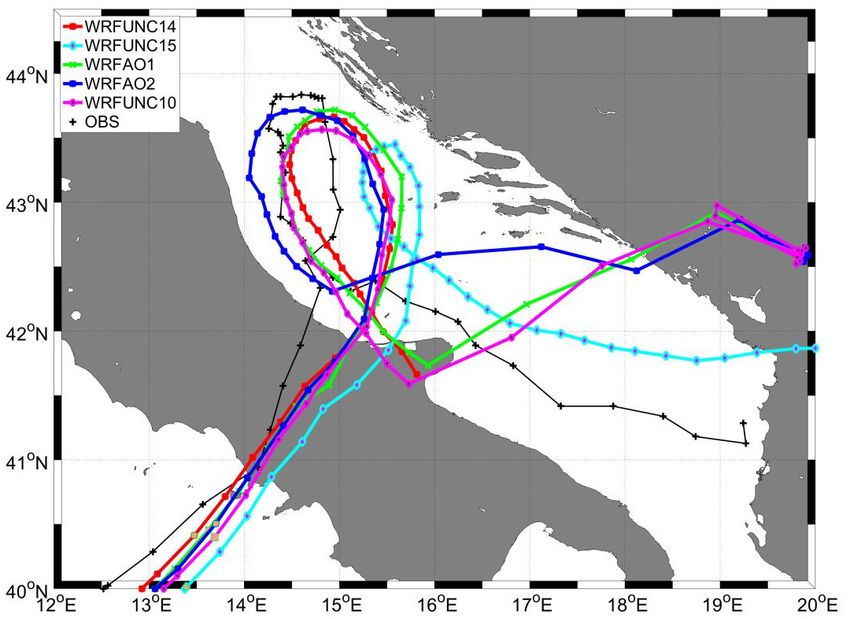
Atmosphere 2018, 9, x FOR PEER REVIEW 4 of 23
Atmosphere 2019, 10, 202 4 of 22
Figure 2. Sketch of different model configurations: (a) uncoupled approach where the sea surface
Figuretemperature
2. Sketch of (SST),
different modelevery
updated configurations:
hour, is used (a)asuncoupled approachinwhere
a lower boundary the (weather
the WRF sea surface
research and
temperature (SST), updated every hour, is used as a lower boundary in the WRF (weather
forecasting) model; (b) coupled approach with ocean and atmosphere models exchanging energy and research
and forecasting)
momentum model;
fluxes(b)(data
coupled approach
exchange maywith
occurocean and atmosphere
at different models
intervals, exchanging
i.e., every 600 s andenergy
1800 s).
and momentum fluxes (data exchange may occur at different intervals, i.e., every 600 s and 1800 s).
The COAWST model allows the coupling of the models either on the same grid or on different
The COAWST
ones. As shown model allows3,the
in Figure thecoupling
WRF domain of the configuration
models either used on theinsame grid orison
this work different
based on three grids
ones. one-way
As shownnested
in Figure
into3,each
the WRF
otherdomain
(Figureconfiguration
3), characterizedusedby in 27
thiskm work is based
(D01), 9 kmon threeand
(D02), grids
3 km (D03)
one-way nested into each other (Figure 3), characterized by 27 km (D01), 9 km (D02),
horizontal spacing. The inner domain has 925 × 563 horizontal grid points, with 60 vertical levels, and 3 km (D03)
horizontal spacing.
with deep The innerexplicitly
convection domain has 925 × 563
resolved. Thehorizontal gridlevel
first vertical points, with
is at the60 vertical
height levels,
of 12 m above the
with deep convection explicitly resolved. The first vertical level is
ground. The microphysics scheme in the coupled runs was WDM5 (WRF Double-Moment at the height of 12 m above the 5-class
ground. The microphysics
scheme), scheme
based [32], while, inin the coupled
order runs was
to parameterize theWDM5
planetary (WRF Double-Moment
boundary layer (PBL),5-class
the approach
scheme), based [32], while, in order to parameterize the planetary boundary layer (PBL), the
of [33] was used. As a shortwave radiation scheme, we used RRTMG (Rapid Radiative Transfer
approach of [33] was used. As a shortwave radiation scheme, we used RRTMG (Rapid Radiative
Model; [34]), and for the longwave we used methods used by [35]. In D01 and D02, the Kain-Fritsch
Transfer Model; [34]), and for the longwave we used methods used by [35]. In D01 and D02, the Kain-
(KF) cumulus parameterization was used. Following [6], the simulation was initialized at 00UTC,
Fritsch (KF) cumulus parameterization was used. Following [6], the simulation was initialized at
19 January 2014, using the GFS-FNL (GFS final reanalysis) dataset as initial/boundary conditions for
00UTC, 19 January 2014, using the GFS-FNL (GFS final reanalysis) dataset as initial/boundary
D01. The simulation in D03 was forced with the output fields in D02 with an hourly frequency; the
conditions for D01. The simulation in D03 was forced with the output fields in D02 with an hourly
integration timestep was 15 s. The topography had a resolution of 30”, with land-surface parameters
frequency; the integration timestep was 15 s. The topography had a resolution of 30’’, with land-
surfacetaken from thetaken
parameters MODISfromdataset.
the MODIS dataset.
As demonstrated
As demonstrated in [6], in
the[6],
SSTthe SST boundary
lower lower boundary field is for
field is critical critical for the simulation
the simulation of cycloneof cyclone
intensity and trajectory. Therefore, we decided to use the SST fields generated by a coupledcoupled
intensity and trajectory. Therefore, we decided to use the SST fields generated by a run afterrun after a
a longlong spin-up.
spin-up. Atmospheric
Atmospheric simulations
simulations werewere forced
forced withwith boundary
boundary and and initial
initial conditions
conditions takentaken from
the same dataset used for the “final” simulation (GFS-FNL). Two-way
from the same dataset used for the “final” simulation (GFS-FNL). Two-way coupled atmospheric- coupled atmospheric-ocean
oceanruns
runs were
were performed
performed for for3535days,
days,restarting
restarting thethe simulations
simulations everyevery
72 h.72After
h. After the latter
the latter period, the
period,
atmosphericmodel
the atmospheric model started
started from the the reanalyses
reanalysesatatthat thattime,
time,in order
in orderto remove
to removepossible divergence of
possible
the model
divergence of thesimulations with respect
model simulations with to the reanalyses,
respect while the
to the reanalyses, ocean
while themodel
ocean took
model thetook
initial
thecondition
initial condition from the previous run output. Ocean boundary conditions were taken from the MFSreanalysis
from the previous run output. Ocean boundary conditions were taken from the MFS [36]
datasets (see Section 4). The ocean model domain was similar to that employed for the atmospheric
model, with a grid spacing of 3 km (Figure 3). The vertical discretization consisted of 30 vertical levels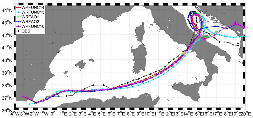
Atmosphere 2018, 9, x FOR PEER REVIEW                                                                               5 of 23
Atmosphere 2019, 10, 202                                                                                                  5 of 22
 [36] reanalysis datasets (see Section 4). The ocean model domain was similar to that employed for the
 atmospheric model, with a grid spacing of 3 km (Figure 3). The vertical discretization consisted of 30
with  increased
 vertical          resolution
          levels with           near
                        increased    the surface,
                                   resolution nearin order
                                                   the      to better
                                                       surface,        describe
                                                                in order        thedescribe
                                                                         to better   ocean mixed     layer
                                                                                              the ocean    (OML)
                                                                                                         mixed
 layer
and     (OML)
     used         and usedgenerated
            a bathymetry      a bathymetry
                                        by thegenerated  by the GEBCO
                                                GEBCO dataset,             dataset,
                                                                  characterized  by characterized
                                                                                     a 30” resolution by[37].
                                                                                                         a 30” As a
 resolution  [37].  As a mixing  scheme,  we used  the GLS  (generic length scale; [38]) approach.
mixing scheme, we used the GLS (generic length scale; [38]) approach. The ocean model initialization The ocean
 model
was       initialization
     obtained    from thewas     obtained
                            coupled        from the coupled
                                     atmosphere–ocean    spin-up atmosphere–ocean     spin-up
                                                                   described in Section   2.4. Indescribed    in
                                                                                                  this application
 Subsection
we  did not use2.4.river
                    In this application
                         input          we didinteraction
                                and sediment     not use river
                                                           withinput  and
                                                                  water    sediment interaction with water
                                                                         masses.
 masses.

 62°

                  D01
 57°

 52°                         D02

                                           D03
 47°
                                                 ROMS 3km

 42°

 37°

 32°

 27°

 22°

 17°

       47°W 42°W 37°W 32°W 27°W 22°W 17°W12°W 7°W 2°W 3°E       8°E 13°E 18°E 23°E 28°E 33°E 38°E 43°E 48°E 53°E 58°E 63°E 68°E

       Figure 3. Topography and domain configuration used for the coupled and uncoupled simulations. Red
        Figure 3. Topography and domain configuration used for the coupled and uncoupled simulations.
       lines highlight the WRF domains and the grey box delimits the ROMS model.
        Red lines highlight the WRF domains and the grey box delimits the ROMS model.
2.2. Experimental Design
 2.2. Experimental Design
      The main purpose of this work is to compare different numerical approaches for the simulation of
       The main
an MTLC.           purpose we
             In particular, of this work is
                                compare     to compare different
                                         a multi-physics            numerical
                                                             ensemble          approaches
                                                                       uncoupled    approachfor(WRFUNC)
                                                                                                the simulation
                                                                                                             with a
 of an MTLC. In particular, we compare a multi-physics ensemble uncoupled approach (WRFUNC)
coupled modeling implementation, using different coupling times (AO) (Figure 2). The comparison
 with a coupled modeling implementation, using different coupling times (AO) (Figure 2). The
is carried out in terms of cyclone trajectory, intensity, and timing. All the performed simulations are
 comparison is carried out in terms of cyclone trajectory, intensity, and timing. All the performed
summarized in Table 1. For the uncoupled simulations, we performed a comprehensive study using
 simulations are summarized in Table 1. For the uncoupled simulations, we performed a
different microphysics and PBL schemes, which, as discussed in [15], may affect both the cyclone track
 comprehensive study using different microphysics and PBL schemes, which, as discussed in [15],
and intensity. Eighteen runs, which differ for the microphysics scheme, the PBL scheme, and the type
 may affect both the cyclone track and intensity. Eighteen runs, which differ for the microphysics
of SST used, were performed. The configuration that showed the best results is used for comparison
 scheme, the PBL scheme, and the type of SST used, were performed. The configuration that showed
with  the coupled
 the best   results ismodel
                       used simulations  (Figure
                            for comparison    with2),the
                                                       in coupled
                                                          order to identify the best strategy
                                                                   model simulations          for2),operational
                                                                                        (Figure      in order touse,
considering    that  the two implementations     (multi-physics    ensemble   versus  coupled   modeling
 identify the best strategy for operational use, considering that the two implementations (multi-           system)
have   a similar
 physics          computational
           ensemble                 burden.
                       versus coupled  modeling system) have a similar computational burden.

2.3. Uncoupled   Simulations (WRFUNCP1-15)
      Table 1. List of model experiments reporting the microphysical scheme (MP), the planetary boundary
      layernumerical
     The    (PBL) scheme, andof
                      setup   the seacontrol
                                the    surface run
                                               temperature (SST) approach.
                                                   WRFUNC-CTL        (Table 1) is based on the results of [6,15].
Thus, the Thompson
           Runs        scheme for the
                                   MP parametrization   MP of microphysics
                                                                         PBL[39] and the
                                                                                      PBLMellor–Yamada–Janjic
                                                                                                     SST
     WRFUNCP-CTL
parametrization     scheme for the8 PBL [40] were    Thompson              2
                                                         used. Additionally,         MYJ         3km Spinup
                                                                                  a high-resolution   SST field,
       WRFUNCP-1                     1                 Kessler             2         MYJ
extrapolated with hourly frequency from a ROMS model run (see next section), was used. In the    3km  Spinup
       WRFUNCP-2                     2                  Lin                2         MYJ         3km Spinup
domains    D01 and D02 (Figure 3),
       WRFUNCP-3                     3 which were not  WSM3covered by the2 ROMS domain,
                                                                                     MYJ      we3km
                                                                                                  used  the SST
                                                                                                      Spinup
fields taken  from
       WRFUNCP-4    the CMEMS     dataset
                                     4      “Copernicus”
                                                       WSM5 [36], with a horizontal
                                                                           2         resolution
                                                                                     MYJ        of 6 km.
                                                                                                 3km Spinup
        WRFUNCP-5                      5                    Eta (Ferrier)            2           MYJ           3km Spinup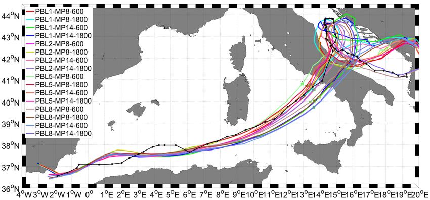
Atmosphere 2019, 10, 202                                                                               6 of 22

      Table 1. List of model experiments reporting the microphysical scheme (MP), the planetary boundary
      layer (PBL) scheme, and the sea surface temperature (SST) approach.

              Runs             MP             MP             PBL           PBL               SST
        WRFUNCP-CTL             8         Thompson             2           MYJ           3 km Spinup
          WRFUNCP-1             1           Kessler            2           MYJ           3 km Spinup
          WRFUNCP-2             2             Lin              2           MYJ           3 km Spinup
          WRFUNCP-3             3           WSM3               2           MYJ           3 km Spinup
          WRFUNCP-4             4           WSM5               2           MYJ           3 km Spinup
          WRFUNCP-5             5         Eta (Ferrier)        2           MYJ           3 km Spinup
          WRFUNCP-6             6           WSM6               2           MYJ           3 km Spinup
          WRFUNCP-7            14           WDM5               2           MYJ           3 km Spinup
          WRFUNCP-8            16           WDM6               2           MYJ           3 km Spinup
          WRFUNCP-9            14           WDM5               1           YSU           3 km Spinup
         WRFUNCP-10            14           WDM5               2           MYJ           3 km Spinup
         WRFUNCP-11            14           WDM5               4           QNSE          3 km Spinup
         WRFUNCP-12            14           WDM5               5          MYNN2          3 km Spinup
         WRFUNCP-13            14           WDM5               8          BouLac         3 km Spinup
         WRFUNCP-14            14           WDM5               2           MYJ            OML-1D
         WRFUNCP-15            14           WDM5               2           MYJ            FLAT-SST
               AO1             14           WDM5               2           MYJ            AO-1800s
               AO2             14           WDM5               2           MYJ             AO-600s

     In every uncoupled run, a slab ocean model [41] was employed, so that the initial value of SST
changed with time according to the heat fluxes, taking into account the depth of the mixed layer (50 m in
these simulations) and the lapse rate (set equal to 0.14 ◦ C/m). This approach, combined with the use of
a high-resolution initial SST, allowed us to update the SST in a way similar to the coupled runs. Starting
from this configuration, we changed the microphysics scheme as shown in Table 1 (WRFUNC1-8), and,
for the best microphysics (WDM5), we used different PBL schemes (WRFUNC-9-13). In order to test
the effect of the mixed layer depth (MLD), we changed its value from 50 to 80 m (WRFUNC-14). Finally,
to better understand the influence of the gradients of SST in the Mediterranean on the MTLC, another
simulation was performed (WRFUNC-15) using in D03 the average SST along the MTLC trajectory,
without changing the SST field in the D01-D02 domains.

2.4. Coupled Simulations (AO1-2)
    Coupled simulations used a two-way nesting configuration of WRF and ROMS models. Starting
from the configuration WRFUNC-10, which shows the best performance among the uncoupled runs,
two coupled simulations (AO1-2) were performed, and they used respectively 1800 and 600 s as
exchange times (of SST and surface fluxes) between the ocean and the atmosphere.

2.5. Ocean Spin-Up
     A long spin-up time of the oceanic model is crucial in order to reach stability in the oceanic fields
on the fine numerical grid. In order to achieve this goal, a simulation was performed over 35 days. As
discussed earlier, WRF and ROMS are two-way nested. The oceanic field at 00UTC on 19 January 2014,
at the end of the spin-up time, was used to force both the uncoupled atmospheric model simulations
(only the SST) and the coupled model (3D oceanic fields) runs.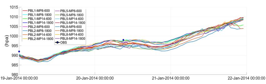
Atmosphere 2019, 10, 202                                                                          7 of 22

2.6. Data
     The analyzed event was characterized by a particularly long evolution and by a prolonged track
over the Western Mediterranean basin. With the purpose to investigate the physical characteristics
of this MTLC, we used an infrared satellite dataset. In particular, the trajectory of the cyclone was
identified using the SEVIRI data (EUMETSAT), with a frequency of 15 min. Since the MTLC moves
mostly over the open sea, the only surface data available in the central phase of its lifetime are those
over the Italian territory. We analyze sea level pressure and wind speed in the following section. The
surface stations considered here are Napoli (where the cyclone made its first landfall), Ortona, and
Ancona (both close to the track of the cyclone in the Adriatic Sea).

3. Results
     In this section, we describe the results of the multi-physics ensemble and the coupled model
simulations. First, the impact of various physical schemes and SST implementations on the MTLC
is analyzed. Next, the results of the coupled model configuration for different communication time
intervals and the comparison with the ensemble multi-physics are presented. In particular, in order to
compare the trajectory of the simulated MTLC with the observed track (Figure 1), the values of the
minimum pressure are saved together with the maximum wind intensity within a radius of 200 km
from the cyclone center. In order to quantify the distance between the simulated and the observed
trajectory, we consider purely geometrical distance (that is, independent of time) at each point of the
observed track. Lastly, we estimate the multi-physics ensemble approach compared to coupled runs in
terms of computational resources.

3.1. Microphysics Schemes
     Figure 4a shows that changes in the microphysics parametrization may affect the trajectories of
the MTLC. During its evolution, it is evident that WRFUNC1, WRFUNC3, and WRFUNC5 describe
a path of the cyclone significantly different from the observed trajectory. In particular, regarding
when the MTLC moved over the Sardinia Channel, the trajectories in WRFUNC3 and WRFUNC5
diverge compared to the observed track, remaining on its southern side for most of the transit over the
Tyrrhenian Sea. After the landfall at around 17:00 UTC, 20 January 2018 (Figure 5a), the weakening of
the cyclone made identification of the pressure minimum difficult (two weak lows can be distinguished:
one over the Southern Tyrrhenian Sea and the other inland; not shown). For the initial development
stage of the cyclone (from 9 to 36 h after the start of simulation), the three configurations produce
significant mean errors of 39, 44, and 64 km.
     In contrast, the cyclones simulated with the other five microphysical schemes remain much closer
to the observed track (Figures 4a and 5a). The small distance in Table 2 is also indicative of the good
time accuracy of the simulations, WRFUNCL7 being the best run.
     After landfall near Napoli, the MTLC moved inland and in this phase did not show tropical
characteristics [6]. The second tropical transition occurred during its transit over the Adriatic Sea
(Figure 1a), where first it moved northward and then south-southeastward. At this stage, several runs
(WRFUNC2-4-6-7-8) describe accurately the track of the cyclone (Figure 5a). However, the final part of
the cyclone is reproduced well only in WRFUNC7 (Figure 5a); in fact, the final and weakest stages in
the cyclone lifetime are generally less predictable in terms of track and minimum pressure [15].
     The time evolution of mean sea level pressure (MSLP) in Napoli (Figure 6a), Ortona (Figure 6b), and
Ancona stations (Figure 6c) shows that the evolution of the cyclone was reproduced in all simulations,
although the model responses could change by several hPa, in particular in Ortona, depending on
the large spread of the cyclone track near the Adriatic coast. About the time evolution in wind speed
in the same stations (Figure 7), the interpretation was less straightforward considering that the 10 m
wind is sensitive to small variations in the cyclone track and pressure distribution.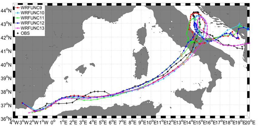
diverge compared to the observed track, remaining on its southern side for most of the transit over
the Tyrrhenian Sea. After the landfall at around 17:00 UTC, 20 January 2018 (Figure 5a), the
weakening of the cyclone made identification of the pressure minimum difficult (two weak lows can
be distinguished: one over the Southern Tyrrhenian Sea and the other inland; not shown). For the
initial development
  Atmosphere 2019, 10, 202 stage of the cyclone (from 9 to 36 h after the start of simulation), the
                                                                                                  8 ofthree
                                                                                                       22
configurations produce significant mean errors of 39, 44, and 64 km.

                                                                                                         a)

                                                                                                         b)

        Figure 4. Mediterranean tropical-like cyclone (MTLC) trajectories for the simulations using different
     Figure 4. Mediterranean tropical-like cyclone (MTLC) trajectories for the simulations using different
   Atmosphere 2018, 9, x FOR
       microphysics       (a) PEER REVIEW
                              and planetary
                                    boundary layer (PBL) schemes (b).                          8 of 23
     microphysics (a) and planetary boundary layer (PBL) schemes (b).

                                                        a)                                                          b)

        Figure    Zoom view
        Figure 5. Zoom  viewofofthe
                                 thecyclone
                                     cyclonetrajectories
                                             trajectoriesininthe
                                                               thesimulations
                                                                    simulations using
                                                                              using    different
                                                                                    different    microphysics
                                                                                              microphysics (a) (a) and
        PBL schemes
        and PBL      (b).(b).
                 schemes

        In contrast, the cyclones simulated with the other five microphysical schemes remain much
   closer to the observed track (Figures 4a and 5a). The small distance in Table 2 is also indicative of the
   good time accuracy of the simulations, WRFUNCL7 being the best run.
        After landfall near Napoli, the MTLC moved inland and in this phase did not show tropical
   characteristics [6]. The second tropical transition occurred during its transit over the Adriatic Sea
   (Figure 1a), where first it moved northward and then south-southeastward. At this stage, several runs
   (WRFUNC2-4-6-7-8) describe accurately the track of the cyclone (Figure 5a). However, the final part
   of the cyclone is reproduced well only in WRFUNC7 (Figure 5a); in fact, the final and weakest stages
   in the cyclone lifetime are generally less predictable in terms of track and minimum pressure [15].
        The time evolution of mean sea level pressure (MSLP) in Napoli (Figure 6a), Ortona (Figures 6b),
   and Ancona stations (Figures 6c) shows that the evolution of the cyclone was reproduced in all
   simulations, although the model responses could change by several hPa, in particular in Ortona,
   depending on the large spread of the cyclone track near the Adriatic coast. About the time evolution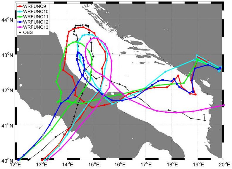
Atmosphere 2019, 10, 202                                                                                                                                                    9 of 22

         Table 2. Average value of geometric distance from the observed track in the whole track (top), in the first phase (middle) and along the Adriatic Sea (bottom).

 Pbl1         Pbl1         Pbl1    Pbl1       Pbl2       Pbl2       Pbl2       Pbl2       Pbl5        Pbl5       Pbl5       Pbl5       Pbl8       Pbl8       Pbl8          Pbl5
 Mp8          Mp8          Mp14    Mp14       Mp8        Mp8        Mp14       Mp14       Mp8         Mp8        Mp14       Mp14       Mp8        Mp8        Mp14          Mp14
 dt600        Dt1800       Dt600   Dt1800     Dt600      Dt1800     Dt600      Dt1800     Dt600       Dt1800     Dt600      Dt1800     Dt600      Dt1800     Dt600         Dt1800
 30.12        36.81        43.89   44.25      34.65      36.6       33.9       35.2       47.4        37.5       38.8       37.7       31.7       39.9       47.9          38.01
 26.84        27.49        46.24   45         27         27.13      28.8       27.7       32.41       26.79      25.97      27.1       35.22      39.22      49.31         47.7
 27.6         33.33        40.22   41.02      31.28      31         30.8       31.5       45          35.28      36.43      35.25      32         35.9       44.6          38.5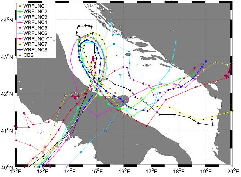
Atmosphere  2018,10,
 Atmosphere2019,  9, x202
                       FOR PEER REVIEW                                                                  1010
                                                                                                           ofof2322

     Figure 6. Comparison between the mean sea level pressure (MSLP) at Napoli, Ortona, and Ancona
     weather stations and the MSLP generated by numerical simulations. (a–c) data with different
      Figure 6. Comparison between the mean sea level pressure (MSLP) at Napoli, Ortona, and Ancona
     microphysics schemes; (d–f) data with PBL parameterizations. The blue lines indicate the landfall time
      weather stations and the MSLP generated by numerical simulations. (a–c) data with different
     over the Napoli station (a–d) and the time when the cyclone arrives close to the other stations, Ortona
      microphysics schemes; (d–f) data with PBL parameterizations. The blue lines indicate the landfall
     and Ancona.
Atmosphere 2018, 9, x FOR PEER REVIEW 11 of 23
time
Atmosphere over
2019, 10,the
202Napoli station (a–d) and the time when the cyclone arrives close to the other stations, 11 of 22
Ortona and Ancona.
Figure 7. As in Figure
Figure 6 but
7. As for the 6wind
in Figure speed
but for the for
windallspeed
uncoupled
for allsimulations. (a–c) data with different
uncoupled simulations.
microphysics schemes; (d–f) data with PBL parameterizations. The blue lines indicate the landfall time
over the Napoli station (a–d) and the time when the cyclone arrives close to the other stations, Ortona
and Ancona.Atmosphere 2019, 10, 202 12 of 22
The minimum pressure in the center of the cyclone and the maximum wind intensity nearby,
calculated along the track, are shown in Figure 8. The simulated data are comparable with the
observations in the points highlighted in blue, which represent respectively the surface station data
near the Strait of Gibraltar and in Napoli. In general, the model simulations overestimate the pressure
drop at the center of the cyclone by a few hPa, thus producing greater pressure gradients and
overestimating the wind speed on average by some m/s, which is a known general problem of
Atmosphere 2018, 9, x FOR PEER REVIEW
WRF
12 of 23
model simulations [42].
Figure
Figure 8. (Panelsa–b
8. Panels representthe
a,b)represent theMSLP
MSLPand
andmaximum
maximumwind
wind speed
speed inin the
the cyclone
cyclone center
center in uncoupled
in uncoupled
runs, c,d) the MSLP and wind speed comparison for coupled
runs, panels c–d show the MSLP and wind speed comparison for coupled runs, in a radius of 200
(panels show runs, in a radius of 200 km
km
around the cyclone along the track. Blue dots represent the value in terms of MSLP and wind
around the cyclone along the track. Blue dots represent the value in terms of MSLP and wind speed, speed,
respectively, in the early stage of cyclone and during the landfall in Napoli.
respectively, in the early stage of cyclone and during the landfall in Napoli.
To summarize the results in this subsection, we analyzed several simulations performed with
3.3. Role of SST and Coupled Simulation
different microphysics. This sensitivity approach may give different results from case to case: for
During
example, thethe genesis
MTLC of the MTLC,
studied the western
in Miglietta et al., Mediterranean
2015, shows betterSea shows an averagewith
performances positive SST
the [39]
anomaly of around
microphysics scheme0.2 °C, compared toon
(WRFUNC-CTL); climatology data [22],
the other hand, fromfor1980 to case
their 2010suggest
(from GOS-CNR Rome);
a weak sensitivity
however,
to in the Adriatic
the microphysics. Sea,
In the the anomaly
present study, allis microphysical
up to 1.8 °C (Figure
schemes 2).overestimate
The large difference in SST
the intensity of
between
the these
cyclone; two basins
however, and the strong gradient
the double-moment of SSTschemes
microphysical in the Adriatic Sea, in the
(in particular, particular
WDM5near the
scheme
Italian
with coast,
five in the
classes same area where
of hydrometeors) the to
seem TLC intensifies
achieve better(see Figure
results when1a) compared
suggested tothat the the effect
single-moment
of SST on the dynamics of this event should be investigated. In the first part of the TLC path, the
simulation WRFUNC14 (an OML with an MLD of 80 m over the entire basin) reproduces a trajectory
close to the observed path, with an average geometrical distance of 28 km, and a higher accuracy in
the first stage (25 km) compared to the second stage (30 km).
Compared to the WRFUNC10 run (an OML with an MLD of 50 m), the track in the WRFUNC14Atmosphere 2019, 10, 202 13 of 22
schemes. In particular, the run using the WDM5 microphysics better reproduces the circular path that
the cyclone took over the Adriatic Sea, especially in the northern part of the track and along the North
Adriatic coast, when the MTLC moved along an intense gradient of SSTs (see later). Finally, the use of
different microphysical schemes affects the calculation time by about 30%, from the fastest scheme
from Lin et al. to the most computational demanding WDM6 scheme.
3.2. PBL Schemes
Observing the trajectory followed by runs with different PBL schemes (Figure 4b), one can see
that, in the first part of the event, when the MTLC moves over the western Mediterranean sea, the
differences among the simulated paths and the observed trajectory increase with the time spent over
the sea (as in [22]). This suggests that the interaction between the PBL and the sea surface needs some
time to settle before influencing higher levels; in fact, in this tropical-like cyclone (TLC) phase (from 1
to 36 h), all simulations show a similar path with geometric distances from the observed track ranging
on average between 26 and 30 km. However, before landfall the WRFUNC11 (QNSE scheme, [43])
and the WRFUNC12 runs (MYNN2 scheme, [44]) generate a northward shift of about 110 and 150 km,
compare to observations.
In the second phase of the MTLC (from the 36th to the 70th h), over the Adriatic Sea, the track in
the WRFUNC11 run remains west of the other runs, closer to the Adriatic coast of Italy, where it makes
a second (erroneous) landfall at latitude 43◦ N. Similarly, the WRFUNC9 produces a wide trajectory
along the Adriatic, keeping close to the observed track, but it still makes an erroneous landfall over the
Adriatic coast of Italy. The shape of the track in WRFUNC10 and WRFUNC13 simulations remains
very close to the observed trajectory, as both produce a circle over the sea similar to the observed
trajectory. In the final part of the trajectory, the BouLac scheme (WRFUNC13) represents the path of
the cyclone much better, with a smaller geometrical distance (around 31 km). However, this is not
considered as the “reference” PBL scheme because, in this phase, the depression is weaker and does
not show the tropical features we are interested in.
The simulations WRFUNC10 and WRFUNC13 also show a more realistic intensity in the two
Adriatic stations (Ancona and Ortona), with a bias of about 2 hPa compared to the other schemes,
which overestimate the cyclone depth by about 5 hPa (Figure 6). Similar results are obtained in the
timeseries in Figure 8, where the WRFUNC11 and WRFUNC12 runs overestimate the pressure depth
by several hPa.
As shown in [45], the physical processes in the PBL drive energy exchanges at the interface with
the sea, and these exchanges influence the evolution of the atmospheric phenomena at a synoptic
level. Not surprisingly, we found a strong sensitivity to PBL schemes: as for the microphysics, the PBL
schemes that develop a northward-shift in the trajectories move the cyclone closer to the Adriatic coast,
so that it loses energy earlier due to landfall, and weakens in the Italian hinterland. As a consequence,
as shown in Figure 6, the intensity of the cyclone diverges among the various runs more significantly
after landfall. Finally, the PBL scheme marginally influences the computational times. For example the
MYJ scheme (WRFUNC10) is 8% slower than other parameterizations.
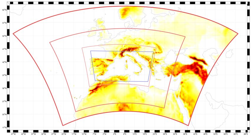
3.3. Role of SST and Coupled Simulation
During the genesis of the MTLC, the western Mediterranean Sea shows an average positive SST
anomaly of around 0.2 ◦ C, compared to climatology data from 1980 to 2010 (from GOS-CNR Rome);
however, in the Adriatic Sea, the anomaly is up to 1.8 ◦ C (Figure 2). The large difference in SST between
these two basins and the strong gradient of SST in the Adriatic Sea, in particular near the Italian coast,
in the same area where the TLC intensifies (see Figure 1a) suggested that the the effect of SST on
the dynamics of this event should be investigated. In the first part of the TLC path, the simulation
WRFUNC14 (an OML with an MLD of 80 m over the entire basin) reproduces a trajectory close to the
observed path, with an average geometrical distance of 28 km, and a higher accuracy in the first stage
(25 km) compared to the second stage (30 km).Atmosphere 2019, 10, 202 14 of 22
Compared to the WRFUNC10 run (an OML with an MLD of 50 m), the track in the WRFUNC14
simulation (an MLD of 80 m) is very close (Figure 9), while some discrepancies occur in the pressure
minimum, which is about 2 hPa deeper (and farther from the observations) at landfall near Napoli
(Figure 10a). This is probably caused by the stronger heat fluxes and greater energy available for
convection, due to the deeper mixed layer (Figure 11c). Overall, during the transit of the cyclone over
the Adriatic Sea, the differences with respect to WRFUNC10 appear small (Figures 9–11).
The run WRFUNC15 uses a uniform SST of approximately 16.6 ◦ C in the whole domain (average
value encountered by the cyclone along its track). The trajectory of this run is comparable with those
produced by the other simulations in the first stage of the TLC, with the landfall shifted southward
by about 30 km and with an average distance from the observed track of 42 km in the first stage and
60 km in the second, respectively. In the second part, the track is shifted to the east and describes a
narrower circle (Figure 9). The intensity of the storm is comparable with the other simulations during
the first 15–18 h; however, after moving for about 10 h over the Mediterranean Sea, the cyclone rapidly
intensifies, becoming 4 hPa deeper than the other runs (Figures 10a and 11a). During the transit over
the Adriatic Sea, the cyclone does not weaken, differently from the other simulations, and the pressure
minimum becomes 13 hPa deeper at the end of the simulation (Figure 11a). This is due to the fact that
the Adriatic Sea is colder than the Tyrrhenian Sea; thus, in WRFUNC15 the temperature is higher than
Atmosphere
the real value,2018,
and 9, xfluxes
FOR PEER
areREVIEW
more intense (Figure 11c). 14 of 23
a)
b)
Figure 9. MTLC
Figure simulated
9. MTLC trajectories
simulated trajectoriesover
overthe full domain
the full domain(a)(a)and
and zoom
zoom over
over the the
last last
part part
of theoftrack
the track
(b) in(b)
the simulations WRFUNC14-15, AO1, AO2, and, for the sake of comparison,
in the simulations WRFUNC14-15, AO1, AO2, and, for the sake of comparison, WRFUNC10. WRFUNC10.Atmosphere 2019, 10, 202 15 of 22
Atmosphere 2018, 9, x FOR PEER REVIEW 15 of 23
Figure 10. Observed and simulated MSLP (a–c) and wind speed (e–g) in Napoli, Ortona, and Ancona
weather stations (WRFUNC10-14-15, AO1, and AO2 runs). The blue lines indicate the landfall time
near the Napoli station (a–d) and the time when the cyclone arrives near the other stations, Ortona
and Ancona.Figure 10. Observed and simulated MSLP (a–c) and wind speed (e–g) in Napoli, Ortona, and Ancona
weather stations (WRFUNC10-14-15, AO1, and AO2 runs). The blue lines indicate the landfall time
near the Napoli station (a–d) and the time when the cyclone arrives near the other stations, Ortona
and Ancona.
Atmosphere 2019, 10, 202 16 of 22
Figure 11. MSLP in the cyclone center (panel a) and maximum wind speed (panel b) and heat fluxes
(panel c) in a radius of 200 km around the cyclone. Blue dots represent the MSLP and wind speed
Figure 11. MSLP in the cyclone center (panel a) and maximum wind speed (panel b) and heat fluxes
observed in the early stage of cyclone and during the landfall in Napoli, respectively. In panel (c), the
(panel c) in a radius of 200 km around the cyclone. Blue dots represent the MSLP and wind speed
mean heat fluxes over the same area (with a radius of 200 km around the center) are shown.
observed in the early stage of cyclone and during the landfall in Napoli, respectively. In panel (c), the
mean heat fluxes over the same area (with a radius of 200 km around the center) are shown.
The trajectories of the atmosphere–ocean coupled runs AO1 and AO2 are shown in Figure 9.
The
3.4.run AO1 isAnalysis
Sensitivity characterized by an
of the Coupled exchange time interval of 1800 s. This simulation generates the
Simulations
trajectory closest to that observed (Figure 9) among all runs (coupled and uncoupled). The distance
The goal of the present section is to disentangle the effect of coupling, that of the
between the estimated
parameterization schemes,andandsimulated trajectory
that of the coupling remains
exchange small
time on forthe
the entire cyclone
simulation lifetime, apart
of the MTLC.
from the last astage
We consider set of (Figure 9 and simulations,
coupled model Table 2). Additionally,
differing between the oceanic
landfallandtakes place a few
atmospheric kilometers
models
away from
in terms thePBL,
of the observed location
microphysics, and(Figure 9). Temporal
communication evolution
time (DT). For theand
PBL,intensity
we used YSUare (Yonsei
also consistent
with measurements,
University), apart from a small MYNN
MYJ (Mellor-Yamada-Janjic), overestimation of the cyclone intensity and
(Mellor-Yamada-Nakanishi-Niino), (Figure
BouLac10). Along
(Bougeault-Lacarrère), already considered in the uncoupled runs. For the microphysics,
the cyclone track, the minimum pressure is about 2 hPa deeper than the two available observations we focused
on the 11a),
(Figure two schemes
while thethatwind
are computationally
intensity near more efficient,center
the cyclone i.e., WDM5 (WRFoverestimated.
is slightly double moment five-
classThe
microphysics) and the [39] scheme. The chosen integration
AO2 coupled simulation uses an exchange time interval of 600 s. Its timesteps are 1800 s (consistent with
track is very similar to
the approach previously adopted in the coupled runs) and 600 s.
the AO1 run, in particular in the first phase, while later it moves closer to the Adriatic coast of Italy
Table 2 shows how the geometrical distance varies among the simulations. The change in the
(Figure 9); additionally, AO2 better reproduces the intensity of the cyclone near the Italian Adriatic
microphysics (MP8 and MP14) is responsible for significant variations, especially in the case of PBL1
coast. In the latter phase, in the morning of January 21, the cyclone weakens before moving very
rapidly towards the east. This weakening is probably caused by the passage of the simulated cyclone
over very cold coastal waters (Figure 1), which decrease the intensity of the sea surface fluxes that feed
the system (Figure 11c).Atmosphere 2019, 10, 202 17 of 22
Greater sea surface fluxes, like those simulated in WRFUNC14 and WRFUNC15, provide more
energy to the cyclone. However, they do not affect its intensity immediately; they require a time period
during which the cumulative effects of air–sea interaction processes become effective (as in Figure 4
in [9]). For example, as shown in Figure 11c, while the WRFUNC15 simulation generates more intense
heat fluxes than the other runs over the whole simulation length, the difference in terms of wind and
pressure fields increases significantly only near the end of the runs.
The sensitivity to SST and the analysis of the coupled simulations suggest some relevant indications
for hindcast and forecast applications. We found that the use of the 1D OML model, when it starts from
a high-resolution SST field similar to that employed in the initial conditions of the coupled runs, allows
for an overall good estimate of the physical and dynamical characteristics of the cyclone, although
the depth of the OML affects the results. The latter point is apparent in particular in the Adriatic Sea,
which is a semi-enclosed basin with a complex oceanic circulation and intense horizontal thermal
gradients of SST [46].
3.4. Sensitivity Analysis of the Coupled Simulations
The goal of the present section is to disentangle the effect of coupling, that of the parameterization
schemes, and that of the coupling exchange time on the simulation of the MTLC. We consider a set of
coupled model simulations, differing between oceanic and atmospheric models in terms of the PBL,
microphysics, and communication time (DT). For the PBL, we used YSU (Yonsei University), MYJ
(Mellor-Yamada-Janjic), MYNN (Mellor-Yamada-Nakanishi-Niino), and BouLac (Bougeault-Lacarrère),
already considered in the uncoupled runs. For the microphysics, we focused on the two schemes that
are computationally more efficient, i.e., WDM5 (WRF double moment five-class microphysics) and
the [39] scheme. The chosen integration timesteps are 1800 s (consistent with the approach previously
adopted in the coupled runs) and 600 s.
Table 2 shows how the geometrical distance varies among the simulations. The change in the
microphysics (MP8 and MP14) is responsible for significant variations, especially in the case of PBL1
(Figure 12). In fact, for PBL1 runs, while MP8 produces trajectories, landfalls, and time evolutions very
close to the observed data, the use of MP14 shifts the landfall to the south by almost 40 km (Figure 12).
In contrast, the effect of communication time for PBL1 runs is small. For PBL2, the simulated tracks
are all close to the observed trajectory, and the effects of microphysics and coupling time are minor
(Table 2). Lastly, the use of PBL5 or PBL8 schemes causes a shift in the trajectories, respectively, to the
north (PBL5) and to the south (PBL8) by approximately 100 km, which is compared to the observed
track (Figure 12): in these cases, the communication time has a significant effect on the model track,
especially in the second part of the simulations.
After the landfall in Napoli, one may note a rapidly growing divergence among the trajectories
(Figure 12b): the PBL1 and PBL2 schemes produce tracks closer to the observed one, PBL5 generates
trajectories shifted toward the Italian Adriatic coast and a slower evolution, and PBL8 generates
trajectories shifted to the east. Figure 13 shows a spread of almost 5 hPa among the runs in the
phase of the maximum strength of the cyclone. The simulations using the schemes PBL1 and PBL2
show the best results with a difference from observations of only 1 hPa. The choice of the timing of
communication slightly affects the development of the MTLC, which is slightly more intense for the
smallest exchange time.Atmosphere 2018, 9, x FOR PEER REVIEW 19 of 23
Atmosphere 2019, 10, 202 18 of 22
a)
b)
Figure 12. MTLC simulated trajectories over the full domain (a) and zoom of trajectories over the
Figure 12. MTLC simulated trajectories over the full domain (a) and zoom of trajectories over the last
last part
Atmosphere 2018,
ofxthe track (b) in the coupled simulations that use a different PBL, a different microphysics
part of 9,the
FOR PEER
track (b)REVIEW 20 of 23
in the coupled simulations that use a different PBL, a different microphysics
scheme, and a different coupling time.
scheme, and a different coupling time.
Figure Minimum
13.Minimum
Figure 13. MSLP MSLP versus
versus time.dots
time. Blue Blue dots represent
represent thetheMSLP
the MSLP in in theofearly
early stage stage of cyclone
cyclone
and duringthe
and during the landfall
landfall in Napoli.
in Napoli.
4. Conclusions and Remarks
In this work, we investigate in detail the impact of different factors that drive the air–sea
interaction during the numerical simulation of an MTLC. After a stand-alone atmospheric model
approach, the COAWST coupled modeling system was used, varying microphysics and planetary
boundary layer schemes and implementing the coupling between atmospheric and oceanic models
with different exchange times. The role of SST was also studied in the uncoupled simulations
considering two different OML depths (50 and 80 m) in a slab ocean model and imposing a uniformAtmosphere 2019, 10, 202 19 of 22
4. Conclusions and Remarks
In this work, we investigate in detail the impact of different factors that drive the air–sea interaction
during the numerical simulation of an MTLC. After a stand-alone atmospheric model approach, the
COAWST coupled modeling system was used, varying microphysics and planetary boundary layer
schemes and implementing the coupling between atmospheric and oceanic models with different
exchange times. The role of SST was also studied in the uncoupled simulations considering two
different OML depths (50 and 80 m) in a slab ocean model and imposing a uniform SST field over all
the ocean grid points.
The main findings emerging from the simulations can be summarized as follows:
- a sensitivity to the microphysics and boundary layer schemes was observed, which may
significantly affect the track, even more than the intensity, of the cyclone;
- the sensitivity to coupling time is limited compared to do that to physics parameterizations and
is dependent on the set of schemes considered;
- the 1D ocean model, although it suffers from limited flexibility (MLD set in the model namelist),
is able to reproduce pretty well the evolution of the cyclone, given a high-resolution initial SST
field produced by ROMS after a long spin-up time;
- air–sea interaction processes are fundamental for the proper numerical simulation of the cyclone,
and substituding the real SST with an average field may dramatically affect the intensity of
the cyclone;
- atmosphere–ocean coupled systems are the best way to take into account realistically and in a
consistent way the exchange of heat and momentum between the atmosphere and the ocean.
We can now return to the original question we posed at the beginning of the paper, i.e., whether
a multi-physics ensemble or a coupled atmosphere–ocean modeling system is ideal for simulating
Mediterranean cyclones, and from the perspective of operational use. Our conclusions are the following:
- A multi-physics ensemble, using different PBL and microphysical parameterization schemes,
produces a large spread, especially in terms of cyclone track.
- The spread of a multi-physics ensemble is too large to provide any useful information about the
detailed areas possibly affected by the cyclone, and this is probably a consequence of the fact that
some physical schemes are not specifically tuned for the Mediterranean area.
- A comprehensive study, including a large of number of cases of Mediterranean cyclones, should
be performed, in order to identify the parameterization(s) that perform better in the region for
these specific features; in search of the best configuration, one probably will not find that a certain
numerical setup is the best for all cases (Pytharoulis et al., 2018), but it is plausible that that a few
implementations will work reasonably well for all cyclones.
- After an “optimal” setup is identified, a coupled numerical simulation after a long spin up time
should provide a high-resolution SST field as a lower boundary to the atmospheric model.
- If the computational resources are sufficient, a coupled numerical simulation should be performed,
since only this strategy allows one to correctly reproduce the exchange of heat and momentum
between the ocean and the atmosphere. Although the advantage in terms of cyclone track and
intensity is limited in the present case, we reasonably expect that a great benefit in terms of the
operational prediction of wind speed, surface fluxes, and precipitation (Ricchi et al., 2016) can
be achieved.
Author Contributions: Conceptualization, A.R., G.C. and S.C.; Methodology, A.R.; Software, A.R.; Validation,
A.R., D.B., M.M.M., G.C., U.R. and S.C.; Formal Analysis, A.R., D.B., M.M.M., G.C., U.R. and S.C.; Investigation,
A.R., D.B., M.M.M., G.C., U.R. and S.C.; Resources, A.R.; Data Curation, A.R., D.B., M.M.M., G.C., U.R. and S.C.;
Writing-Original Draft Preparation, A.R., D.B., M.M.M. and S.C.; Writing-Review & Editing, A.R., D.B., M.M.M.,
G.C., U.R. and S.C.; Visualization, A.R., D.B.; Supervision, A.R. and S.C.; Project Administration, S.C.; Funding
Acquisition, S.C.Atmosphere 2019, 10, 202 20 of 22
Funding: This work was supported by RITMARE National Flagship initiative funded by the Italian Ministry
ofEducation, University and Research (IV Phase, Line 5, “Coastal Erosion and Vulnerability”) and by the EU
H2020 Programme (CEASELESS Project, grant agreement No. 730030).
Acknowledgments: Authors acknowledge the CINECA award under the ISCRA initiative (grant HP10C2SECI
“COMOLF”, Coupled Regional Modeling in Coastal Oceans, P.I. Antonio Ricchi) and specifically the kind
assistance of Isabella Baccarelli. The work was partially supported by the EU contract 730030 (call H2020-EO-2016,
“CEASELESS”, Coordinator A. Arcilla) and by RITMARE national flagship initiative funded by the Italian Ministry
of University and Research (IV phase, Line 5, “Coastal Erosion and Vulnerability”, P.I. Sandro Carniel).
Conflicts of Interest: The authors declare no conflict of interest.
References
1. Campins, J.; Genovés, A.; Picornell, M.A.; Jansà, A. Climatology of Mediterranean cyclones using the ERA-40
dataset. Int. J. Climatol. 2010, 31, 1596–1614. [CrossRef]
2. Buzzi, A.; Tibaldi, S. Cyclogenesis in the lee of the Alps: A case study. Q. J. R. Meteorol. Soc. 1978, 104,
271–287. [CrossRef]
3. Rasmussen, E.; Zick, C. A subsynoptic vortex over the Mediterranean with some resemblance to polar lows.
Tellus A 1987, 39A, 408–425. [CrossRef]
4. Lagouvardos, K.; Kotroni, V.; Nickovic, S.; Jovic, D.; Kallos, G.; Tremback, C.J. Observations and model
simulations of a winter sub-synoptic vortex over the central Mediterranean. Meteorol. Appl. 1999, 6, 371–383.
[CrossRef]
5. Royal Meteorological Society (Great Britain). In Meteorological Applications; Cambridge University Press:
Cambridge, UK, 2000.
6. Cioni, G.; Malguzzi, P.; Buzzi, A. Thermal structure and dynamical precursor of a Mediterranean tropical-like
cyclone. Q. J. R. Meteorol. Soc. 2016, 142, 1757–1766. [CrossRef]
7. Tous, M.; Romero, R.; Ramis, C. Surface heat fluxes influence on medicane trajectories and intensification.
Atmos. Res. 2013, 123, 400–411. [CrossRef]
8. Miglietta, M.M.; Laviola, S.; Malvaldi, A.; Conte, D.; Levizzani, V.; Price, C. Analysis of tropical-like cyclones
over the Mediterranean Sea through a combined modelling and satellite approach. Geophys. Res. Lett. 2013,
40, 2400–2405. [CrossRef]
9. Miglietta, M.M.; Rotunno, R. Development Mechanisms for Mediterranean Tropical-Like Cyclones
(Medicanes). Q. J. R. Meteorol. Soc. 2019. [CrossRef]
10. Emanuel, K. Increasing destructiveness of tropical cyclones over the past 30 years. Nature 2005. [CrossRef]
11. Cavicchia, L.; von Storch, H.; Gualdi, S. Mediterranean Tropical-Like Cyclones in Present and Future Climate.
J. Clim. 2014, 27, 7493–7501. [CrossRef]
12. Miglietta, M.M.; Cerrai, D.; Laviola, S.; Cattani, E.; Levizzani, V. Potential vorticity patterns in Mediterranean
“hurricanes”. Geophys. Res. Lett. 2017, 44, 2537–2545. [CrossRef]
13. Di Muzio, E.; Riemer, M.; Fink, A.H.; Maier-Gerber, M. Assessing the predictability of Medicanes in ECMWF
ensemble forecasts using an object-based approach. Q. J. R. Meteorol. Soc. 2019. [CrossRef]
14. Cioni, G.; Cerrai, D.; Klocke, D. Investigating the predictability of a Mediterranean tropical-like cyclone
using a storm-resolving model. Q. J. R. Meteorol. Soc. 2018, 144, 1598–1610. [CrossRef]
15. Miglietta, M.M.; Mastrangelo, D.; Conte, D. Influence of physics parameterization schemes on the simulation
of a tropical-like cyclone in the Mediterranean Sea. Atmos. Res. 2015, 153, 360–375. [CrossRef]
16. Ragone, F.; Mariotti, M.; Parodi, A.; Von Hardenberg, J.; Pasquero, C. A Climatological Study of Western
Mediterranean Medicanes in Numerical Simulations with Explicit and Parameterized Convection. Atmosphere
2018, 9, 397. [CrossRef]
17. Pytharoulis, I.; Kartsios, S.; Tegoulias, I.; Feidas, H.; Miglietta, M.; Matsangouras, I.; Karacostas, T. Sensitivity
of a Mediterranean Tropical-Like Cyclone to Physical Parameterizations. Atmosphere 2018, 9, 436. [CrossRef]
18. Davolio, S.; Miglietta, M.M.; Moscatello, A.; Pacifico, F.; Buzzi, A.; Rotunno, R. Natural Hazards and Earth
System Sciences Numerical forecast and analysis of a tropical-like cyclone in the Ionian Sea. Hazards Earth
Syst. Sci. 2009, 9, 551–562. [CrossRef]
19. Miglietta, M.M.; Moscatello, A.; Conte, D.; Mannarini, G.; Lacorata, G.; Rotunno, R. Numerical analysis of
a Mediterranean ‘hurricane’ over south-eastern Italy: Sensitivity experiments to sea surface temperature.
Atmos. Res. 2011, 101, 412–426. [CrossRef]You can also read