WEATHER SYSTEMS RELATED TO WET AND DRY EXTREMES - IRINA RUDEVA, GHYSLAINE BOSCHAT, ROSEANNA MCKAY, ACACIA PEPLER, ANDREW DOWDY, PANDORA HOPE JULY ...
←
→
Page content transcription
If your browser does not render page correctly, please read the page content below
Weather systems related to wet and dry extremes
 Irina Rudeva, Ghyslaine Boschat, Roseanna McKay, Acacia Pepler, Andrew Dowdy,
 Pandora Hope

 July 2021

Bureau Research Report - 053

WEATHER SYSTEMS RELATED TO WET AND DRY EXTREMES
WEATHER SYSTEMS RELATED TO WET AND DRY EXTREMES

       Weather systems related to wet and dry extremes

   Irina Rudeva, Ghyslaine Boschat, Roseanna McKay, Acacia Pepler, Andrew Dowdy,
                                                                    Pandora Hope

                                                                 Bureau Research Report No. 053

                                                                                              July 2021

National Library of Australia Cataloguing-in-Publication entry

Authors: Irina Rudeva, Ghyslaine Boschat, Roseanna McKay, Acacia Pepler, Andrew Dowdy, Pandora
Hope

Title: Weather systems related to wet and dry extremes

ISBN: 978-1-925738-27-8
ISSN: 2206-3366

Series: Bureau Research Report – BRR053

                                                                                                          i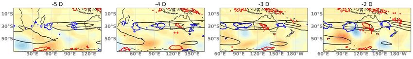
WEATHER SYSTEMS RELATED TO WET AND DRY EXTREMES

Enquiries should be addressed to:

Lead Author: Irina Rudeva

Bureau of Meteorology
GPO Box 1289, Melbourne
Victoria 3001, Australia

irina.rudeva@bom.gov.au:

Copyright and Disclaimer

     © 2021 Bureau of Meteorology. To the extent permitted by law, all rights are reserved and no part of
     this publication covered by copyright may be reproduced or copied in any form or by any means except
     with the written permission of the Bureau of Meteorology.

     The Bureau of Meteorology advise that the information contained in this publication comprises general
     statements based on scientific research. The reader is advised and needs to be aware that such
     information may be incomplete or unable to be used in any specific situation. No reliance or actions
     must therefore be made on that information without seeking prior expert professional, scientific and
     technical advice. To the extent permitted by law and the Bureau of Meteorology (including each of its
     employees and consultants) excludes all liability to any person for any consequences, including but not
     limited to all losses, damages, costs, expenses and any other compensation, arising directly or indirectly
     from using this publication (in part or in whole) and any information or material contained in it.

ii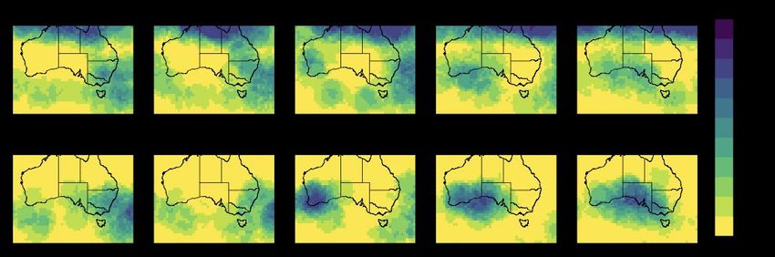
WEATHER SYSTEMS RELATED TO WET AND DRY EXTREMES

Contents
Executive Summary ................................................................................................... 1
1.     INTRODUCTION................................................................................................. 1
2.     RESULTS ........................................................................................................... 4
       2.1     Wet extremes ............................................................................................................ 4
               2.1.1         Selected cases...................................................................................................... 4
               2.1.2         Composites of weather systems ........................................................................... 6
               2.1.3         Composites of atmospheric fields during extreme events ..................................... 9
               2.1.4         Cut-off lows ......................................................................................................... 12
               2.1.5         Seasonal signature of wet extremes ................................................................... 14
       2.2     Dry events in Victoria .............................................................................................. 15
3.     Discussion ....................................................................................................... 18
4.     References....................................................................................................... 20

                                                                                                                                                    iii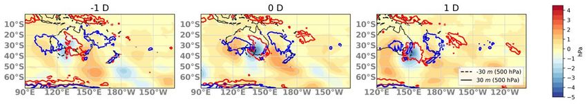
WEATHER SYSTEMS RELATED TO WET AND DRY EXTREMES
List of Figures
Figure 1: Schematic representation of (top) upper and (bottom) lower tropospheric systems and
processes leading to a cool-season extreme precipitation event in Victoria. ‘L’ and ‘H’
indicate the location of the low- and high-pressure systems, respectively, at (top) 300 hPa
and (bottom) surface .............................................................................................................. 1
Figure 2: Time series of the total Victorian JJAS and annual rainfall (based on AGCD data
[Evans et al. 2020]) and number of extreme daily rainfall events in Victoria for JJAS, during
1990-2019 .............................................................................................................................. 5
Figure 3: Composites of precipitation (mm/day) for five days centered around the selected JJAS
extreme rainfall events in Victoria .......................................................................................... 6
Figure 4: Daily composites of cyclone frequency at the 300, 500 and 700 hPa and surface levels
from 2 days prior to the extreme precipitation event in Victoria (t-2) to 2 days after the event
(t+2) ........................................................................................................................................ 7
Figure 5: Daily composites of frontal frequency defined using TFP and WND methods from 2
days prior to the extreme precipitation event in Victoria (t-2) to 2 days after the event (t+2) 8
Figure 6: As in Figure 4 but for anticyclones at (top) 500 hPa and (bottom) surface.................... 9
Figure 7: Composites of (color shading) the potential vorticity at (from top to bottom) 300, 500,
700 and 850 hPa for the period from 4 days prior to 1 day past an extreme event. Black
contours in the upper row show -2PVU [1 PVU = 10−6m−2s−1K kg−1] at four isentropic levels.
Blue and red contours show divergence and convergence ................................................. 10
Figure 8: Composites of (color shading) geopotential height anomaly at 300 hPa for the period
from 5 days prior to 1 day past an extreme event. Black contours in the zonal wind at 300
hPa. Blue (downward) and red (upward) contours show direction of vertical wind ............. 11
Figure 9: Composites of (color shading) SLP for the period from 5 days prior to 1 day past an
extreme event. Blue and red contours show divergence and convergence at 750 hPa ...... 11
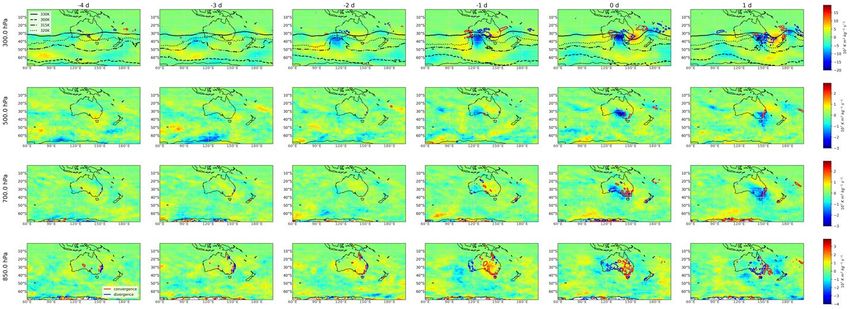
Figure 10: Composites of the integrated water vapour transport (kg m-1 s-1) for six days ending
on the day of extreme rainfall. Color shading indicate the magnitude, arrows – the direction
.............................................................................................................................................. 12
Figure 11: Composites of cut-off low frequency for three days centered on the days of extreme
rainfall in Victoria .................................................................................................................. 13
Figure 12: Count of JJAS cut-off lows at (left) any level between 290 and 350 K and (right) 300K
averaged over a region west of Victoria (35°-140°E, 40°-35°S) .......................................... 14
Figure 13: Composites of SLP anomalies from the climatological mean for (a) ’wet’ and (b) ’dry’
JJAS seasons (Pa). (c) Difference between ’wet’ and ’dry’ composites. ‘Dry’ and ‘wet’
seasons refer to the absence and presence of extreme rainfall, respectively ..................... 15
Figure 14: As in Figure 13 but for 500 hPa geopotential anomalies (m2 s-2)............................. 15
Figure 15: Duration of dry spells in JJAS defined as maximum of consecutive dry days recorded
during each cool-season (red bars) or each year (black line) over Victoria from 1980-2019.
Dry spells (CDD) are defined as days when precipitation < 1.0 mm based on ERA5 ......... 16
Figure 16: Correlation in JJAS between the CDD index calculated for Victoria (shown in Figure
12) and a) MSLP, b) 500hPa geopotential height (Z500), c) 2m air temperature and d)
precipitation anomalies in the Southern Hemisphere for the 1980-2019 period. Data is from
ERA5 reanalysis and monthly anomalies have been calculated relative to the 1979-2005
monthly climatology. Stippling indicates statistical significance at the 95% confidence level
.............................................................................................................................................. 17
iv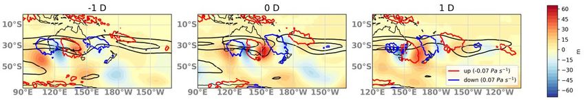
WEATHER SYSTEMS RELATED TO WET AND DRY EXTREMES

Figure 17: Length of dry spells (days) in JJAS during (a) ‘Dry’ years
    (1994,2000,2007,2008,2009,2014,2015,2017,2018), (b) ‘Wet’ years
    (1992,1993,1998,2003,2005,2013,2016) and (c) the difference between wet and dry years.
    Composite years were selected from section 2.1.5 where ‘dry’ and ‘wet’ years refer to the
    absence and presence of extreme rainfall events, respectively .......................................... 17
Figure 18: (top panel) Length of cool-season dry spells 1990-2019 (red bars; as in Figure 15 but
    focused on more recent decades) and (bottom panel) seasonal mean rainfall (blue line,
    based on AGCD data) and number of extreme rainfall events (green bars; as in Figure 2) in
    JJAS across Victoria. Note the peak in consecutive dry days in the mid-2000s aligns with a
    sequence of years with no extreme rainfall events .............................................................. 19

                                                                                                                      v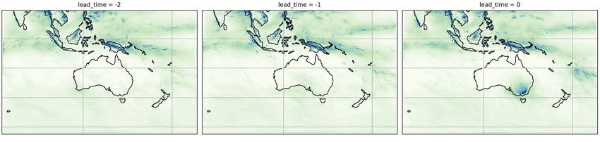
WEATHER SYSTEMS RELATED TO WET AND DRY EXTREMES

EXECUTIVE SUMMARY
The focus of this project is understanding the relationship between wet or dry cool season
(June-September) rainfall extremes in Victoria and weather systems. High rainfall
extremes, that are taken here as daily rainfall above the 99th percentile, appear to be
related to a particular combination of weather systems at various height levels through
the atmosphere. However, extremely low rainfall, associated with long lasting periods of
no rain, could not be linked as easily to fast-moving weather systems and are likely linked
to more persistent atmospheric circulation anomalies. Hence, long-lasting periods of dry
days require other approaches to understand their links to weather systems.

The evolution of high rainfall extremes starts in the upper troposphere over the
extratropical Indian Ocean 3-4 days prior to an extreme event. A Rossby wave, starting
in the Indian Ocean, propagates eastward and breaks on the day of an extreme event,
forming a cut-off low system. However, our analysis shows that not all cut-off lows
necessarily lead to extreme rainfall events. The processes leading to high synoptic rainfall
extremes are summarised in Figure 1. They include:

Figure 1: Schematic representation of (top) upper and (bottom) lower tropospheric systems and processes
leading to a cool-season extreme precipitation event in Victoria. ‘L’ and ‘H’ indicate the location of the low-
and high-pressure systems, respectively, at (top) 300 hPa and (bottom) surface

                                                                                                              1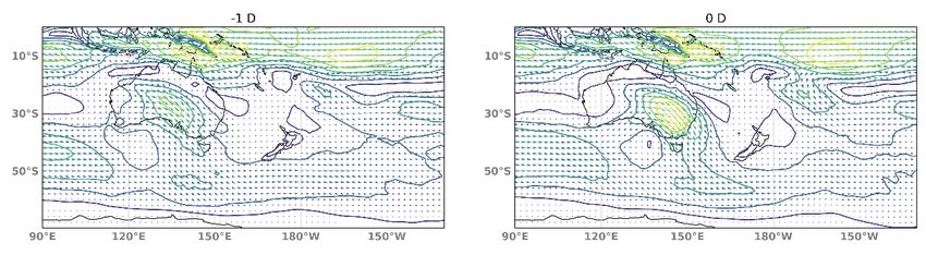
WEATHER SYSTEMS RELATED TO WET AND DRY EXTREMES

     •   An amplified Rossby wave that reaches Victoria;
     •   On the day of an extreme event an upper-level cyclone/anticyclone is located to
         the west/east of Victoria; at the low tropospheric levels, a low-pressure system is
         found over Victoria and a high-pressure system over the Tasman Sea;
     •   A Rossby wave breaking and a cut-off low to the west of Victoria;
     •   Moisture flux associated with the low-level anomalies.

The mechanisms responsible for dry spell formation are more complex and variable
compared to those leading to extreme rainfall, as dry events cannot be linked to the
passage of a particular weather type. Besides pre-conditioning (e.g., low soil-moisture)
that is known to be an important component of a drought, our analysis indicates that some
dry periods may be linked to low mean precipitation, while others can be associated with
an absence of intense rainfall events.

1.        INTRODUCTION
Understanding the physical processes associated with anomalous wet and dry rainfall can
lead to improved decision-making by policy makers and emergency services.
Preparedness for these extremes is important for a range of applications including in
agriculture, water availability and flood risk management. Many studies have examined
rainfall occurrence based on observations and modelling in Australia, with long-term
reductions in southern Australian rainfall being a common aspect of many studies
(CSIRO and BoM 2015, CCIA Technical Report; VicWaCI Synthesis Report; BoM and
CSIRO 2020 State of the Climate). However, the physical processes associated with the
decline in rainfall are not currently well-understood. Some recent studies have analysed
rainfall occurrence in relation to weather systems, including thunderstorms, cyclones and
fronts based on near-surface atmospheric conditions (Dowdy and Catto 2017; Pepler et
al. 2020), providing some insight on weather systems associated with rainfall, including
extremes in southern Australia. However, relatively few studies have focused on this in
relation to upper-level processes, even though the links between upper level and surface
systems were found to be important for heavy rainfall on the east coast of Australia
(Pepler and Dowdy 2021).

Atmospheric conditions at higher levels, in the mid- to upper-troposphere, can contribute
to rainfall occurrence, including through processes that influence the formation or
intensity of rain-bearing weather systems. These conditions include baroclinic influences
associated with frontal wave systems, mid- and upper-tropospheric vorticity and jetstream
features, Rossby wave breaking, stratospheric intrusions, atmospheric stability, nearby
high-pressure ridges or blocking systems, as well as barotropic influences associated
with convective processes and diabatic heating including latent heat release (Bjerknes
1922; Eady 1949; Lindzen and Farrel 1980; Hoskins et al. 1985; Shapiro and Keyser
1990; Hirschberg and Fritsch 1991; Bluestein 1993; Hoskins and Hodges 2002, 2005;

2
WEATHER SYSTEMS RELATED TO WET AND DRY EXTREMES
Ulbrich et al. 2009; Ndarana and Waugh 2010; Dowdy et al. 2013; Willison et al. 2013;
Catto 2016), including in relation to cyclone formation around southeast Australia
(Dowdy et al. 2019). Some of those conditions can be grouped as a common set linked
by the occurrence of upper-tropospheric advection of cyclonic vorticity, as a key forcing
mechanism for cyclone formation and associated rainfall (Godson 1948; Hirchberg and
Fritsch 1991; Dowdy et al. 2013c; da Rocha et al. 2018) together with lower values of
static stability being more conducive to deeper penetration depth of an induced circulation
(Hoskins et al. 1985; Bluestein 1993; Mills 2001). Building on such concepts, Pepler and
Dowdy (2020) recently demonstrated that the depth of cyclonic vorticity in the
troposphere is important for rainfall in southeast Australia, with deeper cyclones causing
more intense rainfall than those only identified based on near-surface conditions.
These studies highlight the benefits of considering the upper-level processes. An example
highlighting the importance of upper-level processes occurred in March 2021, when
extreme rainfall in March 2021 over the Australian east coast was observed in the absence
of a surface low along the coastline. De Vries (2021) noticed that “whereas cyclones and
warm conveyor belts, the focus of numerous studies, have a particular relevance for
precipitation and extreme precipitation in wet higher latitude regions, combined Rossby
wave breaking and intense moisture transport is very important for EPEs [extreme
precipitation events] in regions that received relatively little scientific attention, such as
the (semi)arid subtropics”. Victoria, being in the subtropics, is a hot spot for interaction
between extratropical weather systems and moisture fluxes from the tropics. In agreement
with this, a study by Holgate et al. (2020a,b) confirmed that the main source of moisture
for drought-breaking events over the Murray‐Darling Basin lies in the Coral and Tasman
Seas, but more is required to understand how this moisture source relates to upper-level
processes in the Victorian region.
The other extreme of the rainfall occurrence distribution (i.e., anomalously dry periods)
is also of interest, as it can be associated with high-pressure systems in this region (Pepler
et al 2019). Associated with this, the subtropical ridge along southern Australia is a key
mechanism leading to less rainfall than normal in this region, consisting of a series of
high-pressure systems and dry air around the descending branch of the Hadley Cell
(Drosdowsky 2005; Pepler et al. 2019; Post et al. 2014).
Here we examine aspects of upper-level processes to help improve the understanding of
the physical processes that drive extremes of rainfall in southeast Australia.
3WEATHER SYSTEMS RELATED TO WET AND DRY EXTREMES
2. RESULTS
2.1 Wet extremes
2.1.1 Selected cases
High rainfall extremes during June to September were selected using the Bureau of
Meteorology Atmospheric high-resolution Regional Reanalysis for Australia (BARRA;
Su et al. 2019) at 12 km resolution (BARRA-R). The data were interpolated onto one-
degree resolution in the Victorian area (141-150°E, 34-39°S). Days in which at least ten
grid-points in Victoria had rainfall above the 99th percentile were classed as extreme high
rainfall days. This approach helps to eliminate local rainfall anomalies caused by smaller
scale convective processes (e.g., thunderstorms). While we are interested in the influence
of synoptic-scale dynamics on rainfall extremes, using a high-resolution dataset is
important as it better reproduces the observed precipitation magnitude, compared to
reanalyses that have coarser resolution (Su et al. 2019). The analysis is done for June to
September 1990–2019.
On average, 1.22 days per season were identified as extreme rainfall events. However,
these events are not evenly distributed in time (Figure 2). In particular, the year 2016 –
the second wettest year in Victoria between 1990-2019 – had 6 extreme rainfall events,
while in 1991, the wettest JJAS in the period, there was only one event. This uneven
distribution indicates that the time series of extreme rainfall does not directly reflect the
mean or accumulative precipitation, as is the case when we talk about the wettest years
or seasons. Rather, the extreme time series reflects individual synoptic-scale rainfall
events of high intensity. Nevertheless, it is noticeable that for three consecutive cool
seasons at the end of the Millennium drought, 2007–2009, there was no extreme rainfall
events diagnosed using our metric. This is also true for years 2014–2015 and 2017–2019:
all of which are considered as dry in Victoria 1At the same time, during the first decade,
1991–2000, there was only one year with no extreme synoptic-scale rainfall events. This
is in agreement with the study by O’Donnell et al. (2021), who showed that the 20th
century was the wettest since mid-14th century, though their time series focus on the
rainfall over southwest Australia as this region is particularly well suited for studies that
use paleo proxies.
It is also interesting to note that the year 2016 is known for a strong negative phase of the
Indian Dipole (IOD), which develops during austral winter and is the most intense in
spring. Since 1990, there were 6 negative IOD years: 1992, 1996, 1998, 2010, 2014,
2016 2, with a noticeable gap in the negative IOD phase during the Millennium Drought.
All but one IOD-negative year had at least one extreme rainfall event during JJAS. On
the other hand, during the five IOD-positive years (1994, 1997, 2006, 2012, 2015), while
three years had at least one extreme rainfall event, two of the years had no events in
Victoria (1994, 2015). Some papers have suggested that the Australian climate is more
1
http://www.bom.gov.au/climate/current/statement_archives.shtml)
2
http://www.bom.gov.au/climate/iod/
4WEATHER SYSTEMS RELATED TO WET AND DRY EXTREMES
sensitive to the IOD-positive phase, which has a drying effect in south-east Australia
(Meyers et al. 2007; Cai et al. 2012, Weller and Cai 2013), however, our extreme
Victorian rainfall timeseries in Figure 2 implies that a negative phase of the IOD must be
an important driver of extreme weather, as almost all IOD-negative years coincided with
an extreme rainfall synoptic situation in Victoria.
Figure 2: Time series of the total Victorian JJAS and annual rainfall (based on AGCD data [Evans et al.
2020]) and number of extreme daily rainfall events in Victoria for JJAS, during 1990-2019
Precipitation patterns centered around extreme wet events are shown in the Figure 3. The
two days leading up to the extreme event are relatively dry. On the day of the extreme
rainfall the area-mean intensity increases to 20–30 mm/day, which is comparable to the
mean-magnitude of rainfall over the Maritime Continent. The next day, the maximum
rainfall moves further east into the Tasman Sea, suggesting that synoptic-scale extremes
are caused by midlatitude systems following the westerly flow. We note here that 20–30
mm/day may sound not very extreme because we required only 10 grid points to be above
99% percentile, meaning that the area-weighted precipitation may not be very extreme.
5WEATHER SYSTEMS RELATED TO WET AND DRY EXTREMES Figure 3: Composites of precipitation (mm/day) for five days centered around the selected JJAS extreme rainfall events in Victoria 2.1.2 Composites of weather systems We examine composites of cyclones (Figure 4) and anticyclones (Figure 6) at four levels in the troposphere: 300, 500 and 700hPa, and at sea-level, as well as surface cold-front frequency (Figure 5) during five days centered on extreme events in Figure 2 to understand the weather systems surrounding extreme rainfall events. Cyclones and anticyclones are tracked using the University of Melbourne cyclone tracking scheme (Murray and Simmonds 1991, Simmonds et al. 1999) following the approach described in Pepler and Dowdy (2020). Global 6-hourly ERA5 data at a 0.25 degree resolution are first converted to a polar stereographic grid with an effective resolution of 0.5 degrees at 30°S. Cyclones (anticyclones) are detected first as a maximum (minimum) in the Laplacian of either SLP or geopotential height, before being matched to a nearby low (high) at the corresponding level, which may be either open or closed. Cyclones at each level are required to reach a minimum Laplacian of 10 m/deg. lat.2 averaged over a 2-degree radius around the cyclone, or the equivalent intensity for cyclones identified from SLP (1.2 hPa/ deg. lat.2). To account for the larger spatial scale of anticyclones, the Laplacian is required to be below -0.075 hPa × deg. lat-2 averaged for a 10-degree radius around the anticyclone centre, and areas within a 10-degree radius of an anticyclone centre are considered to be affected by an anticyclone, consistent with anticyclone composites for Australia in Pepler et al. (2019). Cold fronts were defined using two different methods: based either on the wind shift (WND) or htermal frontal parameter (TFP). The WND method compares two consecutive 6-hour analyses of 10 m wind and identifies a front when the horizontal wind shifts in direction from the northwest to southwest quadrant and the meridional wind increases by at least 2 m s-1 over 6 hours. The other method uses a TFP, which is computed as the second derivative of the 850 hPa wet bulb potential temperature in space. The method firstly selects regions, where the TFP is above a threshold value (−5 × 10⁻¹¹ K m−2), then identifies fronts from points within these regions where the gradient of TFP is zero. See Pepler et al. (2020) for details. 6
WEATHER SYSTEMS RELATED TO WET AND DRY EXTREMES

Figure 4: Daily composites of cyclone frequency at the 300, 500 and 700 hPa and surface levels from 2 days
prior to the extreme precipitation event in Victoria (t-2) to 2 days after the event (t+2)

Figure 4 shows that at the time of an extreme rainfall over Victoria, t, a surface low to the
west of the region is found in over 40% of cases. However, the upper levels (300 and 500
hPa) show twice as high probability of a low-pressure system associated with an extreme
event (above 80%), suggesting that the upper-level atmospheric processes play a leading
role in producing rainfall extremes. The evolution of these synoptic systems shows that
they propagate from west to east at all levels. This is not the case if similar composites
are plotted for east coast extremes, particularly in the warm season, when a surface
cyclonic system often travels from the east, while an upper-level cyclone is still coming
from the west and then aligns with the lower-level system over the east coast (not shown).

                                                                                                          7
WEATHER SYSTEMS RELATED TO WET AND DRY EXTREMES Figure 5: Daily composites of frontal frequency defined using TFP and WND methods from 2 days prior to the extreme precipitation event in Victoria (t-2) to 2 days after the event (t+2) Interestingly, cold fronts (consistent across both methods used) are more frequently associated with a heavy Victorian rainfall event than surface cyclones (compare Figure 5 and the bottom row in Figure 4). Frontal frequency reach 80 %, which is similar to the frequency of upper-level lows in Figure 4 (upper row). During the two days prior to an extreme event, there is an anticyclone over south-eastern Australia and the Tasman Sea in about 30 % of cases (Figure 6), consistent with the dry weather in Victoria preceding an event (Figure 3). As this anticyclone moves further east into the Tasman Sea, it generates counterclockwise flow, which, combined with the northwesterly flow of a front approaching from the west, may contribute to the advection of moist air toward Victoria. We further explore this idea in the following section using various atmospheric parameters from ERA5. We comment here, that looking at daily composites of cyclones, anticyclones and fronts, it is becoming clear that it is not the location or intensity of the subtropical ridge nor Hadley cell extent that are causing an extreme event. These climatological features are not visible in synoptic charts and, hence, cannot be made responsible for any particular weather event, but may pre-condition the atmosphere toward fewer or more strong synoptic weather systems. A full understanding of the linkage between the longer-time average phenomenon and synoptic scales is a topic for future research. 8
WEATHER SYSTEMS RELATED TO WET AND DRY EXTREMES

Figure 6: As in Figure 4 but for anticyclones at (top) 500 hPa and (bottom) surface

2.1.3     Composites of atmospheric fields during extreme events

To explore the evolution of the extreme events, we built composites of atmospheric
variables for a few days leading up to an extreme event on day t. Figure 7 shows the
potential vorticity (PV) at the upper and lower troposphere. The strongest PV anomaly is
observed at 300 hPa. The initial perturbation is seen in the Indian Ocean as a positive
(anticyclonic) PV anomaly around 80°E, between 50° and 60°S four days before an
extreme event. The next day a negative (cyclonic) PV anomaly at 40°S – to the north of
the first positive anomaly – forms. This anomaly then moves eastward, amplifying on its
way and developing a positive PV anomaly ahead of it. On the day of extreme event this
dipole reaches Victoria, with extreme precipitation between the positive and negative PV
anomalies – and area of uplift due to strong upper-level divergence. Figure 7 is a good
illustration that upper-level processes are important for setting up the right conditions for
the development of extreme events, while the low atmospheric levels play a secondary
role showing only weak PV anomalies around the date of extreme.
Figure 7 (top row) also demonstrates that the stratosphere helps amplify the negative
tropospheric PV anomaly. The location of the dynamical tropopause is marked by -2PVU
contours at 4 isentropic levels: 300, 315, 320 and 330 K. The biggest C-shaped
perturbation of the tropopause is seen at 315 K, indicating a penetration of the
stratospheric air with lower PV than the Southern Hemisphere tropospheric air. The wave,
that first appears in the composites around 3 days before an extreme event, breaks on the
day of extreme rainfall. This is in agreement with the results by De Vries (2018), who
showed a link between a Rossby wave breaking, stratospheric intrusion and intense
moisture transport that work together to produce an extreme precipitation event.

                                                                                                           9
WEATHER SYSTEMS RELATED TO WET AND DRY EXTREMES Figure 7: Composites of (color shading) the potential vorticity at (from top to bottom) 300, 500, 700 and 850 hPa for the period from 4 days prior to 1 day past an extreme event. Black contours in the upper row show -2PVU [1 PVU = 10−6m−2s−1K kg−1] at four isentropic levels. Blue and red contours show divergence and convergence Composites of the atmospheric circulation in pressure-level coordinates reveal a weak Rossby wave (RW) pattern surrounding Antarctica prior to extreme events (seen for days 4 and 5; Figure 8). At day 4, an upper-level anticyclone (high geopotential height) at the exit region of the polar jet (~ 50°S,100°E) starts to amplify. The next day, a low-pressure system develops to the north of the anticyclone (~45°S,100°E) which is the beginning of a RW, that propagates from the midlatitudes into the subtropical area, analogous to the PV anomalies noted in Figure 7 (upper row). During its propagation, the RW intensifies, developing both upstream and downstream. Once the RW has reached the subtropical jet (STJ), west of Australia (days 3 to 2 ahead of event), it then propagates eastward along its poleward side, forming a series of low and high height anomalies along southern Australia (days 1 to 0). The resulting extreme precipitation in Victoria lies in the saddle point between low- and high-pressure anomalies located either side of the state. On the day of extreme event, the STJ is disrupted by a strong RW anomaly. We suggest here that the polar jet, seen around Antarctica to the west of 90°E, turns equatorward on day 4 and the resulting synoptic-scale propagating RW, developing on day 3, propagates along this jet. However, as we only analysed the zonal wind speed, a meridionally elongated jet may not be visible in our composites. Gillett et al. (2021) suggested that an interaction between polar and subtropical jets may be responsible for extreme events, which would be in agreement with the hypothesis above. Composites of SLP do not show noticeable anomalies until 1-2 days prior to extreme events, confirming that the upper-level dynamics play a leading role in the evolution of these events through divergence/convergence that propagate downward to the surface (Figure 9). 10
WEATHER SYSTEMS RELATED TO WET AND DRY EXTREMES

Figure 8: Composites of (color shading) geopotential height anomaly at 300 hPa for the period from 5 days
prior to 1 day past an extreme event. Black contours in the zonal wind at 300 hPa. Blue (downward) and red
(upward) contours show direction of vertical wind

Figure 9: Composites of (color shading) SLP for the period from 5 days prior to 1 day past an extreme event.
Blue and red contours show divergence and convergence at 750 hPa

Finally, the integrated water vapour transport (WVT, Figure 10) indicates that before the
development of the RW, water transports within the tropics and middle latitudes are well
separated. However, the extreme rainfall is associated with an inflow of the moisture from
the north-west. While this direction is often associated with a north-west cloud-band
(Reid et al. 2019), Figure 10b suggests that the moisture comes from a range of sources,
including the Great Australian Bight and, possibly, northern/north-eastern seas (including
the Coral Sea) to converge over central-inland Australia in the days preceding the rain
event as the Rossby wave approaches Victoria. Future research using back-trajectory
analysis will aim to explicitly identify the sources of moisture supplying extreme rainfall
events rather than inferring from instantaneous IWVT fields.

                                                                                                          11
WEATHER SYSTEMS RELATED TO WET AND DRY EXTREMES Figure 10: Composites of the integrated water vapour transport (kg m-1 s-1) for six days ending on the day of extreme rainfall. Color shading indicate the magnitude, arrows – the direction 2.1.4 Cut-off lows Upper-level circulation anomalies are often associated with a RW breaking (RWB), which leads to the formation of cut-off lows, introduced by Palmén and Newton (1969). Traditionally, cut-off lows refer to closed geopotential height contours in the middle or upper troposphere (e.g., Bell and Bosart, 1989; Nieto et al., 2005; Munoz et al., 2020) with stratospheric air in regions that are climatologically tropospheric. Stratospheric air is known for lower values of the PV, below -2 PVU in the SH, whereas tropospheric air masses typically have higher PV. Using a PV framework, Portmann at al. (2021) identified cut-offs as closed regions with PV values lower than -2 PVU on a few isentropic surfaces. While Palmén and Newton (1969) called cut-off lows upper-level closed cyclones equatorward of the jet stream, PV cut-offs identified in Portmann et al. (2021) can be found on both sides of the jet. Moreover, their analysis suggests that cut- off lows in the Australian sector during cool-season form between the subtropical and polar jets. 12
WEATHER SYSTEMS RELATED TO WET AND DRY EXTREMES

Using Portmann et al.’s dataset, we built composites of the cut-off lows for the extreme
rainfall events in Victoria (Figure 11). Cut off lows at any level between 290 and 360 K
were considered, however, Portmann et al. (2021) showed that in the Australian sector
most of the cool season cut-off are observed between 300 and 310K. As can be suggested
from Figure 7, which shows a breaking RW on day 0 to the west of Victoria, Figure 11
shows that an extreme Victorian rainfall is often associated with a cut-off low
approaching from the west, which then continues moving to the east into the Tasman Sea.
Portmann et al. (2021) showed that a large number of cut-off lows decay diabatically once
they reach the Tasman Sea.

Figure 11: Composites of cut-off low frequency for three days centered on the days of extreme rainfall in
Victoria

Based on the information in Figure 11, we calculated the number of cut-off lows in the
area of their maximum frequency on day 0 (135°-140°E, 40°-35°S) (Figure 12) at any
level in the dataset (projected over all levels between 290 and 350 K) or at 300K between
1979 to 2017. There is a high level of interannual variability in the number of cut-off lows
over this time period. Overall, there is a weak increasing trend in the total number of cut
off lows in JJAS, that may be a result of the circulation change in late 1990s (Lucas et al.
2021). However, cut-off lows at 300K, i.e., systems that penetrate deeper into the
troposphere, show a very weak (not statistically significant) downward trend.

                                                                                                        13
WEATHER SYSTEMS RELATED TO WET AND DRY EXTREMES Figure 12: Count of JJAS cut-off lows at (left) any level between 290 and 350 K and (right) 300K averaged over a region west of Victoria (35°-140°E, 40°-35°S) Interestingly, the years with the highest rainfall over the 99th percentile do not necessarily correspond to the years with significant numbers of either total or 300K cut-off low time series, shown in Figure 12. This weak (or absent) relationship suggests that there is more to understand about how cut-off lows are related to extreme rainfall. Cut off low depth through the atmosphere, intensity, and duration may be more important in inducing extreme rainfall but are not captured in a simple count. Cut-off low depth, in particular, may reflect the need for a cutoff low to correspond to a surface low feature for extreme events (Barnes et al. 2021). Albers et al. (2021) argue that the horizontal extent of the stratospheric intrusions, which accomplishes cut-off lows, is more important in developing deeper surface cyclones than the vertical depth of the stratospheric intrusion. The interaction with moisture sources, such as atmospheric rivers (e.g., Reid et al. 2020) or other weather types, such as fronts and thunderstorms (e.g., Pepler et al. 2020), may also be important. 2.1.5 Seasonal signature of wet extremes Figures 13 and 14 shows composites of seasonal mean SLP and 500 hPa geopotential height (Z500) anomalies, respectively, for years with and without the extreme rainfall anomalies in Victoria, shown in Figure 2. The strongest anomaly during years with extreme rainfall events is the strong Amundsen Sea Low (centered on 120° W). 14
WEATHER SYSTEMS RELATED TO WET AND DRY EXTREMES
Interestingly, a high-pressure anomaly in the high-latitude southern Indian Ocean is found
in the same location as 4 days before an extreme rainfall in Figure 8. This seasonal
circulation anomaly suggests that wet JJAS seasons have similar and consistent RW
propagate from this region toward Victoria, some of which generate extreme rainfall.
More broadly, the extratropics during ‘wet’ years are characterised by stronger polar jet
and amplified zonal-wave 3. In contrast, during years without extreme rainfall events,
high latitudes to the south of Australia and in the western South Pacific are characterised
by high pressure anomalies.
Over Australia, dry and wet years are associated with high- and low-pressure anomalies,
respectively. Anomalous low pressure over Australia suggests more synoptic activity
during wet years, that help advect moisture at lower levels and bring it to Victoria, as
shown in Figure 10. On the other hand, high-pressure anomaly during dry years indicates
either fewer low-pressure systems, that are important for moisture advection, or reduced
uplift. However, weaker SLP anomalies for years without extreme events may indicate a
more diverse mechanisms that cause long-lasting dry events.
Figure 13: Composites of SLP anomalies from the climatological mean for (a) ’wet’ and (b) ’dry’ JJAS
seasons (Pa). (c) Difference between ’wet’ and ’dry’ composites. ‘Dry’ and ‘wet’ seasons refer to the
absence and presence of extreme rainfall, respectively
Figure 14: As in Figure 13 but for 500 hPa geopotential anomalies (m2 s-2)
2.2 Dry events in Victoria
Dry events or spells are characterised by a period of abnormally dry weather. We examine
cool-season dry spells in Victoria by calculating the number of consecutive dry days (dry
defined as when rainfall remains below 1.0 mm) at every grid point and for each JJAS
season from 1979 to 2020. The Consecutive Dry Days (CDD) index, shown in Figure 15,
was calculated using daily precipitation data from ERA5 reanalysis (see ETCCDI indices,
Karl et al., 1999), and indicates the duration of the longest dry spells averaged over all
grid points in Victoria for each season or year.
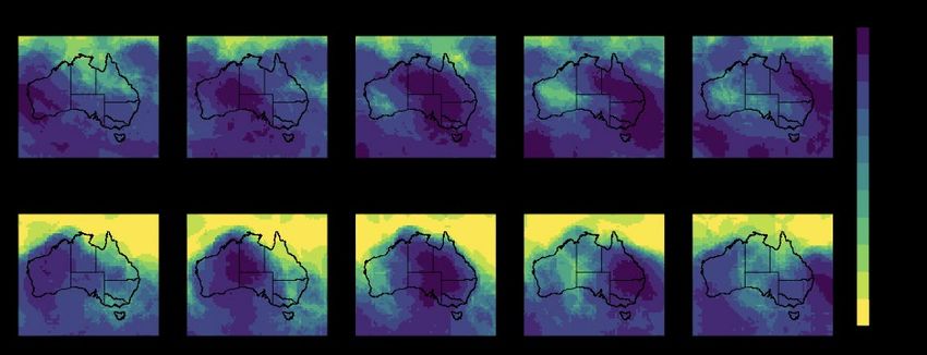
15WEATHER SYSTEMS RELATED TO WET AND DRY EXTREMES Figure 15: Duration of dry spells in JJAS defined as maximum of consecutive dry days recorded during each cool-season (red bars) or each year (black line) over Victoria from 1980-2019. Dry spells (CDD) are defined as days when precipitation < 1.0 mm based on ERA5 In the cool-season, Victoria can regionally experience dry spells that can last up to between 10 to 20 days, which is about half as long as they can last during the entire year (see black line, Figure 15). The annual CDD shows marked interannual variations, as well as periods of apparent increasing trends such as from the late 1990s to the late 2000s which coincides with the Millenium Drought. It is interesting to note that the Millennium Drought had periods of long dry spells in JJAS, particularly, in 2005-2007 (CDD>20 days), whereas during other periods, the drought was marked by an absence of extreme rainfall (as discussed in Section 2.1.1, see 2007-2009 in Figure 1). Figure 16 shows the correlation between the CDD index for Victoria (shown in Figure 15) and atmospheric pressure fields across the Southern Hemisphere for the JJAS season. This figure illustrates how dry events in Victoria are typically associated with a significant high-pressure system centred over Victoria at the surface and over the Great Australian Bight in the mid-troposphere (Figure 16a-b). Rainfall deficit (Figure 16d) has been linked to increases in surface temperature through reduced cloud cover and stronger incoming shortwave radiation (Yin et al., 2014). These higher temperatures (Figure 16c) can act together with wind speed to increase the vapour pressure deficit and evaporative demand, which causes further drying of the land and prolonged drought conditions (i.e., increase in CDD). Results from our correlation analysis also suggest a relationship between dry events in Victoria and variability in the Amundsen Sea Low region which will need to be further investigated, as well as generally higher SLP in the high latitudes, which represents a negative Southern Annular Mode pattern (SAM; the leading mode of variability in the high latitudes, e.g., see Thompson and Wallace, 2000). 16
WEATHER SYSTEMS RELATED TO WET AND DRY EXTREMES

Figure 16: Correlation in JJAS between the CDD index calculated for Victoria (shown in Figure 12) and a)
MSLP, b) 500hPa geopotential height (Z500), c) 2m air temperature and d) precipitation anomalies in the
Southern Hemisphere for the 1980-2019 period. Data is from ERA5 reanalysis and monthly anomalies
have been calculated relative to the 1979-2005 monthly climatology. Stippling indicates statistical
significance at the 95% confidence level

Dry events are more complex than the extreme high rainfall events considered in this
study as they cannot be linked to a passage of an individual weather system. In Figure 17,
we examine the length of cool-season dry spells across Victoria during years of extreme
rainfall occurrence (i.e., ‘wet years’), and compare it to years when no extreme event was
recorded (i.e., ‘dry years’) as discussed in section 2.1.5.

Figure 17: Length of dry spells (days) in JJAS during (a) ‘Dry’ years
(1994,2000,2007,2008,2009,2014,2015,2017,2018), (b) ‘Wet’ years
(1992,1993,1998,2003,2005,2013,2016) and (c) the difference between wet and dry years. Composite
years were selected from section 2.1.5 where ‘dry’ and ‘wet’ years refer to the absence and presence of
extreme rainfall events, respectively

On average, Victorian regions can experience between 5 days (near to coast) and up to a
maximum 25 days (further inland and northwest) of continuously ‘dry’ (with precipitation
below
WEATHER SYSTEMS RELATED TO WET AND DRY EXTREMES

cool-season seasons that include extreme rainfall events (‘wet’ years), which is consistent
with a north-west moisture influx shown in Figure 10b.

Along with the Standardized Precipitation Index (SPI; McKee et al; 1993), CDD is one
of the most widely used indices to analyse meteorological drought and is based only on
precipitation. However, we need to bear in mind that droughts are not only defined by a
lack of rainfall. Dry conditions can also be induced by other meteorological factors such
as potential evapotranspiration (increased by enhanced radiation, wind speed or vapor
pressure deficit) and, for example, by certain pre-conditioning of the soil, streamflow or
groundwater storage. These factors can play a key role in the duration and severity of a
drought and will need to be taken into account depending on what aspect of the drought
we are interested in studying (Seneviratne et al. 2012; Alexander et al., 2019).

3.        DISCUSSION
It is interesting to compare our results with findings by Hauser et al. (2020), who
performed an extensive analysis of winter-spring rainfall monthly anomalies. Their key
finding is that the location of high-pressure systems plays a leading role in determining a
pathway of moisture advection and is also closely linked to the presence or absence of
cut-off lows. However, one of three wet clusters, and the only dry cluster, identified by
Hauser et al., did not show any statistically significant anomaly in the frequency of cut-
off lows, which agrees with our findings. Furthermore, Hauser et al. also associated the
frequency of dry and wet clusters with ENSO anomalies and found that the dry cluster is
more often associated with El Niño anomalies; on the other hand, as 52 % of all El Niño
cool seasons were associated with wet conditions in southeastern Australia, these results
should be taken with caution as ENSO is still developing during the cool season. Findings
by Hauser et al., taken together with our findings, suggest that extreme anomalies require
a combination of weather systems and an interaction of those at different atmospheric
levels is required to produce an extreme event. In line with Hauser et al., in our future
work we will focus more on the characteristics of high-pressure systems around Victoria
and their associated RW breaking, formation of cut-off lows, and anomalous moisture
transport. Furthermore, a persistent high-pressure system may be responsible for dry
events and will be related to the formation of blocking highs.

It is interesting to note that The Millennium Drought had periods of long dry spells in
JJAS, particularly, in 2005-2007 (CDD>20 days). As discussed in Section 2.1.1, the
drought was also marked by the absence of extreme rainfall events during 2007-2009
(Figure 18). Furthermore, starting from late 1990s the number of extreme events per JJAS
better corresponds to the mean precipitation than it did in the early and mid-1990s. This
may be related to a shift in circulation patterns found around 1997 in our previous work
on the isentropic circulation (Rudeva et al. 2019). Another interesting hypothesis was
proposed by King et al. (2020), who found that recent dry years in southeastern Australia
– particularly since 2017, that are also marked by the absence of extreme rainfall events
over Victoria – were facilitated by an absence of strong IOD and ENSO events. They
speculated that more pronounced modes of these large-scale modes of variability are
responsible for the development of rain bearing systems that can terminate a drought.

18
WEATHER SYSTEMS RELATED TO WET AND DRY EXTREMES

While this hypothesis may well explain the recent dry years, it does not explain all of
them (see our discussion on the IOD years in Section 2.1.1; ENSO is less relevant during
austral cool-season).

Figure 18: (top panel) Length of cool-season dry spells 1990-2019 (red bars; as in Figure 15 but focused
on more recent decades) and (bottom panel) seasonal mean rainfall (blue line, based on AGCD data) and
number of extreme rainfall events (green bars; as in Figure 2) in JJAS across Victoria. Note the peak in
consecutive dry days in the mid-2000s aligns with a sequence of years with no extreme rainfall events

Findings of this project helped identify gaps in our understanding of the processes leading
to anomalous rainfall in Victoria. While the large-scale drivers have been recognized as
important drivers of rainfall anomalies over Australia, their role in creating synoptic
circulation anomalies is not yet understood. This will be the focus of our work in
VicWaCI2. In particular, we will be exploring links between the IOD, upper-level jets
and synoptic conditions in Victoria during winter and spring seasons. Furthermore, to
better identify the sources of moisture, we will use back-trajectory analysis instead of the
instantaneous WVF. Finally, our work will explore the role of a high-pressure system in
the Tasman Sea in creating anomalous moisture flux, bringing moisture onshore, and how
the frequency and persistence of this high is linked to large-scale drivers.

                                                                                                        19
WEATHER SYSTEMS RELATED TO WET AND DRY EXTREMES
4. REFERENCES
Albers, J. R., Butler, A. H., Breeden, M. L., Langford, A. O., and Kiladis, G. N.:
Subseasonal prediction of springtime Pacific–North American transport using
upper-level wind forecasts, Weather Clim. Dynam., 2, 433–452,
https://doi.org/10.5194/wcd-2-433-2021, 2021.
Alexander LV; Fowler HJ; Bador M; Behrangi A; Donat M; Dunn R; Funk C; Goldie J;
Lewis E; Rogé M; Seneviratne SI; Venugopal V, 2019, 'On the use of indices to
study extreme precipitation on sub-daily and daily timescales', Environmental
Research Letters, http://dx.doi.org/10.1088/1748-9326/ab51b6
Barnes, M.A., Ndarana, T. & Landman, W.A. Cut-off lows in the Southern Hemisphere
and their extension to the surface. Clim Dyn 56, 3709–3732 (2021).
https://doi.org/10.1007/s00382-021-05662-7
Bell, G. and Bosart, L.: A case-study diagnosis of the formation of an upper-level cutoff
cyclonic circulation over the eastern United States, Mon. Weather Rev., 121,
1635–1655, https://doi.org/10.1175/1520-
0493(1993)1212.0.CO;2, 1993.
Bluestein HR (1993) Synoptic-Dynamic Meteorology in Midlatitudes. Vol. II:
Observations and Theory of Weather Systems. Oxford University Press, 594 pp.
Bjerknes J (1922) Life cycle of cyclones and the polar front theory of atmospheric
circulation. Geophys. Publik., 3(1), pp.1-18.
Cai, W., van Rensch, P., Cowan, T., & Hendon, H. H. (2012). An Asymmetry in the IOD
and ENSO Teleconnection Pathway and Its Impact on Australian Climate.
Journal of Climate, 25(18), 6318–6329. https://doi.org/10.1175/JCLI-D-11-
00501.1
CSIRO and Bureau of Meteorology. Climate Change in Australia Information for
Australia's Natural Resource Management Regions: Technical Report. 2015
De Vries, A. J., Ouwersloot, H. G., Feldstein, S. B., Riemer, M., El Kenawy, A. M.,
McCabe, M. F., and Lelieveld, J.: Identification of tropical-extratropical
interactions and extreme precipitation events in the Middle East based on potential
vorticity and moisture transport, J. Geophys. Res.-Atmos., 123, 861–881, 2018.
De Vries, A. J., 2021: A global climatological perspective on the importance of Rossby
wave breaking and intense moisture transport for extreme precipitation events.
Weather Clim. Dynam., 2, 129–161. https://doi.org/10.5194/wcd-2-129-2021
Dowdy AJ, Mills GA, Timbal B (2013) Large-scale diagnostics of extratropical
cyclogenesis in eastern Australia. Int. J. Climatol., 33(10), 2318-2327.
doi:10.1002/joc.3599
20WEATHER SYSTEMS RELATED TO WET AND DRY EXTREMES
Dowdy, A.J. and Catto, J.L., 2017. Extreme weather caused by concurrent cyclone, front
and thunderstorm occurrences. Scientific reports, 7(1), pp.1-8.
Dowdy, A.J., Pepler, A., Di Luca, A., Cavicchia, L., Mills, G., Evans, J.P., Louis, S.,
McInnes, K.L. and Walsh, K., 2019. Review of Australian east coast low pressure
systems and associated extremes. Climate Dynamics, 53(7), pp.4887-4910.
Drosdowsky, W. (2005). The latitude of the subtropical ridge over Eastern Australia: The
L index revisited. International Journal of Climatology. 25. 1291 - 1299.
10.1002/joc.1196.
Eady E (1949) Long waves and cyclone waves. Tellus, 1, 33-52. doi.org/10.1111/j.2153-
3490.1949.tb01265.x.
Evans, A., D. Jones, R. Smalley, S. Lellyett, 2020: An enhanced gridded rainfall analysis
scheme for Australia. Bureau Research Report No. 041. ISBN: 978-1-925738-12-
4.
Gillett, Z. E., Hendon, H. H., Arblaster, J. M., & Lim, E.-P. (2021). Tropical and
Extratropical Influences on the Variability of the Southern Hemisphere
Wintertime Subtropical Jet, Journal of Climate, 34(10), 4009-4022.
Godson WL (1948) A new tendency equation and its application to the analysis of surface
pressure changes. Journal of Meteorology, 5(5), pp.227-235.
Hauser, S, Grams, CM, Reeder, MJ, McGregor, S, Fink, AH, Quinting, JF. A weather
system perspective on winter–spring rainfall variability in southeastern Australia
during El Niño. QJR Meteorol Soc. 2020; 146: 2614– 2633.
https://doi.org/10.1002/qj.3808
Hirschberg PA, Fritsch JM (1991) Tropopause undulations and the development of
extratropical cyclones. Part I. Overview and observations from a cyclone event.
Monthly weather review, 119(2), pp.496-517.
Holgate, C. M., Van Dijk, A. I. J. M., Evans, J. P., & Pitman, A. J. (2020a). Local and
remote drivers of southeast Australian drought. Geophysical Research Letters, 47,
e2020GL090238. https://doi.org/10.1029/2020GL090238
Holgate, C. M., Evans, J. P., van Dijk, A. I. J. M., Pitman, A. J., & Di Virgilio, G. (2020b).
Australian Precipitation Recycling and Evaporative Source Regions, Journal of
Climate, 33(20), 8721-8735. https://doi.org/10.1175/JCLI-D-19-0926.1
Hoskins BJ, McIntyre ME, Robertson AW (1985) On the use and significance of
isentropic potential vorticity maps. Quart. J. Roy. Meteor. Soc., 111, 877-946.
Hoskins BJ, Hodges KI (2002) New perspectives on the Northern Hemisphere winter
storm tracks. Journal of the Atmospheric Sciences, 59(6), pp.1041-1061.
21WEATHER SYSTEMS RELATED TO WET AND DRY EXTREMES
Hoskins BJ, Hodges KI (2005) A new perspective on Southern Hemisphere storm
tracks. Journal of Climate, 18(20), pp.4108-4129.
Karl TR, Nicholls N, Ghazi A, 1999: CLIVAR/GCOS/WMO workshop on indices and
indicators for climate extremes: workshop summary. Clim Change, 42, p.3–7.
King, A.D., Pitman, A.J., Henley, B.J. et al. The role of climate variability in Australian
drought. Nat. Clim. Chang. 10, 177–179 (2020). https://doi.org/10.1038/s41558-
020-0718-z
Lindzen RS, Farrell F (1980) A Simple Approximate Result for the Maximum Growth
Rate of Baroclinic Instabilities. J. Atmos. Sci., 37, 1648-1654.
Meyers, G., McIntosh, P., Pigot, L., & Pook, M. (2007). The Years of El Niño, La Niña,
and Interactions with the Tropical Indian Ocean. Journal of Climate, 20(13),
2872–2880. https://doi.org/10.1175/JCLI4152.1
McKee, T.B., N.J. Doesken, and J. Kleist, 1993: The relationship of drought frequency
and duration to time scales. In: Proceedings of the 8th Conference on Applied
Climatology, Anaheim, California, 17-22 Jan 1993, pp. 179-184.
Munoz, C., Schultz, D., and Vaughan, G.: A midlatitude climatology and interannual
variability of 200-and 500-hPa cut-off lows, J. Clim., 33, 2201–2222,
https://doi.org/10.1175/JCLI-D-19-0497.1, 2020.
Murray, R. J., and I. Simmonds, 1991: A numerical scheme for tracking cyclone centres
from digital data. Part I: Development and operation of the scheme. Aust. Meteor.
Mag.,39, 155–166.
Ndarana T, Waugh DW (2010) The link between cut‐off lows and Rossby wave breaking
in the Southern Hemisphere. Quarterly Journal of the Royal Meteorological
Society, 136(649), pp.869-885.
Nieto, R., Gimeno, L., de la Torre, L., Ribera, P., Gallego, D., García-Herrera, R., García,
J. A., Redaño, A., and Lorente, J.: Climatological features of cutoff low systems
in the Northern Hemisphere, J. Clim., 18, 3085–3103,
https://doi.org/10.1175/JCLI3386.1, 2005.
O’Donnell, A.J., McCaw, W.L., Cook, E.R. et al. Megadroughts and pluvials in
southwest Australia: 1350–2017 CE. Clim Dyn (2021).
https://doi.org/10.1007/s00382-021-05782-0
Palmén, E. and Newton, C. W.: Atmospheric circulation systems: their structure and
physical interpretation, New York : Academic Press, 1969.Pepler, A.S., Dowdy,
A.J., van Rensch, P., Rudeva, I., Catto, J.L. and Hope, P., 2020. The contributions
22WEATHER SYSTEMS RELATED TO WET AND DRY EXTREMES
of fronts, lows and thunderstorms to southern Australian rainfall. Climate
Dynamics, 55(5), pp.1489-1505.
Pepler, A. and Dowdy, A., 2020. A three-dimensional perspective on extratropical
cyclone impacts. Journal of Climate, 33(13), pp.5635-5649.
Pepler, A., & Dowdy, A. (2021). Intense east coast lows and associated rainfall in eastern
Australia. Journal of Southern Hemisphere Earth Systems Science, 71(1), 110–122.
https://doi.org/10.1071/ES20013
Pepler, A., P. Hope, and A. Dowdy, 2019: Long-term changes in southern Australian
anticyclones and their impacts. Clim. Dyn., 53, 4701,
https://doi.org/10.1007/s00382-019-04819-9.
Portmann, R., M. Sprenger, and H. Wernli, 2021: The three-dimensional life cycles of
potential vorticity cutoffs: a global and selected regional climatologies in ERA-
Interim (1979–2018). Weather Clim. Dynam., 2, 507–534.
https://doi.org/10.5194/wcd-2-507-2021
Reid, K. J., King, A. D., Lane, T. P., & Short, E. (2020). The sensitivity of atmospheric
river identification to integrated water vapor transport threshold, resolution, and
regridding method. Journal of Geophysical Research: Atmospheres, 125,
e2020JD032897. https://doi.org/10.1029/2020JD032897
Reid, K. J., Simmonds, I., Vincent, C. L., & King, A. D. (2019). The Australian Northwest
Cloudband: Climatology, Mechanisms, and Association with Precipitation,
Journal of Climate, 32(20), 6665-6684.
Rudeva, I., C. Lucas, B. Boschat, L. Ashcroft, P. Hope and A. Pepler, 2021: Variability
of Southern Hemisphere circulation patterns from an isentropic perspective.
Under review.
Rudeva, I., I. Simmonds, D. Crock, and G. Boschat, 2019: Midlatitude fronts and
variability in the Southern Hemisphere tropical width. J. Climate, 32, 8243–8260,
https://doi.org/10.1175/JCLI-D-18-0782.1
Shapiro MA, Keyser DA (1990) Fronts, jet streams, and the tropopause (pp. 167-191).
US Department of Commerce, National Oceanic and Atmospheric Administration
Environmental Research Laboratories, Wave Propagation Laboratory.
Seneviratne, S., and co-authors, 2012: Changes in climate extremes and their impacts on
the natural physical environment, in Managing the Risks of Extreme Events and
Disasters to Advance Climate Change Adaptation, A Special Report of Working
Groups I and II of the Intergovernmental Panel on Climate Change (IPCC), edited
by C. B. Field et al., pp. 109–230, Cambridge Univ. Press, Cambridge, U. K.
https://doi.org/10.7916/d8-6nbt-s431
23You can also read