Greenhouse Climate Optimization using Weather Forecasts and Machine Learning - Serie TVE-F Victoria Sedig Evelina Samuelsson Nils Gumaelius Andrea ...
←
→
Page content transcription
If your browser does not render page correctly, please read the page content below
19013

                      Examensarbete 15 hp
                                Juni 2019

Greenhouse Climate Optimization
using Weather Forecasts and Machine
Learning
Serie TVE-F

Victoria Sedig
Evelina Samuelsson
Nils Gumaelius
Andrea Lindgren
Populärveteskaplig sammanfattning I projektet Greenhouse Climate Optimization using Weather Forecasts and Ma- chine Learning användes väderprognoser från SMHI för att förutse framtida temperaturer i ett utvalt växthus. Växthuset tillhörde kunden Janne från Sala. Målet med projektet var att ta fram ett program som varnar Janne när tem- peraturen förutsågs bli för låg i framtiden. Janne skulle då kunna sätta igång värmeelement i tid så att temperaturen inte skulle hinna bli för låg i växthuset och skada växterna. För att veta hur temperaturen i växthuset relaterar till utomhusklimatet användes gammal data från start-up företaget Bitroot och från SMHI. För att Janne ska kunna se när temperaturen kommer bli för låg skapades en HTML hemsida som ger tydliga varningar för låga temperaturer. Den machine learning metod som användes för att göra prognoserna var XG- Boost eftersom den visade sig vara kombinerat mest tidseffektiv och korrekt. Programmet kan i framtiden utvecklas till att bli noggrannare och ha fler app- likationer. Den kan hjälpa småskaliga bönder att konkurera med de storskaliga producenterna.
Abstract
                                      Greenhouse Climate Optimization using Weather
                                      Forecasts and Machine Learning
                                      Victoria Sedig, Nils Gumaelius, Andrea Lindgren, Evelina Samuelsson

Teknisk- naturvetenskaplig fakultet
UTH-enheten                           It is difficult for a small scaled local farmer to support him- or
                                      herself. In this investigation a program was devloped to help the
Besöksadress:                         small scaled farmer Janne from Sala to keep an energy efficient
Ångströmlaboratoriet
Lägerhyddsvägen 1                     greenhouse. The program applied machine learning to make predictions
Hus 4, Plan 0                         of future temperatures in the greenhouse. When the temperature was
                                      predicted to be dangerously low for the plants and crops Janne was
Postadress:                           warned via a HTML web page. To make an as accurate prediction as
Box 536
751 21 Uppsala                        possible different machine learning algorithm methods were evaluated.
                                      XGBoost was the most efficient and accurate method with an cross
Telefon:                              validation value at 2.33 and was used to make the predictions. The
018 – 471 30 03                       data to train the method with was old data inside and outside the
Telefax:                              greenhouse provided from the consultancy Bitroot and SMHI. To make
018 – 471 30 00                       predictions in real time weather forecast was collectd from SMHI via
                                      their API. The program can be useful for a farmer and can be further
Hemsida:                              developed in the future.
http://www.teknat.uu.se/student

                                      Handledare: Nils Weber
                                      Ämnesgranskare: Lisa Åkerlund
                                      Examinator: Martin Sjödin
                                      19013
                                      Tryckt av: Uppsala
Contents
1 Introduction 1
1.1 Background . . . . . . . . . . . . . . . . . . . . . . . . . . . . . . . . . . . . . . . . . . . . . . 1
1.1.1 Problem formulation . . . . . . . . . . . . . . . . . . . . . . . . . . . . . . . . . . . . . 1
1.1.2 Bitroot . . . . . . . . . . . . . . . . . . . . . . . . . . . . . . . . . . . . . . . . . . . . 1
1.1.3 Greenhouse of interest . . . . . . . . . . . . . . . . . . . . . . . . . . . . . . . . . . . . 2
1.1.4 Forecasting data . . . . . . . . . . . . . . . . . . . . . . . . . . . . . . . . . . . . . . . 2
1.1.5 Illumination Data . . . . . . . . . . . . . . . . . . . . . . . . . . . . . . . . . . . . . . 2
1.1.6 Approximation of a greenhouse . . . . . . . . . . . . . . . . . . . . . . . . . . . . . . . 2
1.2 Machine learning . . . . . . . . . . . . . . . . . . . . . . . . . . . . . . . . . . . . . . . . . . . 3
1.2.1 Bias and variance . . . . . . . . . . . . . . . . . . . . . . . . . . . . . . . . . . . . . . . 3
1.2.2 Regression and Classification . . . . . . . . . . . . . . . . . . . . . . . . . . . . . . . . 3
1.2.3 Forward Chaining Cross Validation . . . . . . . . . . . . . . . . . . . . . . . . . . . . . 4
1.2.4 Gaussian Process Regression . . . . . . . . . . . . . . . . . . . . . . . . . . . . . . . . 5
1.2.5 k-Nearest Neighbours . . . . . . . . . . . . . . . . . . . . . . . . . . . . . . . . . . . . 6
1.2.6 Long short-term memory . . . . . . . . . . . . . . . . . . . . . . . . . . . . . . . . . . 6
1.2.7 XGBoost . . . . . . . . . . . . . . . . . . . . . . . . . . . . . . . . . . . . . . . . . . . 7
1.2.8 GradientBoostingRegression . . . . . . . . . . . . . . . . . . . . . . . . . . . . . . . . . 7
1.3 Programming language . . . . . . . . . . . . . . . . . . . . . . . . . . . . . . . . . . . . . . . . 8
1.3.1 Python . . . . . . . . . . . . . . . . . . . . . . . . . . . . . . . . . . . . . . . . . . . . 8
1.3.2 JavaScript . . . . . . . . . . . . . . . . . . . . . . . . . . . . . . . . . . . . . . . . . . . 8
1.4 API . . . . . . . . . . . . . . . . . . . . . . . . . . . . . . . . . . . . . . . . . . . . . . . . . . 8
2 Method 9
2.1 Process . . . . . . . . . . . . . . . . . . . . . . . . . . . . . . . . . . . . . . . . . . . . . . . . 9
2.2 Data . . . . . . . . . . . . . . . . . . . . . . . . . . . . . . . . . . . . . . . . . . . . . . . . . . 9
2.2.1 Bitroot historical data . . . . . . . . . . . . . . . . . . . . . . . . . . . . . . . . . . . . 9
2.2.2 SMHI historical data . . . . . . . . . . . . . . . . . . . . . . . . . . . . . . . . . . . . . 9
2.2.3 Data adjustments . . . . . . . . . . . . . . . . . . . . . . . . . . . . . . . . . . . . . . . 10
2.3 Machine learning . . . . . . . . . . . . . . . . . . . . . . . . . . . . . . . . . . . . . . . . . . . 10
2.3.1 Choosing kernel for Gaussian Process Regression . . . . . . . . . . . . . . . . . . . . . 10
2.3.2 Tuning XGBoost parameters . . . . . . . . . . . . . . . . . . . . . . . . . . . . . . . . 10
2.3.3 Creating LSTM network in python . . . . . . . . . . . . . . . . . . . . . . . . . . . . . 10
2.3.4 k-NN . . . . . . . . . . . . . . . . . . . . . . . . . . . . . . . . . . . . . . . . . . . . . 11
2.3.5 Choosing machine learning model . . . . . . . . . . . . . . . . . . . . . . . . . . . . . . 11
2.3.6 Confidence interval . . . . . . . . . . . . . . . . . . . . . . . . . . . . . . . . . . . . . . 11
2.4 Application for live forecasting . . . . . . . . . . . . . . . . . . . . . . . . . . . . . . . . . . . 11
2.4.1 Collecting live data . . . . . . . . . . . . . . . . . . . . . . . . . . . . . . . . . . . . . . 11
2.4.2 Saving machine learning models . . . . . . . . . . . . . . . . . . . . . . . . . . . . . . 11
2.4.3 Creation of API . . . . . . . . . . . . . . . . . . . . . . . . . . . . . . . . . . . . . . . 11
2.4.4 Visualising data on website . . . . . . . . . . . . . . . . . . . . . . . . . . . . . . . . . 12
3 Results 13
3.1 Correlations . . . . . . . . . . . . . . . . . . . . . . . . . . . . . . . . . . . . . . . . . . . . . . 13
3.1.1 Temperature . . . . . . . . . . . . . . . . . . . . . . . . . . . . . . . . . . . . . . . . . 13
3.1.2 Humidity . . . . . . . . . . . . . . . . . . . . . . . . . . . . . . . . . . . . . . . . . . . 17
3.2 Machine learning methods . . . . . . . . . . . . . . . . . . . . . . . . . . . . . . . . . . . . . . 20
3.2.1 Tuning parameters . . . . . . . . . . . . . . . . . . . . . . . . . . . . . . . . . . . . . . 20
3.2.2 Comparing machine learning methods . . . . . . . . . . . . . . . . . . . . . . . . . . . 20
3.3 Application . . . . . . . . . . . . . . . . . . . . . . . . . . . . . . . . . . . . . . . . . . . . . . 214 Discussion 23 4.1 Temperature . . . . . . . . . . . . . . . . . . . . . . . . . . . . . . . . . . . . . . . . . . . . . 23 4.2 Humidity . . . . . . . . . . . . . . . . . . . . . . . . . . . . . . . . . . . . . . . . . . . . . . . 24 4.3 Machine learning . . . . . . . . . . . . . . . . . . . . . . . . . . . . . . . . . . . . . . . . . . . 24 4.4 Application . . . . . . . . . . . . . . . . . . . . . . . . . . . . . . . . . . . . . . . . . . . . . . 24 4.5 Improvement potential . . . . . . . . . . . . . . . . . . . . . . . . . . . . . . . . . . . . . . . . 25 4.6 Development opportunities . . . . . . . . . . . . . . . . . . . . . . . . . . . . . . . . . . . . . 25 5 Conclusion 26
1       Introduction
1.1     Background
1.1.1    Problem formulation
Having access to vegetables and crops is a large demand in our daily life. Sweden imports vegetables and
fruit for around 10 billion SEK every year. Compared to 2014 when the vegetables and fruits that were grown
in Sweden reached a value of 2.1 billion SEK, this is a large amount. [1] In Sweden the sufficiency regarding
tomatoes is around 14 % and 20% during peak season. The tomato production in Sweden is decreasing in
spite of the fact that the demand for tomatoes increases. An explanation for this might be that countries
have different energy policies. For example the Netherlands has a more large scaled production since it is
promoted by loan guarantees and thriving areas.[2] The Swedish local farmers often have a more difficult
situation and must be more cost efficient to be able to cope with the imported tomatoes. Interviews with
local farmers have shown two areas where the farmers could reduce costs. These are crop protection and
reduced energy use.[3] A setback, such as a cold summer day, could lead to a lost harvest and thereby no
income. This makes the whole system sensitive to external stress.

The health of the crops and plants is affected by many parameters in their surroundings such as temperature,
humidity, water and sunlight. Large scaled farmers have systems or providers who helps to maintain the ap-
propriate climate in the greenhouse. For a small scaled farmer this is normally too expensive and the systems
are not adapted for smaller greenhouses. Today these greenhouses are regulated by the local climate outside
the greenhouse. This could cause steep changes regarding the energy usage that would result in increased
costs. One way to avoid this is to make the greenhouse smarter by making it more predictive and less reactive.

In this project the focus was on small scale greenhouses and it aimed to investigate whether it was pos-
sible to predict greenhouse’s climate by using predictions of the weather outside of the greenhouse.

With this information the goal was to help the farmer to maintain an appropriate temperature without
steep changes. For example if it is predicted that it will be very cold outside the temperature in the green-
house would normally decrease quickly, which may harm the plants.[4] The farmer then have to start the
heat pumps in the greenhouse to heat it up. But the heat pumps are not fast enough so the plants may
die from the sudden cold weather. Instead when such climate is predicted the farmer will be notified and
can start the heat pumps in time in the greenhouse. This keeps a good correlation between the outside and
inside temperature and the temperature in the greenhouse does not have such steep decrease.

In this project a weather model that presents the predicted future temperature and humidity inside the
greenhouses was constructed. It uses a machine learning algorithm that takes the future outside climate
data as input and predicts the future temperature and humidity inside the greenhouse. This was applied to
notify the farmer about future greenhouse temperature change.

1.1.2    Bitroot
Bitroot is a data harvesting consultancy, currently focusing on supporting small scaled greenhouses. Bitroot
has developed their own sensors which are placed in different places of a greenhouse. With this data the
company can look for greenhouse climate issues or plant health issues to improve. In this project the focus
will be on finding when, a few days in the future, the greenhouse environment is inappropriate for the plants.
When such situation is found the goal is to inform the farmer so that that the farmer can regulate the
environment in the greenhouse. This is an interesting project for Bitroot because they can use or develop
the project in the future to help their clients. [3]

                                                      1
1.1.3 Greenhouse of interest
In this project the focus was set on one greenhouse that was located in Sala and primary grew tomatoes. In
the greenhouse there were five sensors that collected data. The data that the sensors collected was for the
temperature, the humidity and the illumination and it was collected approximately every twelfth minute.
The data that was used in this investigation was from a sensor that was placed among the plants. For this
greenhouse the temperature did not get to go below 8◦ C and the humidity was not to exceed 60% during
the day. Problems that can occur in the greenhouse are diseases on the plants, high energy consumption
and the ability to compete with larger greenhouse companies. A way to decrease the diseases on the plants
was to regulate the humidity in the greenhouse. The energy consumption could be regulated by warning
the farmer when it was going to be cold in the greenhouse, then the farmer could keep an even temperature
over time. If these two problems could be solved, the farmer could save money and therefore have a bigger
chance to compete with larger companies. [3, 4]
1.1.4 Forecasting data
There are many options for collecting climate data from outside of the greenhouse. SMHI has a large range
of open data that was used in this investigation. There was a lot of different parameters for the data, but
only the data necessary for the project was used. The data can be found at https://www.smhi.se.
Other options for forecast data are YR, OpenWeatherMap and Dark Sky API (more information in sec-
tion 1.4) which can be found at respectively https://www.yr.no, https://OpenWeatherMap.org and
https://darksky.net. In this project only data near Sala is required, if the project was to be applied for
greenhouses globally instead for one greenhouse in Sweden, a combination of APIs may be required to gain
enough amount of data.
1.1.5 Illumination Data
There were no good illumination data available from any of the forecasting data sources. Either the data
were not close enough or the frequency between the measurements were too long. To solve this problem
an illumination model was created. The model was based of the day-length which was calculated as the
time between the sunrise and sunset with data from last year.[21] UV-index for each day was added to the
day-length with data from OpenWeatherMap. To approximate how the sun cycles through the day the
hourly UV-index was approximated with the second degree parabolic equation, equation (1)
t 2
uv(h) = −uv(12 : 00) ∗ ( ) + uv(12 : 00) (1)
L/2
Where uv(12 : 00) is the maximum UV index of the day, t is the distance in hour that the time h is from
12:00. And L is the time from the sunrise to sunset each day.
1.1.6 Approximation of a greenhouse
This problem could have been solved in various ways. One way would be to approximate the environment
inside and outside a greenhouse with thermal dynamics equations and create a PDE model that coulde be
solved numerically. This solution is suitable for a problem with one variable, for example heat transfer, be-
cause the model would quickly get more complex and harder to illustrate. The environment in a greenhouse
is affected by more than just the heat transfer. Also there are many other factors affecting this problem such
as the size of the greenhouse and the material of the walls. The plants themselves can as well obstruct the
heat transfer which makes it harder to create an adequate model.
An alternative way to solve the problem is with machine learning. Then it is a regression problem (ex-
plained in section 1.2.2) where the a model of the climate inside the greenhouse is predicted from data of
the parameters of interest. The model learns from the data of SMHI and Bitroot by training on the climate
2that is inside the greenhouse and comparing it with the outside climate. It would automatically consider
the factors that were named above. One disadvantage is that the model would be trained at one specific
greenhouse and it might not work as well with other greenhouses.
1.2 Machine learning
1.2.1 Bias and variance
Important errors that occurs in machine learning are bias and variance.
Bias describes the difference between the average predicted data and the real data. If there is too little
data bias is normally high. When there is a small data set the machine learning method will make assump-
tions of the data since it does not have data describing all possible values and trends. This problem is called
underfitting.
Variance describes how much a prediction at a certain data point can vary. If there is high variance the
model becomes so well trained at the training data that it does not generalise for new data. This means
that the model works very well on the training data but not at the test data. The model will follow every
data point instead of finding the pattern. This is called overfitting.
Both overfitting and underfitting is visualised in Figure 1. Figure 1 is from Towards Data Science’s page ”Un-
derstanding the Bias-Variance Tradeoff” which can be found at the link https://towardsdatascience.com/
understanding-the-bias-variance-tradeoff-165e6942b229. The data for the figure is an arbitrary ex-
ample. [5]
Figure 1: An illustration of overfitting, underfitting and an example of a good balance between the two
errors concepts bias and variance.
1.2.2 Regression and Classification
There are machine learning methods that can predict what class a data point belongs to based on information
of previous data point’s classes. An example of classification is when mail programs predicts if something is
spam mail or important mail. An other example is predicting what colour something will have. Classification
problems are problems when the prediction is sorted into classes.
3Regression solutions are not sorted into classes. Regression methods tries to find the best estimate pre-
diction value based on previous information. Since regression does not sort predictions into classes it is
normally number values. In Figure 2 the difference between classification and regression is illustrated. The
figure is collected from Microbiom’s Summer School 2017’s article Introduction to Machine Learning at
https://aldro61.github.io/microbiome-summer-school-2017/sections/basics/.
Figure 2: An illustration of the difference of regression and classification. The left example concerns classi-
fying patients as diseased or healthy. In the right picture regression is used to predict how long the patient
will live.
1.2.3 Forward Chaining Cross Validation
Cross validation is a known method for tuning parameters and comparing performance of machine learning
methods. There are several types of cross validation but they all operate in a similar way. The training set
is split into a training and a testing subset that are used for tuning the parameters. The model is tested in a
loop and tuned on all possible training and testing subsets in order to determine the parameters that gives
the minimum error, seen in the upper of Figure 3. The mean of all errors from the different training rounds
gives the cross-validation score.
In this project the error was used to calculate the error. The mean absolute error is the mean of the
differences between the real value and the predicted value for each data point. This is shown in equation (2)
where y is the predicted value, x is the real value and n the total amount of data points.
Pn
| yi − xi |
M AE = i=1 (2)
n
With time-series problems the most common cross-validation methods are often not a viable choice such as
the normal splitting method showed in the upper figure in figure 3. Splitting will not work due to temporal
dependencies. For example a heat wave in April may give a hard time predicting the weather in March, since
March is before April. In this case February will do a better work predicting the weather in March. Splitting
does not take these temporal dependencies in consideration. In order to solve this problem a method called
4Forward Chaining was used. It splits the training data in time order shown in the lower part of Figure 3,
thus it will always predict the future from the past.
Figure 3: An illustration of how the data split works in normal cross-validation and in Time Series cross-
validation
1.2.4 Gaussian Process Regression
Gaussian Process Regression (GPR for short) is a non-parametric, stochastic kernel based model. Non-
parametric means that there are infinitely many parameters and that every possible function that matches
the data and fulfils the conditions are considered. It has good accuracy but the time cost can be high if there
are a lot of parameters or data. The model use an input of random variables F (xn ) = f (x1 ), f (x2 ), ..., f (xn )
indexed in for example time or space with a Gaussian distribution. One benefit of Gaussian Process is that
it can adjust to how much or how noisy the training data is. The more training data that are used gives
a better adaption of the GPR. If there are few data-points the GPR will follow the distribution and go
through each point possible. This is illustrated in Figure 4 which is produced by Mathworks and collected
via https://se.mathworks.com/help/stats/gaussian-process-regression-models.html. The data for
the figure is an arbitrary example.
Important for a GPR function is its covariance k(x, x0 ) and its mean m(x) with their proportionality in
equation (3) and (4). [8]
P (yi | f (xi ), xi ) ∼ N (yi | h(xi )T β + f (xi ), σ 2 ) (3)
P (y | f, X) ∼ N (y | Hβ + f, σ 2 I) (4)
One of the most important things to do when applying GPR in python is to choose the right kernel a.k.a.
covariance function. This will decide almost all of the generalisation properties for the GPR. There are many
different kernels to choose from and they can also be added together to work as a combined kernel and by
that work even better for the specific machine learning problem. When the kernel has been chosen it is used
in the function GaussianP rocessRegressor(). Then the model is trained and its prediction is returned. [9]
5Figure 4: An illustration of how Gaussian Process Regression predicts depending on data set.
1.2.5 k-Nearest Neighbours
K-Nearest Neighbours, in short k-NN is a non parametric and instance-based machine learning algorithm that
can be used both for regression and classification. The training set is random points placed out in the space.
For k-NN classifier the decision is drawn from the majority of the neighbour points. The method depends on
that the similar data points are close enough, otherwise the utility of the method descends. For every data
point, the distance to each of its neighbours are calculated. The k neighbours with the shortest distance are
selected and if it is regression the value of the output will be the property average of the k nearest neighbours.
The k-NN algorithm is a simple and versatile method that is easy to implement. Since it is a non parametric
method there are no requirements to fulfil and the only parameter that needs to be tuned is k. This is done
by a simple loop to find the value of k that reduce the amount of errors. The method is instance-based which
implies that it does not explicitly learn a model, instead the method use the training instances only when a
query to the database is made. This leads to a memory and computational cost since making a prediction
requires a run of the whole data set. The main disadvantage of the method is its computational costs, as
the data set increase the efficiency declines significantly. The bias and variance of the k-NN model depends
on how high the k is. If the k is low then the bias will be low and the variance will be high. When in-
creasing k, the training error (the bias) will increase and the test error (the variance) will decrease. [10, 11, 12]
In Python, k-NN is implemented by creating a model with skl nb.KN eighborsClassif ier() that is trained
with the training data. Then the prediction is extracted by the method .predict() with the test data as
input.
1.2.6 Long short-term memory
A neural network is an algorithm for machine learning inspired by the network of the brain. The concept is
that the data goes through different layers and the data is saved as numbers in vectors in the layers. Some
examples of what neural networks can be applied to are pictures, sound and text.
6Long short-term memory, LSTM for short, is a neural network deep learning method that is well suited
to problems with time series. It belongs to the recurrent neural network family which all works as a chain
of repeating modules. For LSTM these repeating modules consists out of four neural network layers that
are interacting and can add or remove information. This is controlled by gates that are constructed out of
sigmoid neural network layers. The first step of a LSTM is called a forget gate layer and its specification
is to decide what information to erase. This layer is a sigmoid neural network layer, it examines the input
and the last output values and gives an output number between 0 and 1, which indicates its importance.
This is then passed on to the second layer that will determine what information to update and store into a
vector. In the third layer, a whole new vector is created by new candidate values. This is called the tanh
layer. In the fourth step the idea is to combine the new vector from step three and the vector from step two.
That makes a combination with a vector of both new and old information which gives LSTM the ability to
remember both old and new data instead of forgetting one of them.
In comparison to feed forward neural networks LSTM has feedback connection. This makes it able to
handle not only single matrices such as images but also entire sequences of data. The idea of feedback
connection method is to remember the long term affecting variable. The short term affecting parameters are
lost. [13]
1.2.7 XGBoost
XGBoost (eXtreme Gradient Boosting) is an ensemble learning method which means that it can rely on
many machine learning models at the same time. The method is systematic and collects several learners
to provide a compilation of them all. It is applicable for many methods. In this project the focus was on
decision trees.
The decision trees algorithm is a decision method that follows a tree shape. It can be used both for
classification and regression problems. The algorithm begins with a split of data into different classifications
respectively regression values. It keeps splitting until it determines predictions for that input data. During
the learning the tree grows to decide what features and conditions to split from. Eventually this will lead
to a lot of branches and a large tree. In boosting the decision tree aims to have as few splits as possible,
so it will reduce the branches with the most cost. The sequence trees leads to a lot of weak learners. This
means that if you only use predictions from one tree the result will be just slightly better then a random
guess. This makes the bias high. In boosting all of the weak learners are combined to one strong learner.
This strong learner reduce both bias and variance.
In boosting, the training data is not used all at once. It goes through sequences of data to train on.
For every new sequence the tree tries to reduce the errors from the previous sequences. When applying XG-
Boost in Python, the method XGBRegressor() is used with multiple input parameters which can be tuned
in order to optimise the result. Then the model is learned with the training data in the method .fit() and
with the test data the predictions are given by .predict(). [14, 15]
1.2.8 GradientBoostingRegression
Gradient Boosting Regressor, GBR, is a very similar method to XGBoost. It works the same way but lacks
a few features which makes it both slower and having worse memory utilisation. In this project GBR will
be used for predicting confidence interval, which is much easier done with GBR than with XGBoost. Gra-
dient Boosting algorithms normally uses the least squared error to get the optimal prediction but Gradient
Boosting Regressor has the option to instead of using least squared error it can use quantile regression. The
method has a parameter α that sets the quantile of which it shall predict, α = 0.5 results in the median
which in most cases is the best prediction. Making two predictions with α = 0.05 and α = 0.95 results in a
90% confidence interval between the two predictions. [14, 15]
7The upper limit of the confidence interval is created with GradientBoostingRegressor() and some input
parameters including α = 0.95. The methods .fit() and .predict() with input training data respectively
testing data gives the result. The lower limit is created in the same way but with α = 0.05 instead.
1.3 Programming language
1.3.1 Python
To make the machine learning methods and to find relations between the weather outside and the temperature
inside of the greenhouse, Python was applied. This is because Python is a practical programming language
when it comes to machine learning. It would have been possible to use R but Python has more libraries for
machine learning. Python is also good because of its readability, it is easy to understand and it is known
for being less complex then other programming languages. This implies that you do not have to declare
argument or variables, Python is a object oriented programming language that uses easy functions and
variables without having class definitions. The negative part of using python is that it is not the fastest
language and it takes up some space but in this project that was not a problem. [16, 17]
1.3.2 JavaScript
The language used to make the application was JavaScript. JavaScript is a programming language used
for the web, to make dynamic web content. The application for the product is a website that shows the
prediction in a graph. The code was written in html format. JavaScript is a quite robust programming
language that helps building web content quickly and easily. It is called a Client-side scripting language,
which implies that everything you need in order to execute the code is in the clients browser. So you do not
need to compile the code in order to make it work because the site has a built in interpreter that can read
the code while the page is loading. [18, 19]
1.4 API
An Application programming interface, API, is a set of functions or procedures for different applications to
communicate with each other. A normal use of APIs are Web APIs where data can be fetched from a server
over the web. In this project data from a forecasting company will be fetched via methods from their Web
API to be accessed in our application.
82 Method
2.1 Process
Steps of the project process in order:
1. Collecting historical data from Bitroot and SMHI. The data provided by Bitroot was from their own
measurements collected by their sensors in the greenhouse of Janne. The SMHI data was downloaded
online from SMHI’s website.
2. Go through and cleanse all of the data.
3. Look for relations between weather inside and outside the greenhouse.
4. Create a machine learning method that predicts the future temperature in the greenhouse using the
data from SMHI.
5. Collect live data from SMHI’s and Bitroot’s API.
6. Create an API to predict the weather inside the greenhouse in real time.
7. Make a homepage or an application where the customer will be notified if the temperature is to low.
2.2 Data
2.2.1 Bitroot historical data
Bitroot provided with a csv-file containing historical data from their own sensors inside of the greenhouse.
The data was collected in irregular time steps for about twelve minutes and the csv-file included data of
the temperature, the illumination and the humidity inside of the greenhouse during the period of May in
2018 to March in 2019. From December to the end of March there are no values because there is no activity
in the greenhouse during the winter. The sensors of Bitroot were installed inside the greenhouse in May,
2018, but had to be adjusted and tuned before delivering interesting data. Therefore, the interval containing
interesting data without too much wrong or missing values were between 27/6 13 : 00 and 11/12 09 : 00.
The data that was used in this project came from a sensor that was placed among the plants. This sensor
was chosen since it had the least wrongs, even though there still were some missing values, saved as ’Null’,
at several points in the file.
2.2.2 SMHI historical data
Historical data regarding the weather outside of the greenhouse was provided from SMHI as csv-files. The
greenhouse of interest in this project was located in Sala and therefore the SMHI data was collected from
the weather station Sala. The data of the amount of clouds was taken from Borlänge since that is the closest
station that offers that parameter. The SMHI data contained values of seconds of sunlight, amount of rain,
wind speed, air temperature, humidity, air pressure and amount of clouds. Some of the values were empty
or wrong which was noted as NaN in the datafile. All of the NaN values were filled with the mean value of
the surrounding values using python import SimpleImputer.
92.2.3 Data adjustments
To be able to use the data from SMHI and the data from Bitroot, the csv-files had to be the same length.
This was done by a loop that matched the time series. Another data adjustment that was made was changing
the Bitroot data from having a data point every twelve minutes to having a data point every hour. This was
done by adding the data points close to the specific hour and then take its mean value.
In the end, the sunlight data from SMHI was not used since there was no live data of the sunlight available
in the API of SMHI. By merging the sunrises and sundowns with the daily UV-index a file with a circadian
rhythm was created. This file would be an approximation of the data of the sun and were used together
with the other parameters of interest in order to predict the temperature inside the greenhouse.
When training the machine learning method, the data from SMHI was used as input data and the data
of Bitroot was used as the training data. The machine learning method was learnt how the climate inside
the greenhouse depends on the outside climate.
2.3 Machine learning
2.3.1 Choosing kernel for Gaussian Process Regression
The website Kaggle influenced the choice of kernel for GPR. At https : //www.kaggle.com/amazone/gaussia
n − process − regression − non − linear − kernels there are an example of code showing how to create a
kernel for a similar project. The kernel chosen for our GPR turned out to be a combination of two Radial
Basis Function kernels and a White kernel, which purpose is to estimate the noise level of the data. The
first Radial Basis Function kernel depends on the standard deviation of the true temperature inside the
greenhouse and the white kernel depends on the variance. These kernels are added up to create the kernel
that was used in our GPR. The code for GPR is available in Appendix 1.
2.3.2 Tuning XGBoost parameters
The parameters in XGBoost needs to be tuned in order to get the most profitable result. The first step is
to set reasonable initial values of the parameters. For example:
learning rate = 0.01
n estimators = 1000
max depth = 3
subsample = 0.8
colsample bytree = 1
gamma = 1
Then the parameters are tuned into the optimal values. First the n estimators parameter was tuned and
then the max depth parameter is tuned, this parameter will simplify the model reduce the risk of overfitting.
Finally the learning rate and the rest of the parameters are tuned. The code showing this can be seen in
Appendix 1.
2.3.3 Creating LSTM network in python
In order to prepare the data to fit the LSTM network the time series problem needs to be framed into a
supervised learning problem. This is a problem where some variables X results in a result y, this were
done using the function seriestosupervised which can be seen in Appendix 1 and is developed in the
blog https://machinelearningmastery.com/convert-time-series-supervised-learning-problem-python/. Then
the data was normalised between 0 and 1, this was done to minimise the bias affecting the data. We had
different parameters with widely different scales, therefor the training of the model would cause the network
10to weight the parameters differently. After that the data was split into a training set and test set that were
transformed into a tensor, which is required for the LSTM network. Finally the data is ready to be used
for training the model. A LSTM network was defined with 50 units and was done in sequential mode which
implies that the layers are linearly stacked. The model were fitted with 50 epochs.
2.3.4 k-NN
To create the algorithm of k-NN many examples of codes were investigated and considered. The resulting
code, available at Appendix 1, is a customised ensemble of other codes and the most optimal k tuned.
2.3.5 Choosing machine learning model
To be able to choose the right machine learning model it was important to consider how accurate it predicted
the real result, how time consuming it was regarding constructing, testing and training the model and how
suitable it was for the business idea. Forward-chaining cross validation was applied on all the machine
learning models except GPR to compare how well the models worked on the full data set. The machine
learning predictions with k-NN, XGBoost, GPR and LSTM were plotted together with the test data. On
these basis, the method with the best accuracy and time cost was decided to go forward with.
2.3.6 Confidence interval
A gradient Boosting Regressor model was created, set to quantile regression. It was trained on the same
data as the other machine learning models, and when using α = 0.05 and 0.95 two predictions were made
resulting in a 90% confidence interval between the predictions.
2.4 Application for live forecasting
2.4.1 Collecting live data
To be able to forecast the climate in real time the data needs to be retrieved continuously when new data
is available. Instead of downloading all the data in csv-files as previously described, new data needs to be
fetched from the APIs of use. Both SMHI and OpenWeatherMap had simple APIs with possibilities to
download new data in json format from an url adress. In python the fetched data was transformed from a
json into a pandas DataFrame (a tabular data structure in python) in order to make it possible to use it
with the machine learning models.
The prediction of the outdoor climate was collected from SMHI. There were prediction values for every
hour 40 hours in the future. Then the machine learning model use the live data to make a live forecast of
the climate inside the greenhouse. This is done with the SMHI predictions used as input data.
2.4.2 Saving machine learning models
To make the application faster and more smooth running it is possible to save fully trained machine learning
models in files called pickles. In a separate python program the models were trained on the historical data
and then saved into pickle files. These already trained models could then be opened and used in the final
application file.
2.4.3 Creation of API
Showing the forecast from the machine learning models on the web was done by creating an API (code
availeble in Appendix 2). The purpose of this API was to make it easy to get the forecasting data from a
JavaScript to the HTML page.
A local server with a client on the local network was created with flask, a microframework containing a
11toolkit for creation of Web server applications in python. The flask app contains three different HTTP GET
methods, which are used for retrieving data from a website. The first of the GET methods collects outside
weather forecast data from the API of SMHI and OpenWeatherMap. It uses the saved machine learning
models for making the predictions and then it returns forecasts for the temperature and the humidity inside
of the greenhouse. The second method is made to warn for low temperatures. It starts by collecting and
predicting the same data as the first method. Instead of returning this data, it uses an algorithm that firstly
sorts out all values below 8◦ C before it picks the first values in all blocks of connected temperatures. The
third method collects and cleanses data from Bitroot’s API and returns the data of historical temperature
and humidity from the last 10 hours.
2.4.4 Visualising data on website
To visualise the data in a plain way to the farmer, a HTML website was created. The data from the API
was fetched in JavaScript using Plotly which can get data from urls. Two graphs were plotted with Plotly.
The first one shows the historical temperature, as well as the forecasted temperature including confidence
interval and possible warnings retrieved from the method creating warnings. The second graph plots the
historical humidity data together with the forecasted humidity. These two graphs are being updated one
every five minutes using JavaScripts setInterval function. The setInterval function operate in a way that
calls or evaluates a function in a set time interval. The JavaScript code seen in Appendix 3 was based on
Basic Time Series code that was collected at https://codepen.io/plotly/pen/NvazKR?fbclid=
IwAR02qNg783bBbdcRWX6pSwxR1fxsV-efRiAWr54AyfAbqOxVN9GaWkHKC6E.
123 Results
3.1 Correlations
3.1.1 Temperature
Figure 5 illustrates the importance of each type of weather parameter in the temperature prediction using
XGBoost.
Figure 5: How much each feature effects the XGBoost method prediction for temperature. The X-axis is
called F score and is a scale between 0 and 700 to classify the importance of the parameters. It has no unit.
The Y-axis represent the different parameters as a bar chart.
Figure 6 is a plot of how the temperature inside the greenhouse, outside the greenhouse and the illumination
outside correlates to each other. The amplitudes are not in the same scale. The idea of the plot is to visualise
any connections between how the temperature behaves during the day.
Figure 6: A plot over temperature and sunlight from 1 of July and 2 of July 2018. The green graph is the
temperature in the greenhouse, the yellow is the temperature outside according to SMHI and the red graph
is illumination inside the greenhouse. The red graph is here scaled down with 80 to be visual in the plot.
The X-axis is time and the Y-axis is the amplitude.
13The Figures 7-13 show the correlation between different weather and temperatures inside the greenhouse.
Figure 7 illustrates the temperature inside the greenhouse compared with the temperature outside the
greenhouse.
Figure 7: A linear fit of the distribution with the temperature in the greenhouse on the Y-axis and the
outdoor temperature on the X-axis.
Figure 8 shows the correlation between the temperature in the greenhouse and the illumination outside.
Figure 8: A linear fit of the distribution with the temperature inside of the greenhouse on the Y-axis and
the illumination on the X-axis.
14In Figure 9 is the correlation between the temperature inside the greenhouse and the humidity outside.
Figure 9: A linear fit of the distribution with the temperature in the greenhouse on the Y-axis and the
humidity outside on the X-axis.
The relationship between the temperature in the greenhouse and the speed of the wind outside is visualised
in Figure 10.
Figure 10: A linear fit of the distribution with the temperature in the greenhouse on the Y-axis and the
wind speed outside on the X-axis.
15The relationship between the temperature in the greenhouse and the amount of rain outside is illustrated in
Figure 11.
Figure 11: A linear fit of the distribution with the temperature in the greenhouse on the Y-axis and the
amount of rain outside on the X-axis.
Figure 12 illustrates the correlation between the temperature inside the greenhouse and the air pressure
outside.
Figure 12: A linear fit of the distribution with the temperature in the greenhouse on the Y-axis and the air
pressure outside on the X-axis.
16Figure 13 shows the correlation between the amount of clouds and the amount of sun.
Figure 13: A linear fit of the distribution with the amount of clouds on the Y-axis and the illumination
outside on the X-axis.
3.1.2 Humidity
The correlation between the weather and the humidity in the greenhouse is described in Figure 15-18. The
importance of the features of interest is shown in Figure 14.
Figure 14: The different weather features importance in the XGBoost method for humidity.
The correlation between the humidity inside the greenhouse and outside the greenhouse is illustrated in
Figure 15.
17Figure 15: A linear fit of the distribution with the humidity in the greenhouse on the Y-axis and the humidity
outside on the X-axis.
Figure 16 visualises the correlation between the humidity inside the greenhouse and the temperature outside.
Figure 16: A linear fit of the distribution with the humidity in the greenhouse on the Y-axis and the
temperature outside on the X-axis.
The illumination in Figure 17 is from the outside weather. That figure is a plot over the correlation between
the humidity inside the greenhouse and the illumination.
18Figure 17: A linear fit of the distribution with the humidity in the greenhouse on the Y-axis and the
illumination outside on the X-axis.
Figure 18 is a plot of the correlation between humidity inside the greenhouse and the speed of the wind
outside.
Figure 18: A linear fit of the distribution with the humidity in the greenhouse on the Y-axis and the wind
speed outside on the X-axis.
193.2 Machine learning methods
3.2.1 Tuning parameters
For k-NN, the most optimal k was tuned to be 58. The optimal values of the parameters in XGBoost were
the following:
Learning rate = 0.01312
n estimators = 557
max depth = 2
subsample = 0.8
colsample bytree = 1
gamma = 1
3.2.2 Comparing machine learning methods
Table 1 shows the error estimated by Cross Validation for the machine learning methods. GPR was too time
consuming and therefore its error was not estimated.
XGBoost LSTM k-NN GPR
Cross Validation 2.3287◦ C 2.9397◦ C 3.5597◦ C too time consuming
Table 1: Table showing the error that was estimated using Forward-Chaining Cross Validation in degrees
Celsius
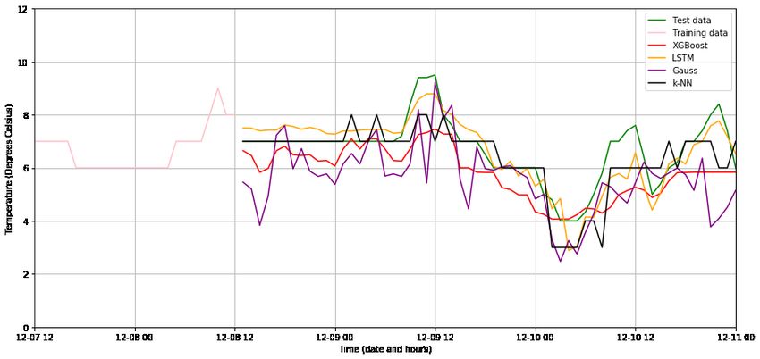
Four different machine learning methods; k-NN, XGBoost, GPR and LSTM are plotted together in Figure
19. The pink graph in Figure 19 is the training data, the black is k-NN and the purple is the GPR method.
The green graph shows the true value of the temperature inside the greenhouse, the yellow is the LSTM
method and the red is the XGBoost method.
Figure 19: The different machine learning methods plotted together with time on the X-axis in the unit of
dates and hours. The Y-axis is the temperature in degrees Celsius (◦ C). The pink graph is the training data,
the black is the k-NN method, the purple is the GPR method, the yellow is the LSTM method and the red
is the XGBoost method. The true value is the green graph.
20Figure 20 shows the data together with the two different machine learning methods LSTM and XGBoost.
Figure 20: The methods LSTM and XGBoost plotted with time on the X-axis. The Y-axis is the temperature
in degrees Celsius (◦ C). The pink graph shows the training data, the yellow is the LSTM method and the
red is the XGBoost method. The real value is the green graph.
The XGBoost method for humidity is shown in Figure 21.
Figure 21: The method XGBoost predicting the humidity in October 2018. The orange line is the training
data, the green line is the XGBoost model and the blue line is the real values from Bitroots sensor. The
y-axis is the humidity in percent and the x-axis is the time in dates and hours.
3.3 Application
The application became a website on a local network and it was designed with two figures, Figure 22 and
23. The temperature in the greenhouse is illustrated in Figure 22 and the red warning dots was set to warn
when the temperature goes under 15◦ C. The application predicts the temperature in the greenhouse for the
next two days.
21Figure 22: The temperature figure available in the application. The black line is the true temperature in
the greenhouse according to Bitroot’s sensors and the green line is the prediction. The light green area is
the confidence interval and the red dots displays the warnings of when the temperature will go too low. The
temperature is located on the y-axis and is in the unit degrees Celsius (◦ C). The time, in date and hours, is
on the x-axis.
In Figure 23 there is a plot of the predicted humidity for the next couple of days. The prediction was taken
from the application May 22, 2019.
Figure 23: The humidity figure in the application. The black line is what the humidity actually was in the
greenhouse according to Bitroots sensors and the pink line is the prediction. The x-axis is displaying the
time and the y-axis is displaying the humidity in the unit percent.
224 Discussion
4.1 Temperature
It was essential that the machine learning method could understand the circadian rhythm as well as the
seasons pattern and this is why the illumination data was created even though it was not available at the
API of SMHI.
Figure 6 shows the temperature inside and outside of the greenhouse as well as the illumination data during
two days in July, 2018. The graph shows both the illumination and the temperature outside and this illus-
trates a fair representation of the circadian rhythm that was mentioned before. Figure 6 also illustrates that
when the outside temperature increases then the temperature in the greenhouse increases. Furthermore it is
shown that the temperature inside the greenhouse (the green line) is more varying and can change quickly
even though the temperature outside (the orange line) is rather consistent. The ups and downs in the inside
temperature could depend on that the sensor perhaps was in direct sunlight and would therefore become
hotter than it normally was. This shows clearly the need for this project, predicting the temperature inside
the greenhouse simplifies for the farmer by showing the optimal way of heating the greenhouse.
Early in the project the model were tested with the following parameters; seconds of sunlight per hour,
amount of rain, wind speed, air temperature, humidity, air pressure and amount of clouds. Since the API
from SMHI did not have any data containing sunlight, the data of sunlight was replaced with data of UV-
index. While running the model it became clear that only the air temperature, the wind speed, the humidity
and the UV-index had enough importance to matter for the prediction.
The impact on the temperature inside the greenhouse from these parameters are visualised in Figure 5.
It visualises that the temperature outside the greenhouse as well as the illumination has the greatest impact
on the temperature inside the greenhouse. This agrees well to Figure 7 and 8 which both show a distinct
correlation between the temperature inside the greenhouse and the temperature outside as well as the illu-
mination. Figure 9 also illustrates a clear correlation between the temperature inside the greenhouse and the
humidity outside, even though it is not as definite as between the temperature inside and the temperature
outside as well as the illumination. This behaviour is also shown in Figure 5 where the parameter humidity
is the third most important parameter. Wind speed was another of the important parameters. Figure 10
shows the correlation between the temperature inside the greenhouse and the wind speed outside. The plot
is more scattered than the other graphs showing correlations between the temperature inside the greenhouse
and the other parameters of interest. This is also illustrated in Figure 5 where wind speed is the parameter
of least importance.
The data of the amount of clouds would probably have been a good contribution for the prediction since
clouds affects the amount of sunlight reaching the greenhouse. Figure 13 illustrates the amount of clouds
plotted against the illumination. There is no clear correlation between the two parameters. This could be
explained by that the data of the amount of clouds had an insufficient amount of data and for that reason
there were no clear correlation and it would not improve the prediction.
The other two factors, amount of rain and air pressure, were not included while making the prediction
because they were shown to be irrelevant for the outcome of the line. In Figure 11 and 12 it is visualised
that there is no true correlation between the temperature inside the greenhouse and the rain as well as the
air pressure. Figure 11 shows an unusual amount of zeros, this could depend on that it did not rain much
last year and that all of the NaN values were changed into zeroes.
234.2 Humidity
The relations between the humidity and the weather are shown in Figures 15-18. Figure 14 shows how
important every different weather type is for the machine learning model. The strongest correlation is
between the humidity inside of the greenhouse and the humidity outside the greenhouse as illustrated in
Figure 15. When the humidity inside the greenhouse varies the humidity outside behaves in a proportional
way. This is also visualised in 14 where humidity is the most important parameter. Temperature and
illumination are essential features which are shown in Figure 16 and 17. There are clear correlations between
the humidity and the outside temperature as well as the illumination even if they are not as visible as
between the humidity inside and outside the greenhouse. When the temperature outside the greenhouse or
the illumination increase the humidity inside the greenhouse decrease. Figure 14 shows how little impact
the wind speed had on the machine learning model compared to the other features of interest. This is also
shown in Figure 18 where there are no clear correlation between the humidity inside of the greenhouse and
the wind speed.
4.3 Machine learning
When choosing machine learning method it was decided that the method XGBoost (the red graph in Figure
19) should be used because it was the fastest method as well as it had the best performance when comparing
the Cross Validation score. This can be seen in table 1. The other options were the k-NN method, the
GPR method and the LSTM method which are shown in Figure 19. The GPR method performed well
but it took a long time for it to run and therefore it was not selected. The k-NN method did not have
an accurate prediction and was not selected even though it was the fastest method. The LSTM method
was the second most accurate fit for the curve but it was not selected because it works best if you have
a lot of different variables. In the end only four different variables were used which is not enough for the
LSTM method. Figure 20 shows the prediction done with both LSTM and XGBoost. Here LSTM seems
to be a better fit to the true temperature while XGBoost is most of the time located below the true val-
ues. XGBoost does not look as smooth as LSTM and struggles to follow the true peaks. XGBoost beats
LSTM according to the Cross Validation. This might be because of that the different methods function
differently depending on the season of the year which suggests that XGBoost could be better than LSTM for
other dates. Figure 20 illustrates the models operating in the winter when LSTM probably perform better
then XGBoost. XGBoost outperforms LSTM when observing a whole year according to the Cross Validation.
The XGBoost method was also chosen for the humidity. The prediction in Figure 21 shows how bad the
prediction became for the humidity. In the figure you can see that the humidity was constantly around 100%
all the time and when the data dropped towards 60%, the XGBoost model (the green line in Figure 21)
did not go down to more than 90%. This was due to that Bitroots data for the humidity was around 100%
most of the time from late September to December 2018. That was one reason to why it was difficult for
the model to predict the correct value. Another reason may be that the water content is to complex for the
parameters that have been used. For different temperatures (inside and outside) the humidity may work in
different ways. It is possible that if it was the humidity and temperature difference that where compared
then maybe there would have been other results. In this project such factors where not overlooked which
could effect why the predictions where not good.
4.4 Application
The application that was made for the farmer had two plots, one for the temperature and one for the hu-
midity. Figure 22, predicted the temperature well. The confidential interval helps the farmer understand
how much the temperature can vary. The confidential interval is bigger during the day than it is during
the night. This is good because the most critical time and the time when the farmer really needs help is
during the night. The red dots in the figure shows when the temperature is going to be under 8◦ C, but in
the Figure 22 the warning was made to appear when the temperature is going under 15◦ C. The warning
24limit was changed in this way just to illustrate how the warning dots would look like and work when they
appeared on the screen. In the real version of the application the limit was on 8◦ C since the farmer said
that the tomatoes would not like it if it was too cold. The result in Figure 22 shows is that the prediction
is good because it has the true value inside of the confidential interval. The black line faces the green line
well. The accuracy of this prediction is based on the prediction SMHI makes for the next 40 hours, so the
accuracy SMHI has on their prediction is transferred to the accuracy this prediction has.
The other figure, Figure 23 predicted the humidity. The greenhouse should not exceed 60%, which it
did according to Figure 23. The prediction in Figure 23 looks accurate but the total prediction did not
represent the humidity well, seen in Figure 21. This is probably because Bitroots humidity data from 2018
was constantly high during a long time of the Autumn part of the year and that made the prediction bad.
4.5 Improvement potential
A major issue were the lack of data points as well as missing data. If the data of amounts of clouds, amount
of rain and air pressure were more complete they could affect the result in a positive way. Thereby an
improvement would be to include them in the model. Also the parameters that was important missed a few
values. They could give an even better outcome if they were complete. The amount of data from SMHI and
its quality is hard to control or improve, but there are websites containing more preferable data that costs.
This project was made with limited resources and therefore buying data was not an option, but it could be
a good improvement of the project. It would also be good if the training data had been over a year instead
of the period of June-December 2018.
The API of SMHI does not include historical data. By using another supplier of data there might be
possible to retrieve historical data by their API. If this was possible, the method could be trained continu-
ously while it is running. Then the prediction would be improved as time goes on and the machine learning
method would be more accurate over time.
The data provided by Bitroot had some flaws. The humidity data did occasionally not show a realistic
view of the reality due to missing and misleading values, this data would probably be better in the future
when the sensors have developed and provide more accurate values. The data of the temperature was bet-
ter but sometimes it showed temperature peaks of around 200◦ C. Bitroot is a start up company and their
products are constantly being developed. As time pass, their sensors and data could improve.
A potential way to improve the illumination model would be if some data of the amount of clouds could be
linked to the sun data. For example if the amount of clouds could be translated to a factor that could affect
the illumination data. That would be a good improvement of the illumination data.
4.6 Development opportunities
One deficiency of the project is that the machine learning model is trained on data from one specific green-
house and the area nearby. It is rather easy to train a new model with other data but that needs a large
data set before the new model can start training. This implies that it is a long term project that needs to
be re-installed for every new greenhouse it is applied for. It means the model gets better gradually as the
amount of data grows. An interesting development of the project would be either testing the already learned
model at a new greenhouse or learning a new model by data from other greenhouses. This would make the
product more versatile.
25You can also read