Program MARK: Survival Estimation from Populations of Marked Animals
←
→
Page content transcription
If your browser does not render page correctly, please read the page content below
Program MARK: Survival Estimation from Populations of Marked Animals

GARY C. WHITE1 and KENNETH P. BURNHAM2 1Department of Fishery and Wildlife
Biology, Colorado State University, Fort Collins, CO 80523, USA and 2Colorado Cooperative
Fish and Wildlife Research Unit, Colorado State University, Fort Collins, CO 80523, USA.

SUMMARY
        Program MARK, a Windows 95 program, provides parameter estimates from marked
animals when they are re-encountered at a later time. Re-encounters can be from dead
recoveries (e.g., the animal is harvested), live recaptures (e.g. the animal is re-trapped or re-
sighted), radio tracking, or from some combination of these sources of re-encounters. The time
intervals between re-encounters do not have to be equal, but are assumed to be 1 time unit if not
specified. More than one attribute group of animals can be modeled, e.g., treatment and control
animals, and covariates specific to the group or the individual animal can be used. The basic
input to program MARK is the encounter history for each animal. MARK can also provide
estimates of population size for closed populations. Capture (p) and re-capture (c) probabilities
for closed models can be modeled by attribute groups, and as a function of time, but not as a
function of individual-specific covariates.
        Parameters can be constrained to be the same across re-encounter occasions, or by age,
or by group, using the parameter index matrix (PIM). A set of common models for screening
data initially are provided, with time effects, group effects, time × group effects, and a null model
of none of the above provided for each parameter. Besides the logit function to link the design
matrix to the parameters of the model, other link functions include the log-log, complimentary
log-log, sine, log, and identity.
        Program MARK computes the estimates of model parameters via numerical maximum
likelihood techniques. The FORTRAN program that does this computation also determines
numerically the number of parameters that are estimable in the model, and reports its guess of
one parameter that is not estimable if one or more parameters are not estimable. The number of
estimable parameters is used to compute the quasi-likelihood AIC value (QAICc) for the model.
        Outputs for various models that the user has built (fit) are stored in a database, known as
the Results Database. The input data are also stored in this database, making it a complete
description of the model building process. The database is viewed and manipulated in a Results
Browser window.
        Summaries available from the Results Browser window include viewing and printing
model output (estimates, standard errors, and goodness-of-fit tests), deviance residuals from the
model (including graphics and point and click capability to view the encounter history
responsible for a particular residual), likelihood ratio and analysis of deviance (ANODEV)
between models, and adjustments for over dispersion. Models can also be retrieved and
modified to create additional models.
        These capabilities are implemented in a Microsoft Windows 95 interface. Context-
sensitive help screens are available with Help click buttons and the F1 key. The Shift-F1 key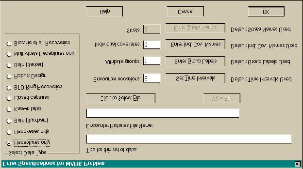
Program MARK: Survival Estimation from Populations of Marked Animals                              2

can also be used to investigate the function of a particular control or menu item. Help screens
include hypertext links to other help screens, with the intent to provide all the necessary
program documentation on-line with the Help System.
Program MARK: Survival Estimation from Populations of Marked Animals                                       3

INTRODUCTION
         Expanding human populations and extensive habitat destruction and alteration continue to
impact the world's fauna and flora. As a result, monitoring of biological populations has begun to
receive increasing emphasis in most countries, including the less developed areas of the world.1 Use of
marked individuals and capture-recapture theory play an important role in this process. Further, risk
assessment 2,3 in higher vertebrates can be done in the framework of capture-recapture theory.
Population viability analyses must rely on estimates of vital rates of a population; often these can only be
derived from the study of uniquely marked animals. The richness component of biodiversity can often
be estimated in the context of closed model capture-recapture.4, 5 Finally, the monitoring components
of adaptive management6 can be rigorously addressed in terms of the analysis of data from marked
subpopulations.
         Capture-recapture surveys have been used as a general sampling and analysis method to assess
population status and trends in many biological populations.7 The use of marked individuals is
analogous to the use of various tracers in studies of physiology, medicine and nutrient cycling. Recent
advances in technology allow a wide variety of marking methods.8
         The motivation for developing Program MARK was to bring a common programming
environment to the estimation of survival from marked animals. Marked animals can be re-encountered
as either live or dead, in a variety of experimental frameworks. Prior to MARK, no program easily
combined the estimation of survival from both live and dead re-encounters, nor allowed for the
modeling of capture and re-capture probabilities in a general modeling framework for estimation of
population size in closed populations.
         The purpose of this paper is to describe the general features of Program MARK, and provide
users with a general idea of how the program operates. Documentation for the program is provided in
the Help File that is distributed with the program. Specific details for all the menu options and dialog
controls are provided in the Help File.
         We assume the reader knows the basics about the Cormack-Jolly-Seber,9-13 capture-
recapture,14-18 and recovery models,19-22 including concepts like the logit-link to incorporate covariates
into models with a design matrix,23-24 multi-group models, model selection25 with AIC,26 and maximum
likelihood parameter estimation.13 Cooch et al. 27 explain many of these basics in a general primer,
although the material is focused on the SURGE program. In addition, the user must have some
familiarity with the Windows 95 operating system. The objective of this paper is to describe how these
methods can be used in Program MARK.
TYPES OF ENCOUNTER DATA USED BY PROGRAM MARK
         Program Mark provides parameter estimates for 5 types of re-encounter data: (1) Cormack-
Jolly- Seber models (live animal recaptures that are released alive), (2) band or ring recovery models
(dead animal recoveries), (3) models with both live and dead re-encounters, (4) known fate (e.g.,
radio-tracking) models, and (5) some closed capture-recapture models.
Live Recaptures
         Live recaptures are the basis of the standard Cormack-Jolly-Seber (CJS) model. Marked
animals are released into the population, usually by trapping them from the population. Then, marked
animals are encountered by catching them alive and re-releasing them, or often just a visual resighting.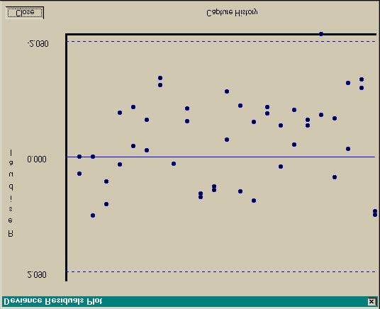
Program MARK: Survival Estimation from Populations of Marked Animals                                         4

If marked animals are released into the population on occasion 1, then each succeeding capture
occasion is one encounter occasion. Consider the following scenario:

                                                                       Encounter History

                                                     Seen                    11 φ p
                                         p
                             Live
                  φ
Releases                         1− p                Not Seen                10 φ( 1 − p )
            1− φ             Dead or
                                                                             10 1 − φ
                             Emigrated
Animals survive from initial release to the second encounter with probability S1 , from the second
encounter occasion to the third encounter occasion with probability S2 , etc. The recapture probability
at encounter occasion 2 is p2 , p3 is the recapture probability at encounter occasion 3, etc. At least 2
re-encounter occasions are required to estimate the survival probability ( S1 ) between the first release
occasion and the next encounter occasion in the full time-effects model. The survival probability
between the last two encounter occasions is not estimable in the full time-effects model because only
the product of survival and recapture probability for this occasion is identifiable.
         Generally, as in the diagram, the conditional survival probabilities of the CJS model are labeled
as 1, φ2 , etc., because the quantity estimated is the probability of remaining available for recapture.
Thus, animals that emigrate from the study area are not available for recapture, so appear to have died
in this model. Thus, φi = Si (1 − Ei ) , where Ei is the probability of emigrating from the study area,
and φi is termed 'apparent' survival, as this parameter is technically not the survival probability of
marked animals in the population. Rather, φi is the probability that the animal remains alive and is
available for recapture.
        Estimates of population size ( N̂ ) or births and immigration ( B̂) of the Jolly-Seber model are not
provided in Program MARK, as in POPAN-428-29 or JOLLY and JOLLYAGE. 12
Dead Recoveries
        With dead recoveries (i.e., band, fish tag, or ring recovery models), animals are captured from
the population, marked, and released back into the population at each occasion. Later, marked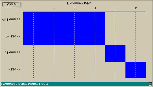
Program MARK: Survival Estimation from Populations of Marked Animals                                       5

animals are encountered as dead animals, typically from harvest or just found dead (e.g., gulls). The
following diagram illustrates this scenario:
                                                                 Encounter History

                            Live                                       10 S
                  S
 Releases                                        Reported              11 (1 - S)r
                                        r
            1-S             Dead
                                  1-r
                                                 Not                   10 (1 - S)(1 - r)
                                                 Reported
Marked animals are assumed to survive from one release to the next with survival probability Si . If
they die, the dead marked animals are reported during each period between releases with probability
 ri . The survival probability and reporting probability prior to the last release can not be estimated
individually in the full time-effects model, but only as a product. This parameterization differs from that
of Brownie et al.21 in that their f i is replaced as f i = (1 − S i )ri . The ri are equivalent to the λi of
life table models.30-31 The reason for making this change is so that the encounter process, modeled with
the ri parameters, can be separated from the survival process, modeled with the Si parameters. With
the f i parameterization, the 2 processes are both part of this parameter. Hence, developing more
advanced models with the design matrix options of MARK is difficult, if not illogical with the f i
parameterization. However, the negative side of this new parameterization is that the last Si and ri are
confounded in the full time-effects model, as only the product (1 − S i ) ri is identifiable, and hence
estimable.
Both Live and Dead Encounters
        The model for the joint live and dead encounter data type was first published by Burnham,32 but
with a slightly different parameterization than used in Program MARK. In MARK, the dead
encounters are not modeled with the f i of Burnham32, but rather as f i = (1 − Si )ri , as discussed
above for the dead encounter models. The method is a combination of the 2 above, but allows the
estimation of fidelity ( Fi = 1 − E i ), or the probability that the animal remains on the study area and is
available for capture. As a result, the estimates of Si are estimates of the survival probability of the
marked animals, and not the apparent survival ( φi = Si Fi ) as discussed for the live encounter model.
Program MARK: Survival Estimation from Populations of Marked Animals 6
In the models discussed so far, live captures and resightings modeled with the pi parameters
are assumed to occur over a short time interval, whereas dead recoveries modeled with the ri
parameters extend over the time interval. The actual time of the dead recovery is not used in the
estimation of survival for 2 reasons. First, it is often not known. Second, even if the exact time of
recovery is known, little information is contributed if the recovery probability ( ri ) is varying during the
time interval.
Known Fates
Known fate data assumes that there are no nuisance parameters involved with animal captures
or resightings. The data derive from radio-tracking studies, although some radio-tracking studies fail to
follow all the marked animals and so would not meet the assumptions of this model (they then would
need to be analyzed by mark-encounter models). A diagram illustrating this scenario is
S1 S2 S3
Release Encounter 2 Encounter 3 Encounter 4 ...
where the probability of encounter on each occasion is 1 if the animal is alive.
Closed Captures
Closed-capture data assume that all survival probabilities are 1.0 across the short time intervals
of the study. Thus, survival is not estimated. Rather, the probability of first capture ( pi ) and the
probability of recapture ( ci ) are estimated, along with the number of animals in the population ( Ni ).
The diagram describing this scenario looks like the following:
Occasion 1 Occasion 2 Occasion 3 Occasion 4 ...
p1 p2 p3 p4 First Encounter
c2 c3 c4 Additional Encounter(s)
where the ci recapture probability parameters are shown under the initial capture ( pi ) parameters.
This data type is the same as is analyzed with Program CAPTURE.15 All the likelihood models in
CAPTURE can be duplicated in MARK. However, MARK allows additional likelihood-based
models not available in CAPTURE, plus comparisons between groups and the incorporation of time-
specific and/or group-specific covariates into the model.
The main limitation of MARK for closed capture-recapture models is the lack of models
incorporating individual heterogeneity. Individual covariates cannot be used in MARK with this data
type because existing models in the literature33-34 have not yet been implemented.
Other Models
Models for other types of encounter data are also available in Program MARK, including the
robust design model,35-37 multi-strata model,38-39 Barker’s40 extension to the joint live and dead
encounters model, ring recovery models where the number of birds marked is unknown, and the
Brownie et al.21 parameterization of ring recovery models.
PROGRAM OPERATION
Program MARK is operated by a Windows 95 interface. A "batch " file mode of operation is
available in that the numerical procedure reads an ASCII input file. However, models are constructed
interactively with the interface much easier than creating them manually in an ASCII input file.
Interactive and context-sensitive help is available at any time while working in the interface program.
The Help System is constructed with the Windows Help System, so is likely familiar to most users. NoProgram MARK: Survival Estimation from Populations of Marked Animals 7
printed documentation on MARK (other than this manuscript) is provided; all documentation is
contained in the Help System, thus insuring that the documentation is current with the current version of
the program.
All analyses in MARK are based on encounter histories. To begin construction of a set of
models for a data set, the data must first be read by MARK from the Encounter Histories file. Next,
the Parameter Index Matrices (PIM) can be manipulated, followed by the Design Matrix. These tools
provide the model specifications to construct a broad array of models. Once the model is fully
specified, the Run Window is opened, where the link function is specified and currently must be the
same for all parameters, parameters can be "fixed " to specific values, and the name of the model is
specified. Once a set of models has been constructed, likelihood ratio tests between models can be
computed, or Analysis of Deviance (ANODEV) tables constructed.
To begin an analysis, you must create an Encounter Histories file using an ASCII text editor,
such as the NotePad or WordPad editors that are provided within Windows 95. The format of the
Encounter Histories file is similar in general to that of Program RELEASE,41 and is identical to Program
RELEASE form for live recapture data without covariates. MARK does not provide data management
capabilities for the encounter histories. Once the Encounter Histories file is created, start Program
MARK and select File, New. The dialog box shown in Fig. 1 appears.
As shown in the middle of Fig. 1, you are requested to enter the number of encounter
occasions, number of groups (e.g., sex, ages, areas), number of individual covariates, and only if the
multi-strata model was selected, the number of strata. Each of these variables can have additional
input, accomplished by clicking the push button next to the input box. On the left side, you specify the
type of data. Just to the right, you specify the title for the data, and the name of the Encounter Histories
file, with a push button to help you find the file, plus a second push button the examine the contents of
the file once you have selected it. At the bottom of the screen is the OK button to proceed once you
have entered the necessary information, a Cancel button to quit, and a Help button to obtain help from
the help file. You can also hit the Shift-F1 key when any of the controls on the window are highlighted
to obtain context-sensitive help for that specific control.
Encounter Histories File
To provide the data for parameter estimation, the Encounter Histories file is used. This file
contains the encounter histories, i.e., the raw data needed by Program MARK. Format of the file
depends on the data type, although all data types allow a conceptually similar encounter history format.
The convention of Program Mark is that this file name ends in the INP suffix. The root part of an
Encounter Histories file name dictates the name of the dBASE file used to hold model results. For
example, the input file MULEDEER.INP would produce a Results file with the name
MULEDEER.DBF and 2 additional files (MULEDEER.FPT and MULEDEER.CDX) that would
contain the memo fields holding model output and index ordering, respectively. Once the DBF, FPT,
and CDX files are created, the INP file is no longer needed. Its contents are now part of the DBF file.
Encounter Histories files do not contain any PROC statements (as in Program RELEASE), but
only encounter histories or recovery matrices. You can have group label statements and comment
statements in the input file, just to help you remember what the file contains. Remember to end theseProgram MARK: Survival Estimation from Populations of Marked Animals 8
statements with a semicolon. The interactive interface adds the necessary program statements to
produce parameter estimates with the numerical algorithm based on the model specified.
The Encounter Histories file is incorporated into the results database created to hold parameter
estimates and other results. Because all results in the results database depend on the encounter
histories not changing, you cannot change the input. Even if you change the values in the Encounter
Histories file, the Results file will not change. The only way to produce models from a changed
Encounter Histories file is to incorporate the changed file into a new results database (hence, start
over). You can view the encounter histories in the results database by having it listed in the results for a
model by checking the list data checkbox in the Run Window.
Some simplified examples of Encounter Histories files follow. The full set of data for each
example is provided in the Program MARK help file, and as an example input file distributed with the
program.
First is a live recapture data set with 2 groups and 6 encounter occasions. Note that the release
occasion is counted as an encounter occasion (in contrast to the protocol used in Program SURGE).
The encounter history is coded for just the live encounters, i.e.,
LLLLLL
and the initial capture is counted as an encounter occasion. Again, the encounter histories are given,
with 1 indicating a live capture or recapture, and 0 meaning not captured. The number of animals in
each group follows the encounter history. Negative values indicate animals that were not released again,
i.e., losses on capture. The following example is the partial input for the example data in Burnham et
al.41 (page 29). As you might expect, any input file used with Program RELEASE will work with
MARK if the RELEASE-specific PROC statements are removed.
100000 25925 24605;
100001 563 605;
100001 -27 -36;
...
110100 67 68;
110100 -3 -4;
110101 1 2;
110110 2 1;
111000 10 12;
111001 0 1;
111100 1 0;
Next, a joint live recapture and dead recovery encounter histories file is shown, with only one
group, but 5 encounter occasions. The encounter histories are alternating live (L) recaptures and dead
(D) recoveries, i.e.,
LDLDLDLDLD
with 1 indicating a recapture or recovery, and 0 indicating no encounter. Encounter histories always
start with an L and end with a D in Program MARK (this is not restrictive if the actual data end with a
live capture). The number after the encounter history is the number of animals with this history for
group 1, just as with Program RELEASE. Following the frequency for the last group, a semi-colon is
used to end the statement. Note that a common mistake is to not end statements with semicolons.Program MARK: Survival Estimation from Populations of Marked Animals 9
1000000000 41152;
1000000001 1923;
1000000010 557;
1000000011 103;
1000000100 2897;
...
1010101010 184;
1010101011 24;
1010101100 144;
1010110000 583;
1011000000 2672;
1100000000 15153;
The next example is the summarized input for a dead recovery data set with 15 release
occasions and 15 years of recovery data. Even though the raw data are read as recovery matrices,
encounter histories are created internally in MARK. The triangular matrices represent 2 groups;
adults, followed by young. Following each upper-triangular matrix is the number of animals marked
and released into the population each year. This format is similar to that used by Brownie et al.21 The
input lines identified with the phrase "recovery matrix" are required to identify the input as a recovery
matrix, and are not interpreted as an encounter history.
recovery matrix group=1;
7 4 1 0 1 0 0 0 0 0 0 0 0 0 0;
8 5 1 0 0 0 0 0 0 0 0 0 0 0;
10 4 2 0 1 1 0 0 0 0 0 0 0;
16 3 2 0 0 0 0 0 0 0 0 0;
12 3 2 3 0 0 0 0 0 0 0;
10 9 3 0 0 0 0 0 0 0;
14 9 3 3 0 0 0 0 0;
9 5 2 1 0 1 0 0;
16 5 2 0 1 0 0;
19 6 2 1 0 1;
15 3 0 0 0;
8 5 1 0;
10 1 0;
8 1;
10;
99 88 153 114 123 98 146 173 190 190 157 92 88 51 85;
recovery matrix group=2;
6 4 6 1 0 1 0 0 0 0 0 0 0 0 0;
6 5 2 1 0 0 0 0 0 0 0 0 0 0;
18 6 6 2 0 1 0 0 0 0 0 0 0;
17 5 6 2 1 1 0 0 0 0 0 0;
20 9 6 2 1 1 0 0 0 0 0;
14 4 3 1 0 0 0 0 0 0;
13 4 0 1 0 0 0 0 0;
13 5 3 1 0 0 0 0;
13 5 4 0 0 0 0;
7 1 3 1 1 0;
15 10 2 0 0;
12 4 0 0;
16 4 1;
5 2;
8;
80 54 138 120 183 106 111 127 110 110 152 102 163 104 117;Program MARK: Survival Estimation from Populations of Marked Animals 10
No automatic capability to handle non-triangular recovery matrices has been included in MARK. Non-
triangular matrices are generated when marking new animals ceases, but recoveries are continued.
Such data sets can be handled by forming a triangular recovery matrix with the additions of zeros for
the number banded and recovered. During analysis, the parameters associated with these zero data
should be fixed to logical values (i.e., ri = 0) to reduce numerical problems with non-estimable
parameters.
Dead recoveries can also be coded as encounter histories in the
LDLDLDLDLDLD
format. The following is an example of only dead recoveries, because a live animal is never captured
alive after its initial capture. That is, none of the encounter histories have more than a single 1 in an L
column. This example has 15 encounter occasions and 1 group.
000000000000000000000000000010 465;
000000000000000000000000000011 35;
000000000000000000000000001000 418;
000000000000000000000000001001 15;
000000000000000000000000001100 67;
...
100000010000000000000000000000 11;
100001000000000000000000000000 9;
100100000000000000000000000000 51;
110000000000000000000000000000 33;
The next example is the input for a data set with known fates. As with dead recovery matrices,
the summarized input is used to create encounter histories. Each line presents the number of animals
monitored for one time interval, in this case, a week. The first value is the number of animals
monitored, followed by the number that died during the interval. Each group is provided in a separate
matrix. In the following example, a group of black ducks are monitored for 8 weeks.42 Initially, 48
ducks were monitored, and 1 died during the first week. The remaining 47 ducks were monitored
during the second week, when 2 died. However, 4 more were lost from the study for other reasons,
i.e., resulting in a reduction in the numbers of animals monitored. As a result, only 41 ducks were
available for monitoring during the third week. The phrase "known fate" on the first line of input is
required to identify the input as this special format, instead of the usual encounter history format.
known fate group=1;
48 1;
47 2;
41 2;
39 5;
32 4;
28 3;
25 1;
24 0;
The following input is an example of a closed capture-recapture data set. The capture histories
are specified as a single 1 or 0 for each occasion, representing captured (1) or not captured (0).
Following the capture history is the frequency, or count of the number of animals with this capture
history, for each group. In the example, 2 groups are provided. Individual covariates are not allowedProgram MARK: Survival Estimation from Populations of Marked Animals 11
with closed captures, because the models of Huggins 33-34 have not been implemented in MARK. This
data set could have been stored more compactly by not representing each animal on a separate line of
input. The advantage of entering the data as shown with only a 0 or 1 as the capture frequency is that
the input file can also be used with Program CAPTURE.
0101010 1 0;
0011000 1 0;
1001100 1 0;
1100101 1 0;
...
1000101 0 1;
0100000 0 1;
1010100 0 1;
1001010 0 1;
Additional examples of encounter history files are provided in the help document distributed with
the program.
Parameter Index Matrices
The Parameter Index Matrices (PIM), allow constraints to be placed on the parameter estimates.
There is a parameter matrix for each type of basic parameter in each group model, with each parameter
matrix shown in its own window. As an example suppose that 2 groups of animals are marked. Then,
for live recaptures, 2 Apparent Survival ( φ ) matrices (Windows) would be displayed, and 2
Recapture Probability (p) matrices (Windows) would be shown. Likewise, for dead recovery data for
2 groups, 2 Survival (S) matrices and 2 reporting probability (r) matrices would be used, for 4
windows. When both live and dead recoveries are modeled, each group would have 4 parameters
types: S, r, p, and F. Thus, 8 windows would be available. Only the first window is opened by default.
Any (or all) of the PIM windows can be opened from the PIM menu option. Likewise, any PIM
window that is currently open can be closed, and later opened again.
The parameter index matrices determine the number of basic parameters that will be estimated
(i.e., the number of rows in the design matrix), and hence, the PIM must be constructed before use of
the Design Matrix window. PIMs may reduce the number of basic parameters, with further constraints
provided by the design matrix. Commands are available to set all the parameter matrices to a particular
format (e.g., all constant, all time-specific, or all age-specific), or to set the current window to a
particular format.
Included on the PIM window are push buttons to Close the window (but the values of parameter
settings are not lost; they just are not displayed), Help to display this help screen, PIM Chart to
graphically display the relationship among the PIM values, and + and - to increment or decrement,
respectively, all the index values in the PIM Window by 1.
Parameter matrices can be manipulated to specify various models. The following are the
parameter matrices for live recapture data to specify a { φ (g*t) p(g*t)} model for a data set with 5
encounter occasions (resulting in 4 survival intervals and 4 recapture occasions) and 2 groups.Program MARK: Survival Estimation from Populations of Marked Animals 12
Apparent Survival Group 1
1 2 3 4
2 3 4
3 4
4
Apparent Survival Group 2
5 6 7 8
6 7 8
7 8
8
Recapture Probabilities Group 1
9 10 11 12
10 11 12
11 12
12
Recapture Probabilities Group 2
13 14 15 16
14 15 16
15 16
16
In this example, parameter 1 is apparent survival for the first interval for group 1, and parameter 2 is
apparent survival for the second interval for group 1. Parameter 7 is apparent survival for the third
interval for group 2, and parameter 8 is apparent survival for the fourth interval for group 2. Parameter
9 is the recapture probability for the second occasion for group 1, parameter 10 is the recapture
probability for the third occasion for group 1. Parameter 15 is the recapture probability for the fourth
occasion for group 2, and parameter 16 is the recapture probability for the fifth occasion for group 2.
Note that the capture probability for the first occasion does not appear in the Cormack-Jolly-Seber
model, and thus does not appear in the parameter index matrices for recapture probabilities.
To reduce this model to { φ (t) p(t)}, the following parameter matrices would work.Program MARK: Survival Estimation from Populations of Marked Animals 13
Apparent Survival Group 1
1 2 3 4
2 3 4
3 4
4
Apparent Survival Group 2
1 2 3 4
2 3 4
3 4
4
Recapture Probabilities Group 1
5 6 7 8
6 7 8
7 8
8
Recapture Probabilities Group 2
5 6 7 8
6 7 8
7 8
8
In the above example, the parameters by time and type are constrained equal across groups.
The following parameter matrices have no time effect, but do have a group effect. Thus, the
model is {φ (g) p(g)}.
Apparent Survival Group 1
1 1 1 1
1 1 1
1 1
1
Apparent Survival Group 2
2 2 2 2
2 2 2
2 2
2
Recapture Probabilities Group 1
3 3 3 3
3 3 3
3 3
3
Recapture Probabilities Group 2
4 4 4 4
4 4 4
4 4
4
Additional examples of PIMs demonstrating age and cohort models are provided with the Help system
that accompanies the program. Also Cooch et al. 27 provide many more examples of how to structure
the parameter indices.Program MARK: Survival Estimation from Populations of Marked Animals 14
The Parameter Index Chart displays graphically the relationship of parameters across the attribute
groups and time (Fig. 2). The concept of a PIM derives from program SURGE, 13, 43 with graphical
manipulation of the PIM first demonstrated by Program SURPH.44 However, a key difference in the
implementation in MARK from SURGE is that the PIMs can allow overlap of parameter indices across
parameters types, and thus the same parameter estimate could be used for both a φ and a p. Although
such a model is unlikely for just live recaptures or dead recoveries, we can visualize such models with
joint live and dead encounters.
Design Matrix
Additional constraints can be placed on parameters with the Design Matrix. The concept of a
design matrix comes from general linear models (GLM).23 The design matrix ( X ) is multiplied by the
parameter vector ( ) to produce the original parameters ( φ , S , p, r , etc.) via a link function. For
instance,
logit(θ ) = X β
uses the logit link function to link the design matrix to the vector of original parameters (θ ). The
elements of θ are the original parameters, whereas the columns of matrix X correspond to the
reduced parameter vector β . The vector β can be thought of as the “likelihood parameters” because
they appear in the likelihood. They are linked to the derived, or real parameters, θ .
Assume that the PIM model is { φ (g*t) p(g*t)} as shown in the text above for 5 encounter
occasions. To specify the fully additive {φ (g+t) p(g+t)} model where parameters vary temporally in
parallel, the design matrix must be used. The design matrix is opened with the Design menu option.
The design matrix always has the same number of rows as there are parameters in the PIMs.
However, the number of columns can be variable. A choice of Full or Reduced is offered when the
Design menu option is selected. The Full Design Matrix has the same number of columns as rows and
defaults to an identity matrix, whereas the Reduced Design Matrix allows you to specify the number of
columns and is initialized to all zeros. Each parameter specified in the PIMs will now be computed as a
linear combination of the columns of the design matrix. Each parameter in the PIMs has its own row in
the design matrix. Thus, the design matrix provides a set of constraints on the parameters in the PIMs
by reducing the number of parameters (number of rows) from the number of unique values in the PIMs
to the number of columns in the design matrix.
The concept of a design matrix for use with capture-recapture data was taken from Program
SURGE.43 However, in MARK a single design matrix applies to all parameters, unlike SURGE where
design matrices are specific to a parameter type, i.e., either apparent survival or recapture probability.
The more general implementation in MARK allows parameters of different types to be modeled by the
same function of 1 or more covariates. As an example, parallelism could be enforced between live
recapture and dead recovery probabilities, or between survival and fidelity. Also, unlike SURGE,
MARK does not assume an intercept in the design matrix. If no design matrix is specified, the default is
an identity matrix, where each parameter in the PIMs corresponds to a column in the design matrix.
MARK always constructs and uses a design matrix.Program MARK: Survival Estimation from Populations of Marked Animals 15
The following is an example of a design matrix for the additive {φ (g+t) p(g+t)} model used to
demonstrate various PIMs with 5 encounter occasions. In this model, the time effect is the same for
each group, with the group effect additive to this time effect. In the following matrix, column 1 is the
group effect for apparent survival, columns 2-5 are the time effects for apparent survival, column 6 is
the group effect for recapture probabilities, and columns 7-10 are the time effects for the recapture
probabilities. The first 4 rows correspond to the φ for group 1, the next 4 rows for φ for group 2,
the next 4 rows for pi for group 1, and the last 4 rows for pi for group 2. Note that the coding for the
group effect dummy variable is zero for the first group, and 1 for the second group.
0 1 0 0 0 0 0 0 0 0
0 0 1 0 0 0 0 0 0 0
0 0 0 1 0 0 0 0 0 0
0 0 0 0 1 0 0 0 0 0
1 1 0 0 0 0 0 0 0 0
1 0 1 0 0 0 0 0 0 0
1 0 0 1 0 0 0 0 0 0
1 0 0 0 1 0 0 0 0 0
0 0 0 0 0 0 1 0 0 0
0 0 0 0 0 0 0 1 0 0
0 0 0 0 0 0 0 0 1 0
0 0 0 0 0 0 0 0 0 1
0 0 0 0 0 1 1 0 0 0
0 0 0 0 0 1 0 1 0 0
0 0 0 0 0 1 0 0 1 0
0 0 0 0 0 1 0 0 0 1
The Design Matrix can also be used to provide additional information from time-varying
covariates. As an example, suppose the rainfall for the 4 survival intervals in the above example is 2,
10, 4, and 3 cm. This information could be used to model survival effects with the following model,
where each group has a different intercept for survival, but a common slope. The model name would
be { φ (g+rainfall) p(g+t)}. Column 1 codes the intercept, column 2 codes the offset of the intercept
for group 2, and column 3 codes the rainfall variable.
1 0 2 0 0 0 0 0
1 0 10 0 0 0 0 0
1 0 4 0 0 0 0 0
1 0 3 0 0 0 0 0
1 1 2 0 0 0 0 0
1 1 10 0 0 0 0 0
1 1 4 0 0 0 0 0
1 1 3 0 0 0 0 0
0 0 0 0 1 0 0 0
0 0 0 0 0 1 0 0
0 0 0 0 0 0 1 0
0 0 0 0 0 0 0 1
0 0 0 1 1 0 0 0
0 0 0 1 0 1 0 0
0 0 0 1 0 0 1 0
0 0 0 1 0 0 0 1Program MARK: Survival Estimation from Populations of Marked Animals 16
A similar Design Matrix could be used to evaluate differences in the trend of survival for the 2
groups. The rainfall covariate in column 3 has been replaced by a time trend variable, resulting in a
covariance analysis on the φ 's: parallel regressions with different intercepts.
1 0 1 0 0 0 0 0
1 0 2 0 0 0 0 0
1 0 3 0 0 0 0 0
1 0 4 0 0 0 0 0
1 1 1 0 0 0 0 0
1 1 2 0 0 0 0 0
1 1 3 0 0 0 0 0
1 1 4 0 0 0 0 0
0 0 0 0 1 0 0 0
0 0 0 0 0 1 0 0
0 0 0 0 0 0 1 0
0 0 0 0 0 0 0 1
0 0 0 1 1 0 0 0
0 0 0 1 0 1 0 0
0 0 0 1 0 0 1 0
0 0 0 1 0 0 0 1
Individual covariates are also incorporated into an analysis via the design matrix. By specifying
the name of an individual covariate in a cell of the Design Matrix, you tell MARK to use the value of
this covariate in the design matrix when the capture history for each individual is used in the likelihood.
As an example, suppose that 2 individual covariates are included: age (0=subadult, 1=adult), and
weight at time of initial capture. The variable names given to these variables are, naturally, AGE and
WEIGHT. These names were assigned in the dialog box where the encounter histories file was
specified (Fig. 1). The following design matrix would use weight as a covariate, with an intercept term
and a group effect. The model name would be { φ (g+weight) p(g+t)}.
1 0 weight 0 0 0 0 0
1 0 weight 0 0 0 0 0
1 0 weight 0 0 0 0 0
1 0 weight 0 0 0 0 0
1 1 weight 0 0 0 0 0
1 1 weight 0 0 0 0 0
1 1 weight 0 0 0 0 0
1 1 weight 0 0 0 0 0
0 0 0 0 1 0 0 0
0 0 0 0 0 1 0 0
0 0 0 0 0 0 1 0
0 0 0 0 0 0 0 1
0 0 0 1 1 0 0 0
0 0 0 1 0 1 0 0
0 0 0 1 0 0 1 0
0 0 0 1 0 0 0 1
Each of the 8 apparent survival probabilities would be modeled with the same slope parameter for
WEIGHT, but on an individual animal basis. Thus, time is not included in the relationship. However, a
group effect is included in survival, so that each group would have a different intercept. Suppose you
believe that the relationship between survival and weight changes with each time interval. The followingProgram MARK: Survival Estimation from Populations of Marked Animals 17
design matrix would allow 4 different weight models, one for each survival occasion. The model would
be named { φ (g+t*weight) p(g+t)}.
1 0 weight 0 0 0 0 0 0 0 0
1 0 0 weight 0 0 0 0 0 0 0
1 0 0 0 weight 0 0 0 0 0 0
1 0 0 0 0 weight 0 0 0 0 0
1 1 weight 0 0 0 0 0 0 0 0
1 1 0 weight 0 0 0 0 0 0 0
1 1 0 0 weight 0 0 0 0 0 0
1 1 0 0 0 weight 0 0 0 0 0
0 0 0 0 0 0 0 1 0 0 0
0 0 0 0 0 0 0 0 1 0 0
0 0 0 0 0 0 0 0 0 1 0
0 0 0 0 0 0 0 0 0 0 1
0 0 0 0 0 0 1 1 0 0 0
0 0 0 0 0 0 1 0 1 0 0
0 0 0 0 0 0 1 0 0 1 0
0 0 0 0 0 0 1 0 0 0 1
Many more examples of how to construct the design matrix are provided in the Program MARK
interactive Help System. Numerous menu options are described in the Help System to avoid having to
build a design matrix manually, e.g., to fill 1 or more columns with various designs.
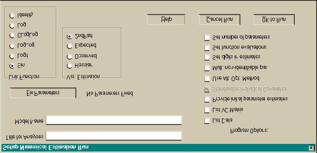
Run Window
The Run Window is opened by selecting the Run menu option. This window (Fig. 3) allows you
to specify the Run Title, Model Name, parameters to Fix to a specified value, the Link Function to be
used, and the Variance Estimation algorithm to be used. You can also select various program options
such as whether to list the raw data (encounter histories) and/or variance-covariance matrices in the
output, plus other program options that concern the numerical optimization of the likelihood function to
obtain parameter estimates.
The Title entry box allows you to modify the title printed on output for a set of data. Normally,
you will set this for the first model for which you estimate parameters, and then not change it. The
Model Name entry box is where a name for the model you have specified with the PIMs and Design
Matrix is specified. Various model naming conventions have developed in the literature, but we prefer
something patterned after the procedure of Lebreton et al.,13 as demonstrated elsewhere in the paper.
The main idea is to provide enough detail in the model name entry so that you can easily determine the
model's structure and what parameters were estimated based on the model name.
Fixing Parameters. By selecting the Fix Parameters Button on the Run Window screen, you
can select parameters to "fix", hence cause them to not be estimated. A dialog window listing all the
parameters is presented, with edit boxes to enter the value that you want the parameter to be fixed at.
By fixing a parameter, you are saying that you do not want this parameter to be estimated from the
data, but rather set to the specified value. Fixing a parameter is a useful method to determine if it is
confounded with another parameter. For example, the last φ and p are confounded in the
time-specific Cormack-Jolly-Seber model, as are the last S and r in the time-specific dead recoveries
model. You can set the last p or r to 1.0 to force the survival parameter to be estimated as the
product.Program MARK: Survival Estimation from Populations of Marked Animals 18
Link Functions. A link function links the linear model specified in the design matrix with the
survival, recapture, reporting, and fidelity parameters specified in the PIMs. Program Mark supports 6
different link functions. The default is the sin function because it is generally more computationally
efficient for parameter estimation. For the sin link function, the linear combination from the design
matrix ( Xβ , where β is the vector of parameters and X is the design matrix) is converted to the
interval [0,1] by the link function
parameter value = (sin( X β ) + 1)/2 .
Other link functions include the logit,
parameter value = exp( X β )/[1 + exp( X β )] ,
the loglog,
parameter value = exp[-exp( X β )] ,
the complimentary loglog,
parameter value = 1 - exp[-exp( X β )] ,
the log,
parameter value = exp( X β ), and
the identity,
parameter value = X β .
The last two (log and identity) link functions do not constrain the parameter value to the interval [0, 1],
so can cause numerical problems when optimizing the likelihood. Program MARK uses the sin link
function to obtain initial estimates for parameters, then transforms the estimates to the parameter space
of the log or identity link functions and then re-optimizes the likelihood function when those link
functions are requested.
The sin link should only be used with design matrices that contain a single 1 in each row such as
an identity matrix. The identity matrix is the default when no design matrix is specified. The sin link will
reflect around the parameter boundary, and not enforce monotonic relationships, when multiple 1's
occur in a single row or covariates are used. The logit link is better for non-identity design matrices.
The sin link is the best link function to enforce parameter values in the [0, 1] interval and yet obtain
correct estimates of the number of parameters estimated, mainly because the parameter value does
reflect around the interval boundary. In contrast, the logit link allows the parameter value to
asymptotically approach the boundary, which can cause numerical problems and suggest that the
parameter is not estimable.
The identity link is the best link function for determining the number of parameters estimated when
the [0, 1] interval does not need to be enforced because no parameter is at a boundary that may be
confused with the parameter not being estimable. The MLE of p must, and is, always in [0, 1] even
with an identity link. However, φ or S can mathematically exceed 1 yet the likelihood is computable.
So the exact MLE of φ , or S , can exceed 1. The mathematics of the model do not know there is an
interpretation on these parameters that says they must all be in [0, 1]. It is also mathematically possible
for the MLE of r or F to occur as greater than 1. It is only required that the multinomial cellProgram MARK: Survival Estimation from Populations of Marked Animals 19
probabilities in the likelihood stay in the interval [0, 1]. When they do not, then the program has
computational problems. With too general of a model (i.e., more parameters than supported by the
) ) )
available data), it is common that the exact MLE will occur with some φ , S , F > 1 (but this result
depends on which basic model is used).
Variance Estimation. Four different procedures are provided in MARK to estimate the
variance-covariance matrix of the estimates. The first (option Hessian) is the inverse of the Hessian
matrix obtained as part of the numerical optimization of the likelihood function. This approach is not
reliable in that the resulting variance-covariance matrix is not particularly close to the true variance-
covariance matrix, and should only be used with you are not interested in the standard errors, and
already know the number of parameters that were estimated. The only reason for including this
method in the program is that it is the fastest; no additional computation to compute the information
matrix is required for this method.
The second method (option Observed) computes the information matrix (matrix of second
partials of the likelihood function) by computing the numerical derivatives of the probabilities of each
capture history, known as the cell probabilities. The information matrix is computed as the sum across
capture histories of the partial of cell i times the partial of cell j times the observed cell frequency
divided by the cell probability squared. Because the observed cell frequency is used in place of the
expected cell frequency, the label for this method is observed. This method cannot be used with closed
capture data, because the likelihood involves more than just the capture history cell probabilities.
The third method (option Expected) is much the same as the observed method, but instead of
using the observed cell frequency, the expected value (equal to the size of the cohort times the
estimated cell probability) is used instead. This method generally overestimates the variances of the
parameters because information is lost from pooling all of the unobserved cells, i.e., all the capture
histories that were never observed are pooled into one cell. This method cannot be used with closed
capture data, because the likelihood involves more than just the capture history cell probabilities.
The fourth method (option 2ndPart.) computes the information matrix directly using central
difference approximations. This method provides the most accurate estimates of the standard errors,
and is the default and preferred method. However, this method requires the most computation
because the likelihood function has to be evaluated for a large set of parameter values to compute the
numerical derivatives. Hence, this method is the slowest.
Because the rank of the variance-covariance matrix is used to determine the number of
parameters that were actually estimated, using different methods will sometimes result in an indication of
different number of parameters estimated, and hence a different value of the QAICc.
Estimation Options. On the right side of the Run Window, options concerning the numerical
optimization procedure can be specified. Specifically, “Provide initial parameter estimates” allows the
)
user to specify initial values of β for starting the numerical optimization process. This option is useful
for models that do not converge well from the default starting values. “Standardize Individual
Covariates” allows the user to standardize individual covariates to values with a mean of zero and a
standard deviation of 1. This option is useful for individual covariates with a wide range of values that
may cause numerical optimization problems. The option "Use Alt. Opt. Method" provides a secondProgram MARK: Survival Estimation from Populations of Marked Animals 20
numerical optimization procedure, which may be useful for a particularly poorly behaved model. When
multiple parameters are not estimable, "Mult. Non-identifiable Par." allows the numerical algorithm to
loop to identify these parameters sequentially by fixing parameters determined to be not estimable to
0.5. This process often doesn’t work well, as the user can fix non-estimable parameters to 0 or 1 more
intelligently. "Set digits in estimates" allows the user to specify the number of significant digits to
determine in the parameter estimates, which affects the number of iterations required to compute the
estimates (default is 7). "Set function evaluations" allows the user to specify the number of function
evaluations allowed to compute the parameter estimates (default is 2000). "Set number of parameters"
allows the user to specify the number of parameters that are estimated in the model, i.e., the program
does not use singular value decomposition to determine the number of estimable parameters. This
option is generally not necessary, but does allow the user to specify the correct number of estimable
parameters in cases where the program does this incorrectly.
Estimation. When you are satisfied with the values entered in the Run Window, you can click
the OK button to proceed with parameter estimation. Otherwise, you can click the Cancel button to
return to the model specification screens. The Help System can be entered by clicking the Help button,
although context-sensitive help can be obtained for any control by high-lighting the control (most easily
done by moving the high-light focus with the Tab key) and pressing the F1 key.
A set of Estimation Windows is opened to monitor the progress of the numerical estimation
process. Progress and a summary of the results are reported in the visible window. With Windows 95,
you can minimize this estimation window (click on the G – icon), and then proceed in MARK to develop
specifications for another model to be estimated. When the estimation process is done, the estimation
window will close, and a message box reporting the results and asking if you want to append them to
the results database will appear, possibly just as an icon at the bottom of your screen. Click the OK
button in the message box to append the results. Many (>6, but this will depend on your machine's
capabilities) estimation windows can be operating at once, and eventually, each will end and you will be
asked if you want to append the results to the results database. If you end an estimation window
prematurely by clicking on the G x icon, the message box requesting whether you want to add the results
will have mostly zero values. You would not want to append this incomplete model, so click No.
Multiple Models. Often, a range of models involving time and group effects are desired at the
beginning of an analysis to evaluate the importance of these effects on each of the basic parameters.
The Multiple Models option, available in the Run Menu selection, generates a list of models based on
constant parameters across groups and time (.), group-specific parameters across groups but constant
with time (g), time-specific parameters constant across groups (t), and parameters varying with both
groups and time (g*t). If only one group is involved in the analysis, then only the (.) and (t) models are
provided. This list is generated for each of the basic parameter types in the model. Thus, for live
recapture data with >1 group, a total of 16 models are provided to select for estimation: 4 models of φ
times 4 models of p. As another example, suppose a joint live recapture and dead recovery model with
only one group is being analyzed. Then, each of the 4 parameters would have the (.) and (t) models,
giving a total of 2 times 2 times 2 times 2 = 16 models. Parameters are not fixed to allow for non-
estimable parameters.Program MARK: Survival Estimation from Populations of Marked Animals 21
You do not have to run every model in the list; you can select just the models you want to run to
obtain numerical estimates. Selection of one or more models from the list means that the program does
not provide the same level of interaction. For example, you will not be asked to accept the results of an
estimation, but rather, the results will automatically be appended to the results database. This feature is
to provide an easy way to add a large number of models to the results database (e.g., during an
overnight run) without constant attention.
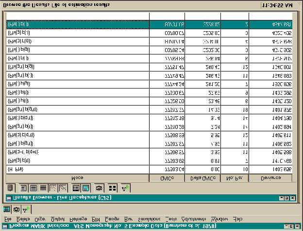
Results Browser
The Results Browser Window (Fig. 4) allows you to examine output from models which you
have previously generated and stored in the Results file. The Results file holds the results of previous
model runs. The file is a dBASE file, with memo fields to hold the numerical estimation output and the
residuals from the model. The Results file is named with the same root name as the input file used to
create it, but with the DBF extension. In addition, an FPT file is created to hold the memo fields
(output and residuals), and a CDX file holds the index orderings (Model Name, QAICc, Number of
Parameters, and Deviance). Keep these 3 files (DBF, FPT, and CDX) together. Once the results file
has been created, the input file containing the encounter histories is no longer necessary, as this
information has been stored in the result file.
The Results Browser displays a summary table of model results, including the Model Name,
QAICc, Delta QAICc, and Deviance. QAICc is computed as
− 2 log( Likelihood) 2 K ( K + 1)
) + 2K + ,
c n− K −1
)
where c is the quasi-likelihood scaling parameter, K is the number of parameters estimated and n is
the effective sample size. The Delta QAICc is the difference in the QAICc of the current model and
the model with the minimum QAICc. Deviance is the difference in the -2log(Likelihood) for the
current model and the saturated model (model with a parameter for every unique encounter history).
In addition, the numerical output for the model is included in a memo field in the Results data base, and
can be viewed by clicking on the Output, Specific Model, NotePad menu choices. Other menu options
allow you to retrieve a previous model, including the Parameter Index Matrices (PIM) and Design
Matrix, for creating a new model, to print the numerical output from a model to the printer, to produce
a table of the model summary statistics in a NotePad Window, and to graphically display the deviance
residuals (Fig. 5) or Pearson residuals for a particular model. With observed (O) and expected (E)
values for each capture history, a deviance residual is defined for each capture history as: sign(O - E)
)
sqrt{2 [E - O + O log(O/E)] / c }, where sign is the sign (plus or minus) of the value of O - E, sqrt is
)
square root, and log is the natural log. The value of c is the over dispersion scale parameter, and is
)
normally taken as 1. A Pearson residual is defined as (O - E) / sqrt(E c ). To see which observation
is causing a particular residual value, place your mouse cursor on the plotted point for the residual, and
click the left button. A description of this residual will be presented, including the attribute group that
the observation belongs to, the encounter history, the observed value, the expected value, and the
residual value. The horizontal dashed lines across the graph in Fig. 5 indicate ± 196 . , i.e., the area
within which 95% of the residuals would be distributed if they were normally distributed.Program MARK: Survival Estimation from Populations of Marked Animals 22
Other menu options are available to change the quasi-likelihood scaling parameter ( c ) ), or
modify the number of parameters identifiable in the model (which changes the QAICc value).
For any model shown in the Results Browser window, and for which the variance-covariance
matrix was computed, the variance components estimators described by Burnham can be computed,
and a graph of the results produced. You are asked to specify a set of parameters for which the
shrinkage estimators are to be computed, and the assumed model structure for the expected
parameters. Three choices of model structures are provided: constant or mean, linear trend, and a
user-specified model that could include covariates. Variance components estimation is mainly used for
a parameter type if that parameter is estimated under a time-saturated model. Variation across many
attribute groups might also be reasonably estimated, i.e., some form of random effects model.
Under the Tests menu selection, you can construct likelihood ratio and ANODEV tests, plus
evaluate the probability level of chi-square and F statistics. To construct likelihood ratio tests, you can
select 2 or more models, and tests between all pairs of the models selected will be computed. The user
must ensure that the models are properly nested to obtain valid likelihood ratio tests.
ANODEV provides a means of evaluating the impact of a covariate by comparing the amount of
deviance explained by the covariate against the amount of deviance not explained by this covariate.23, 45
For Analysis of Deviance (ANODEV) tests, the user must select 3 models:
Global model: model with largest number of parameters that explains the total deviance,
Covariate model: model with the covariate that you want to test, and
Constant model: model with the fewest number of parameters that explains only the mean level of
the effect you are examining.
As an example, to compute the ANODEV for survival with a linear trend {S(T)} model, you would
specify the Covariate model as {S(T)}, the Global model as {S(t)}, and the Constant model as {S(.)}.
The 3 models you select will automatically be classified based on their number of parameters as the
Global, Covariate, and Constant models. If the 3 models you select are not properly nested to form the
ANODEV, MARK will not tell you because it has no way of knowing this information. The program
uses the number of parameters of each model to determine which is which. No check to identify
improper nesting is provided.
NUMERICAL ESTIMATION PROCEDURES
Program MARK computes the log(Likelihood) based on the encounter histories:
No.UniqueEncounter Histories
log(Likelihood) = ∑ log[Pr(Observing this Encounter History)]
1
× No. Of Animals with this Encounter History .
The Pr(Observing this Encounter History) is computed by parsing the encounter history, equivalent to
the procedure demonstrated by Burnham32 in his Table 2. Identical encounter histories are grouped to
minimize computer time, except when individual covariates preclude grouping identical histories.
Numerical optimization based on a quasi-Newton approach is used to maximize the likelihood.
Initial parameter estimates are needed to start this process. The design matrix is assumed to be anProgram MARK: Survival Estimation from Populations of Marked Animals 23
identity matrix if no design matrix is specified. With all parameters in the β vector set to zero for the
sin link function, the resulting initial value of each parameter estimate (i.e., φ, p, S , r etc.) is 0.5. The
first step is to optimize the likelihood using the sin link function to obtain a set of estimates for β .
These estimates are then transformed with a linear matrix transformation to obtain approximate
estimates for the desired link function if it is not the sin. Optimization continues with the desired link
function to obtain final estimates of β .
Unequal time intervals between encounter occasions are handled by taking the length of the time
interval as the exponent of the survival estimate for the interval, i.e., Si L . This approach is also used
for φi and Fi because both of these basic parameters apply to an interval. For the typical case of
equal time intervals, all unity, this function has no effect. However, suppose the second time interval is
2 increments in length, with the rest 1 increment. This function has the desired consequences: the
survival estimates for each interval are comparable, but the increased span of time for the second
interval is accommodated. Thus, models where the same survival probability applies to multiple
intervals can be evaluated, even though survival intervals are of different length. This technique is
applied to all models where the length of the time intervals varies.
The information matrix (matrix of second partial derivatives of the likelihood function) is
computed with the method specified by the user. The singular value decomposition of this matrix is then
performed via LINPACK subroutine DSVDC 46 to obtain its pseudo-inverse (variance-covariance
)
matrix of β ) and the vector of singular values arranged in descending order of magnitude. The
number of estimable parameters is taken as the rank of the information matrix, determined by inspecting
the vector of singular values. If the smallest singular value is less than a criterion value specific for each
method of computing the variance-covariance matrix, the matrix is considered to not be full rank. Then
the maximum ratio of consecutive elements of this vector is determined. The rank of the matrix is taken
as the number of elements in the vector above this maximum ratio. In the case of a (declared) singular
information matrix, the parameter corresponding to the smallest singular value is identified in the output,
so that the user can provide additional constraints on the model to remove the inestimable parameters, if
desired. One option is to fix the parameter to a specific value.
)
The variance-covariance matrix of β is then converted to the variance-covariance matrix of the
estimated parameters ( θ ) specified in the PIMs based on the delta method, which is the same as
)
obtaining the information matrix for θ and inverting it. Likewise, the estimates of β are converted to
)
estimates of parameters specified in the PIMs, i.e. θ . For problems that include individual covariates,
the estimates for the back-transformed parameters are for the first individual listed in the input file after
the encounter histories are sorted into ascending order.
OPERATING SYSTEM REQUIREMENTS
Windows 95 is required to run Program MARK. No other special software is required.
However, because of the large amount of numerical computation needed to produce parameter
estimates, a fast Windows 95 computer is desirable. There are no fixed limits on the maximum number
of parameters, encounter occasions, or attribute groups. The more memory available, the larger theYou can also read