Effects of Displacement from Marine Renewable Development on Seabirds Breeding at SPAs: A Proof of Concept Model of Common Guillemots Breeding on ...
←
→
Page content transcription
If your browser does not render page correctly, please read the page content below
Effects of Displacement from Marine
Renewable Development on Seabirds
Breeding at SPAs:

A Proof of Concept Model of Common
Guillemots Breeding on the Isle of May
Final report to MSS
May 2012
Effects of displacement from marine renewable development

              on seabirds breeding at SPAs:

 a proof of concept model of common guillemots breeding
                     on the Isle of May

                    Final report to MSS

                        May 2012

   Claire McDonald, Kate Searle, Sarah Wanless & Francis
   Daunt

                      CEH Edinburgh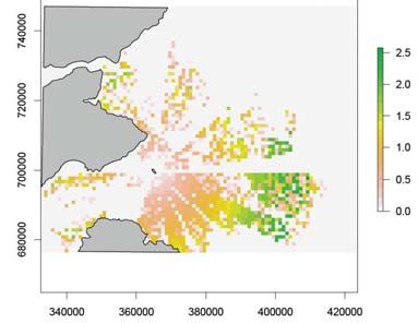
Contents

1.   Introduction                                    1
     1.1. Background                                 1
     2.1. Aims & Objectives                          1

2.   Methods                                         2
     2.1. Study Area and Species                     2
     2.2. Simulation Model                           3
            2.2.1. Input layers                      4
            2.2.2. Guillemot behaviour               7
            2.2.3. Wind farm presence                9
            2.2.4. Model Output                     10
     2.3. Cost Model                                11
            2.3.1. Flight Cost                      11
            2.3.2. Foraging Cost                    11
            2.3.3. Wind farm specific costs         13
     2.4. Scenarios                                 14
     Result
3.   s                                              15
     3.1. Random prey density                       15
     3.2. Clustered prey                            23
     3.3. Increased Interference Coefficient        30

4.   Discussion                                     37
     4.1. Displacement model                        37
     4.2. Population consequences of displacement   39

5.   Conclusions                                    41

6.   Acknowledgements                               41

7.   References                                     42

8.   Appendix 1                                     46
List of Figures

Figure 1. The three simulation model input layers required. a) Prey density                6
distribution – scale bar is number of prey individuals.

Figure 2. The 11 sectors (blue polygons) used in the simulation model to represent         7
the distribution of guillemot flight directions from the Isle of May.

Figure 3. The prey density map used in the simulation model with a halo of reduced         8
prey density shown in the circled area.

Figure 4. The location of the Neart na Gaoithe wind farm (red polygon) and the 5km         9
buffer zone (white polygon) used in the simulation model.

Figure 5. The clustered prey distribution used in Scenario 2 to represent prey items      10
as a shoal. Scale bar is the number of individuals in each cell.

Figure 6. The mean number of guillemots within each cell of the simulation model          17
using a random prey density distribution from 50 simulations with a) no wind farm
and b) with a wind farm.

Figure 7. The standard deviation of the mean number of guillemots within each cell        18
from 50 simulations with a random prey density distribution: a) no wind farm and b)
with a wind farm.

Figure 8. The mean flight cost incurred at each cell after 50 simulations of the model    19
with a random prey density distribution layer and with a) no wind farm and b) with a
wind farm present.

Figure 9. The mean foraging cost incurred at each cell after 50 simulations of the        20
model with a random prey distribution layer and with a) no wind farm and b) with a
wind farm present.

Figure 10. The distribution of flight costs incurred for 50 simulations of 1000 birds     21
with a random prey density layer: a) without a wind farm present and b) with a wind
farm present.

Figure 11. The distribution of foraging costs incurred for 50 simulations of 1000         22
guillemots with a random prey density layer: a) without a wind farm present and b)
with a wind farm present.

Figure 12. The mean number of guillemots within each cell of the simulation model         24
using a clustered prey density map from 50 simulations with a) no wind farm and b)
with a wind farm.

Figure 13. The standard deviation of the mean number of guillemots within each cell       25
from 50 simulations with a clustered prey density distribution: a) no wind farm and
b) with a wind farm.

Figure 14. The mean flight cost incurred at each cell after 50 simulations of              26
The model with a clustered prey density distribution layer and with a) no wind farm and b)
with a wind farm present.
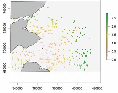
Figure 15. The mean foraging cost incurred at each cell after 50 simulations of the 27
model with a clustered prey distribution layer and with a) no wind farm and b) with a
wind farm present.

Figure 16. The distribution of flight costs incurred for 50 simulations of 1000 birds   28
with a clustered prey density layer: a) without a wind farm present and b) with a
wind farm present.

Figure 17. The distribution of foraging costs incurred for 50 simulations of 1000       29
guillemots with a clustered prey density layer: a) without a wind farm present and b)
with a wind farm present.

Figure 18. The mean number of guillemots within each cell of the simulation
model                                                                                   31
using a random prey density map and a high interference coefficient from 50
simulations with a) no wind farm and b) with a wind farm.

Figure 19. The standard deviation of the mean number of guillemots within each cell     32
from 50 simulations with a random prey density distribution and an increased
interference coefficient: a) no wind farm and b) with a wind farm.

Figure 20. The mean flight cost incurred at each cell after 50 simulations of the       33
model with a random prey density distribution layer, an increased interference
coefficient and with a) no wind farm and b) with a wind farm present.

Figure 21. The mean foraging cost incurred at each cell after 50 simulations of the     34
model with a clustered prey distribution layer and with a) no wind farm and b) with a
wind farm present.

Figure 22. The distribution of flight costs incurred for 50 simulations of 1000 birds   35
with a random prey distribution layer and an increased interference coefficient: a)
without a wind farm present and b) with a wind farm present.

Figure 23. The distribution of foraging costs incurred for 50 simulations of 1000       36
guillemots with a random prey distribution layer and an increased interference
coefficient: a) without a wind farm present and b) with a wind farm present.

Figure 24. Flow diagram illustrating the linking of time-energy budget and              39
population models to estimate population consequences of displacement.
Executive Summary

•   Offshore renewable developments have the potential to impact on seabirds by
    displacing individuals from foraging habitats. The impact of displacement is
    particularly important for breeding seabirds that, as central place foragers, are
    constrained to obtain food within a certain distance from the breeding colony. The
    current worst case scenario is that displacement causes 100% mortality, so there is
    a need to model more realistic consequences of displacement.
•   Displacement is likely to result in changes to daily energy and time budgets. Such
    changes may impact on the body condition of adult breeders which, in turn, can
    affect breeding success, adult survival and, ultimately, population size.
    Additionally, breeding success may be affected directly if provisioning rates alter
    significantly.
•   The Forth and Tay Offshore Wind Developers Group (FTOWDG) have exclusivity
    licences for proposed wind farm developments in the outer Forth and Tay which
    are offshore from a suite of SPAs for seabird species that will potentially interact
    with these developments. As part of the environmental evaluation of these
    developments there is a need to assess the potential impacts of displacement on
    breeding birds.
•   This report presents a displacement model for adult common guillemots Uria
    aalge rearing chicks on the Isle of May (part of Forth Islands SPA) in relation to
    the proposed offshore wind farm at Neart na Gaoithe. The model estimates the
    consequences of displacement and barrier effects on the time/energy budget of
    breeding birds.
•   Our model incorporates several novel features resulting in a step change in the
    degree of realism captured in terms of incorporating how guillemots use their
    foraging landscape and in how their fish prey are distributed within it.
•   The model compares the time/energy budget of 1,000 breeding guillemots over a
    24 hour period in the absence or presence of a wind farm. The model is based on
    assumptions regarding behavioural change in response to a wind farm and
    explores scenarios simulating different prey distributions (dispersed or patchy)
    and different levels of interference competition among guillemots feeding in the
    same patch.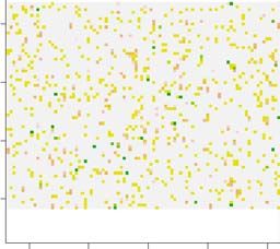
Under all scenarios, the presence of the Neart na Gaoithe wind farm resulted in an
increase in the average costs of foraging. For example, where prey were randomly
distributed, mean flight and foraging costs in the absence of the wind farm were 1.18 h
(± 0.60 h) and 2.19 h (± 0.96 h) respectively; equivalent values in the presence of the
wind farm were 1.60 (±0.67) and 2.58 (± 1.57) respectively. Under this scenario, the
mean number of birds displaced was 101, and the wind farm was a barrier to
movement for 44 birds.
• The impact of displacement is driven by two main processes: 1) the increased
    travelling costs to the subset of the population that is displaced or for which the wind
    farm forms a barrier to movement, and 2) the reduction in average prey densities in
    the remaining habitat due to intensified intra-specific competition, affecting not just
    displaced birds but the population as a whole.
• These results indicate that displacement effects on seabird populations could be
    important and therefore merit further consideration. The most appropriate method
    of estimating the population consequences of displacement is to link time-energy
    budget models of foraging with population models under a range of plausible
    scenarios of displacement. The report describes a framework for undertaking this
    linked modelling based on three components:
         • A time-energy budget model in the absence of a wind farm which extends
             the model presented here to produce a cumulative profitability surface over
             the course of the breeding season from which consequences on adult
             survival and breeding success are estimated.
         • A time-energy budget model in the presence of a wind farm in which
             the consequences of displacement and barrier effects on
             demographic rates are quantified.
         • A stochastic time-specific matrix model which quantifies the population
             consequences of displacement in three steps: a) a retrospective analysis of
             population change in relation to environmental conditions; b) a forecasting
             analysis of predicted population change under scenarios of future
             environmental change which provides a baseline for c) the predicted
• In conclusion, our model demonstrates that displacement of foraging seabirds
    from an offshore wind farm could result in changes to their time/energy budgets
    with potential consequences for breeding performance and/or survival. It also lays
    the foundation for estimating population consequences of displacement by linking
    time-energy budget models of foraging with population models.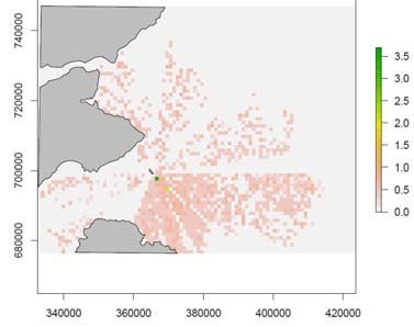
1. Introduction
1.1.   Background

Offshore renewable developments may have an effect on the daily energy and time
budgets of seabirds by displacing birds from favoured foraging habitats, potentially
forcing them to forage at greater densities in sub-optimal habitats (Larsen &
Guillemette 2007). The current worst case scenario is that displacement causes
100% mortality, so there is a need to model more realistic consequences of
displacement.

The impact of displacement is predicted to be particularly important for breeding
seabirds that, as central place foragers, are constrained to obtain food within a
certain distance from the breeding colony (Daunt et al. 2002; Enstipp et al 2006).
Changes in time and energy budgets resulting from displacement from a renewable
development have the potential to impact on the body condition, and hence survival
prospects, of breeding adults and also reduce breeding success because of changes
in provisioning rates. Both these outcomes could have population consequences and
thus need to be quantified, particularly where renewable developments are proposed
within the foraging range of breeding individuals from SPAs.

1.2.   Aims & Objectives

The aim of this project is to develop a displacement model for adult common
guillemots Uria aalge rearing chicks on the Isle of May (part of Forth Islands SPA) in
relation to the proposed offshore wind farm at Neart na Gaoithe. This site is one of a
suite proposed in the Forth/Tay region that currently also include Inch Cape and Firth
of Forth Zone 2. The model compares the time/energy budgets of breeding
guillemots in the absence of a wind farm, utilising available data on distribution and
activity budgets, with time/energy budgets in the presence of the wind farm, based
on plausible behavioural responses to the development.

                                          1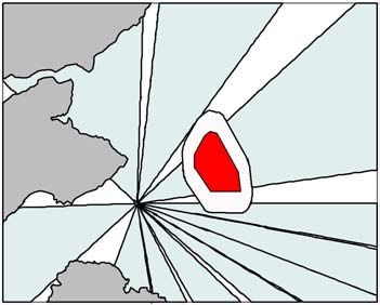
Our novel approach represents a significant advancement in our understanding of
the potential effects of displacement based on a step change in the degree of
realism captured by the model in terms of incorporating both:
    • how guillemots use their foraging landscape, both in the absence and
       presence of a wind farm, and
    • how their fish prey are distributed within it.
Thus, our model compares the effects of displacement when prey is dispersed or
patchy, and under elevated levels of interference competition among guillemots
feeding in the same patch (individuals may interfere with one another at higher
densities, resulting in lower prey capture rates, Hassell & Varley 1969).

In addition to presenting outputs from the model, this report discusses how the
model can be adapted to other species or locations and expanded in complexity to
parameterise population models that estimate the population consequences of
displacement.

2. Methods

2.1.   Study Area and Species

The Isle of May NNR, south-east Scotland (56°11’N, 02°33’W) is part of the Forth
Islands SPA (http://www.jncc.gov.uk/pdf/SPA/UK9004171.pdf). This SPA is
designated for its numbers of common guillemot (hereafter ‘guillemot’), razorbill
Alca torda, Atlantic puffin

Fratercula arctica, lesser black-backed gull Larus fuscus, northern gannet Morus
bassanus, European shag Phalacrocorax aristotelis, great cormorant P. carbo,
roseate tern Sterna dougallii, common tern S. hirundo and sandwich tern S.
sandvicensis.

This pilot study focused on one species for which a large body of empirical data exist
from the Isle of May, the guillemot. The guillemot is the third most numerous
breeding species in the Forth Islands SPA, after northern gannet and Atlantic puffin.
The population has been in sharp decline in the last decade from a peak in 2001 of

                                          2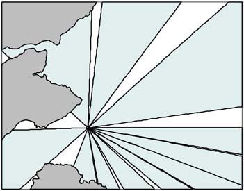
c. 30,000 pairs to the current population of ca. 18,000 pairs (Pickett & Squire 2011;
Bruce 2011). The guillemot is a pursuit-diving seabird that preys primarily on small,
shoaling fish such as lesser sandeels Ammodytes marinus and sprat Sprattus
sprattus (Harris & Wanless 1985; Wilson et al. 2004). It breeds in dense colonies on
cliff ledges, and both parents share the duty of incubation and rearing the single
offspring. Typically, one parent attends the young whilst the other is at sea.

There is a paucity of published data on the behaviour of breeding guillemots in
response to wind farms. The best current evidence on displacement is for non-
breeding individuals available from wind farm developments outside the UK. Studies
at Horns Rev wind farm, Denmark, suggest that guillemots did not forage in or travel
through wind farms (Petersen 2005). However, patterns were less clear cut at the
Egmond wind farm, off of the Dutch coast, with displacement recorded in some
situations but not others (Leopold et al 2011), and there was no evidence of
displacement of guillemots from Belgian developments (Vanermen et al. 2011). The
development of offshore wind farm sensitivity scores for seabirds (Garthe & Hüppop
2004) ranked guillemot 20th out of 26, although this low relative vulnerability score
was primarily due to the low collision risk for this species. Guillemots were scored as
moderate to high vulnerability for two of the factors most pertinent to displacement
(‘habitat use flexibility’ and ‘adult survival rate’). In accordance with this, the
guillemot was ranked 11th out of 38 in the list of species of concern due to
disturbance and/or displacement from habitat due to offshore wind farms by Furness
& Wade (2012). The inconsistent results obtained from empirical studies, paucity of
published information on displacement of breeding individuals, and moderate to high
vulnerability to displacement compared to other seabird species in the two reviews
on seabirds, highlight the importance of a displacement model for this species for
the outer Forth and Tay region.

2.2.   Simulation Model

A model was created to simulate the feeding location of 1000 guillemots (ca. 6% of
the SPA population) over a 24 hour period during chick-rearing (see Appendix 1 for
details of model input parameters including sources). The simulation model allowed
guillemots to choose the most suitable location for feeding during one foraging trip

                                           3
from the colony. The model incorporated realistic assumptions based on the known
behaviour of guillemots (Section 2.2.2.) to deduce what the best location would be.
The location of the 1000 guillemots and information on their chosen location are
stored for each simulation. The model incorporated the Isle of May and the
surrounding sea and land (OS Grid reference of bounding box of the model: xmin
332451 ymin 676319, xmax 423657, ymax 747098, area: 6532km2). The resolution
of the model was defined by the resolution of the input datasets (1 km2). The model
was run using the statistical software R v 2.14.1(R Development Core Team 2012).
2.2.1. Input layers
For the model to run successfully, three input layers were required (Figure 1): a prey
density distribution across the area, the bathymetry of the area (maximum possible
dive depth for the bird) and the distance of each location from the Isle of May (OS
Grid Reference 365679, 699182). The bathymetry of the area was obtained from the
British Geological Survey under licence (http://www.bgs.ac.uk/products/
offshore.html) and the distance of each location was calculated using the raster
package in R (Hijmans & van Etten 2012). The prey density distribution was
simulated using the rMatClust function in the R package spatstat (Baddeley & Turner
2005). This function generates a random number of points representing prey
individuals, such as lesser sandeels or sprat, inside the bounding box of the model.
The function also generates a Matérn’s cluster process which entails, for each point,
adding more points to create groupings of points. As the level of clustering
increases, more points occur within groups and distances increase between groups.
Unfortunately, no empirical data on fish shoal size and distribution were available for
use in the model, so it is uncertain how realistic is the clustering level selected for
examination here. However, it is likely that a clustered distribution is more realistic
than the random distribution. A grid is placed onto the surface of points and the
points summarised to create a prey density value for each 1km2 location. We used
linear distances, but note that this would underestimate distances for some areas,
notably in the Firth of Tay, which birds can not travel to directly.
4The input layers were used to create a set of rules to enable the simulated
guillemots to choose the best location to forage. The most suitable location was
defined as being less than 50km and greater than 0km from the Isle of May based
on empirically determined distributions of chick-rearing adults from animal-borne
instrumentation spanning several years (Wanless et al. 1990; 2000; 2005a; Thaxter
et al. 2009; 2010; Daunt et al. 2011a; b), the depth at the location had to be greater
than 0m (guillemots are entirely marine, Cramp 1985) and there had to be one or
more prey individuals at the location (for example, one or more lesser sandeels). If
more than one location met these criteria then the cells were ranked so that the
location that had the lowest dive depth, the smallest distance and highest prey
density was the one chosen (based on optimal foraging theory that individuals
would maximise gain and minimise cost, Stephens & Krebs 1986). The prey
density layer was updated after each guillemot had chosen a location to account for
prey being consumed and/or dispersed after feeding (Ashmole 1963; Lewis et al.
2001). The update was applied through the interference competition model of
Hassell & Varley 1969:
ai = Q*P-m
Where ai is the intake rate of an individual, Q is the intake rate achieved by a single
forager, P is the density of individuals at the site and m is interference coefficient.
The interference coefficient determined the strength of the density dependent
reduction in intake rate. For example, by increasing the interference coefficient, the
maximum intake rate achieved by an individual will be decreased. For the
simulation, Q was set at 0.4, P was taken from the number of guillemots at a
location in the simulation and m was set at 0.6. The values of Q and m were
obtained from both expert opinion and other interference competition studies on
birds (Ens and Goss-Custard 1984, Dolman et al. 1995, Goss-Custard et al. 1995).
5740000
a)
1600
1500
1400
1300
1200
720000
1100
Northing -BNG
1000
900
800
700
600
500
700000
400
300
200
100
0
680000
340000 360000 380000 400000 420000
Easting - BNG
740000
b)
70
60
720000
Northing - BNG
50
40
Isle of 30
700000
May 20
10
0
680000
340000 360000 380000 400000 420000
Easting - BNG
c)
740000
70000
60000
720000
Northing -BNG
50000
40000
30000
700000
20000
10000
680000
340000 360000 380000 400000 420000
Easting - BNG
2
Figure 1. The three simulation model input layers required each at 1km resolution and land is
shown in grey. a) Prey density distribution – scale bar is number of prey individuals. b) Bathymetry
data – scale bar is in depth (m), c) distance map layer – scale bar is the distance (m). Northings and
Eastings are in the British National Grid (BNG) reference system.
62.2.2. Guillemot behaviour
When guillemots fly away from the colony they typically do so on a bearing which
they continue to fly on until they reach their first foraging destination (Daunt et al.
2011a,b). This behaviour was incorporated into the model using the distribution of
empirical data on directions of guillemot flight for 159 trips from 54 individuals
recorded in 1999, 2002, 2003, 2005 and 2010 (Thaxter et al. 2009; 2010; Daunt et
al. 2011a; b). We considered it preferable to use empirical data on flight directions
than assume that flight direction was random. For each guillemot in the simulation, a
direction was sampled with replacement from the data. The summary statistics of the
flight direction distribution were then used to estimate a number of sectors to restrict
the flight path of guillemots in the simulation and, therefore, the feeding locations
potentially available to them on that foraging trip. A total of 11 sectors were created
in ArcMap v10 using the Sectors Tool (downloaded from the ESRI Mapping Centre).
This required the bearing, sector angle, radius and centre coordinates in latitude and
longitude for each sector. The sectors were different sizes to distribute the number
of different bearings evenly (Figure 2).
Figure 2. The 11 sectors (blue polygons) used in the simulation model to represent the
distribution of guillemot flight directions from the Isle of May. The grey polygons
represent the land.
7Guillemots depart the colony either singly or in flocks. Therefore, the simulation
code was adjusted to account for variation in the number of birds departing the
colony simultaneously. The estimates of flock size were based on data from 535
birds from colonies at Fowlsheugh and St. Abbs (Daunt et al. 2011c). The flock size
ranged from 1 to 50 birds and a negative binomial distribution was fitted to the data.
In the simulation, a flock size was sampled from this distribution and coupled to the
direction of flight. For example, if a guillemot left the colony on a bearing of 45o with
a flock size of 5, then the next 4 guillemots in the simulation would also need to find
a suitable location within the sector that incorporates 45o. After the five simulated
guillemots had chosen a location, the 6th bird would fly in a different direction.
It was assumed that when shoals were disturbed by the foraging activity of
guillemots, prey availability will be adversely affected, for example because shoal
size is reduced and/or the shoaling behaviour of the fish breaks down (Lewis et al.
2001). To incorporate this in the simulation model, an exponential decay function on
the effect of prey availability was added:
prey = exp(-λdij )
Where λ controls the level of the decay (decay constant) and dij is the distance
between points i and j. After exploring a range of decay rates using simulated data to
find the most appropriate effect distance (expert opinion), a decay rate of 0.001 was
used with the distance layer calculated previously to obtain a decay rate distribution
surface for the simulation. The decay rate distribution and the prey density layer are
multiplied together to obtain a halo (sensu Lewis et al. 2001) of reduced prey
availability around the Isle of May (Figure 3). For the set of input parameters used
here the halo effect was detectable up to a maximum distance of approximately 8km
from the Isle of May.
8740000
1600
1500
1400
BNG
1300
1200
1100
Northing
1000
-720000
900
800
700
600
500
400
700000
300
200
100
0
680000
Easting - BNG
340000 360000 380000 400000 420000
Figure 3. The prey density map used in the simulation model with a halo of reduced
prey density shown in the circled area. Scale bar is the number of individual prey within
a cell. Easting and Northing are in the British National Grid (BNG) reference system.
2.2.3. Wind farm presence
The simulation was modified to incorporate the presence of Neart na Gaoithe wind
farm within the model area (Figure 4). When a suitable foraging location was chosen
by a guillemot, then if that location was in the area of the wind farm as defined by
the red polygon (Figure 4), then the bird had to move to a new suitable location
within a 5km buffer zone of the wind farm (Figure 4). The assumption of the model
was that guillemots had no prior knowledge of the wind farm location and therefore
may fly out in the direction of the wind farm and will then need to feed in a suitable
location close by.
9Figure 4. The location of the Neart na Gaoithe wind farm (red polygon) and the 5km
buffer zone (white polygon) used in the simulation model. The grey polygons
represent land and the blue polygons mark out the sectors of bird flight direction.
2.2.4. Model Output
The simulation model produced a foraging location map of 1000 birds, the depth at
that location, the prey density at the location and the distance of the location from
the Isle of May. This information was used to calculate the flight and foraging cost
incurred by the guillemots (see Section 2.3). The simulation was repeated 50 times
to obtain a mean and standard deviation of guillemot locations. When the wind farm
was present within the model the number of birds that were displaced to a new
location was counted. In addition, the number of birds for which the wind farm acted
as a barrier to movement, either on their outward journey, return journey or both by
the wind farm, were recorded. It was assumed that birds would have to fly around
the wind farm, hence increasing the distance travelled and associated flight costs.
102.3. Cost Model
The output of the simulation model was used to calculate the time cost incurred by
the guillemots at their chosen feeding location. The cost model was an expanded
version of that used in Daunt & Wanless (2008) and Wanless et al. (1997). The cost
was separated into flight cost and foraging cost for each guillemot. The simulation
model generated information about one foraging trip per guillemot and the cost
incurred on this trip was multiplied by the average number of trips a guillemot makes
per day during chick-rearing (2.02 trips) to obtain a valid cost for a period of 24
hours. This estimate is based on empirical data from 2002-03 (Enstipp et al. 2006),
supported by a very similar value recorded in 1981-84 (Harris & Wanless 1985).
2.3.1. Flight Cost
The flight cost incurred by the guillemots was the time taken to travel the distance
both to and from the chosen location. This was calculated as the distance travelled
multiplied by 2 (assuming the same return path from the location) and divided by
the mean flight speed for a guillemot (19.1 ms-1; Pennycuick 1997).
2.3.2. Foraging Cost
The foraging cost calculated from the simulation was defined as the amount of time
the guillemots spend foraging to meet both the daily energy requirements of the
adult and 50% of the daily energy requirement of the offspring (assuming that two
parents share the costs of provisioning equally). Daily energy expenditure is
multiplied by the assimilation efficiency (0.78, Hilton et al. 2000b) to obtain the total
daily energy requirement of the guillemot.
The adult daily energy requirement is the total energy needed by the guillemot to fly
to the suitable location in the simulation plus the energy required carrying out other
activities such as resting on the sea surface and the length of time spent at the
colony. The time spent carrying out these activities was multiplied by activity-
specific energy costs taken from the literature (Flight energy cost: 7361.72 kJ day-1,
Pennycuick 1987, 1989; resting at sea energy cost: 810.28 kJ day-1, Croll &
McLaren 1993; time at colony energy costs: 1168.91 kJ day-1 Hilton et al. 2000a) .
The energy costs are then added to the cost of warming food (51.92 kJ, Grémillet
et al. 2003). The mean daily energy requirement of a guillemot chick was based on
provisioning rates recorded at this colony (221.71 kJ day-1, Harris & Wanless
111985). The daily energy requirement was converted into grams per day assuming a
mean energy density of 6.1 kJg-1 (Harris et al. 2008). Only total flight time could be
calculated from the output of the simulation model to estimate the daily energy
requirement. Therefore, the time spent resting at sea and at the colony was
estimated from the distribution of empirical data on activity budgets of 18 birds
(Wanless et al. 2005a). There are a number of sources of potential error when
calculating daily energy budgets. Activity specific costs are typically estimated in
captive studies, and it is possible that wild individuals are not equivalent.
Assimilation efficiency has also been estimated in captivity. The mean flight speeds
used in the calculation of flight costs may not be entirely accurate, and are likely to
vary among individuals dependent on environmental conditions (in particular wind
speed and direction). The mean energy density of prey is also expected to vary, as
demonstrated from analyses of interannual variation (Wanless et al. 2005b).
The amount of time guillemots spent foraging to meet their daily energy
requirements was assumed to depend on the prey availability at the chosen location.
This relationship was defined in the cost model by incorporating a functional
response between prey intake rate and prey density (Figure 5; Enstipp et al. 2007).
This relationship assumed a maximum prey intake rate of 5 g min-1 and that the
intake rate does not start to increase significantly until there is a prey density of 200
individuals per km2. A prey capture rate is obtained by multiplying the prey intake
rate by the diving efficiency. The diving efficiency was included to account for the
extra cost incurred with increased dive depth and it is obtained using the following
equation: (Daunt & Wanless 2008):
Dive efficiency = 0.36 – (0.0021 * dive depth (m))
The depth at the feeding location was obtained from the simulation and used in the
equation to calculate the diving efficiency. Using water depth at the location would
assume all dives were benthic. However, guillemots are known to forage throughout
the water column with a bimodal distribution of foraging depth (Daunt et al. 2006). To
allow for this, depth at the location for 50% of the birds was sampled from a normal
distribution with a mean of 11.71 m and a standard deviation of 8.07m (the
distribution was obtained using empirical data, Daunt & Wanless 2008). The prey
capture rate was then used to calculate the foraging time required by the bird to
meet half of the daily energy requirement (foraging for one trip). If the total foraging
time was greater than 12 hours for one trip then the birds would not be able to fulfil
their daily energy requirements.
122.3.3. Wind farm specific costs
The flight and foraging costs calculated for the simulation results with a wind farm
were the same as above, but with additional costs due to increased distance
travelled. The additional distance travelled between the first chosen suitable location
and the new location the guillemot was displaced to was included, as well as the
distance from the Isle of May to the first location on the outward journey and the
distance from the final location back to the Isle of May on the return journey. The
presence of the wind farm may not only displace birds to a new location, but may
also be a barrier to movement such that birds fly around it, therefore incurring
increased flight time. Guillemots with a final location beyond the wind farm, but which
were not displaced directly by the wind farm, had an additional outward distance to
travel. The additional outward cost was sampled from a normal distribution with a
mean of 20km and standard deviation of 5km due to the size of the wind farm (birds
would need to fly around the wind farm which would be approximately half of the
40km perimeter). Guillemots with a final location also beyond the wind farm, whether
they were displaced or not by the wind farm, would also incur an additional return
cost to fly around the wind farm. The return cost was also sampled from the same
distribution as the outward cost.
132.4. Scenarios
The simulation and cost models were run both with and without the presence of
the wind farm using the following scenarios:
1. The prey density layer was assumed to have a random distribution across
the model area (Figure 1a).
2. The prey density layer was changed to give a more clustered distribution
across the model area (Figure 5). The number of prey individuals across the
surface was the same as the random distribution, but the degree of
clustering was increased to give a more realistic representation of fish
shoals within the individual locations.
3. The interference coefficient in the simulation model was increased to 0.9 to
simulate more intense interference competition between foraging guillemots
that might occur if prey availability decreased.
740000
20000
720000
Northing -BNG
15000
10000
700000
5000
0
680000
340000 360000 380000 400000 420000
Easting - BNG
Figure 5. The clustered prey distribution used in Scenario 2 to represent prey items as a
shoal. Scale bar is the number of individuals in each cell. Northings and Eastings are in the
British National Grid (BNG) reference system.
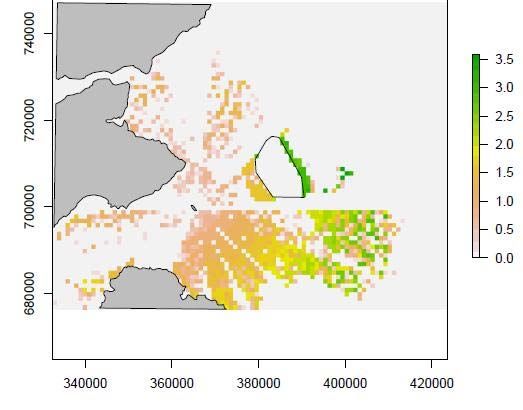
143. Results
3.1. Random prey density
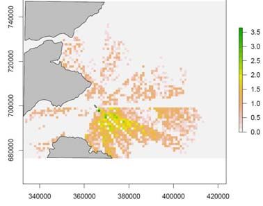
Using a random prey density distribution as an input layer in the simulation model
produced a mean distribution of birds per cell across the model space as shown in
Figures 6 and 7. In all results, the mean number given is from 50 simulations of 1000
birds in each run. The presence of the wind farm results in a higher density of birds
per cell with a particular increase in density of birds on the colony side of the wind
farm due to the birds being displaced. The flight and foraging costs increase with
increasing distance away from the Isle of May in simulation models both with and
without the wind farm (Figures 8 and 9 respectively). The guillemots incur increased
average flight costs (Figure 8) and foraging costs (Figure 9) when the wind farm is
present. The foraging costs for birds are higher on the colony side of the wind farm,
while the flight and foraging costs are higher on the far side. The higher flight costs
in Figure 8 are due to birds having to travel a longer distance. The higher foraging
costs in Figure 9 are due to an increase in the number of birds in one location which
leads to increased disturbance of prey, increased competition and hence, an
increase in foraging time to meet energy requirements. Mean flight and foraging
costs with and without the wind farm are presented in Table 1 and Figures 10 and 11
respectively.
Table 1. The mean flight and foraging costs for guillemots from the simulations under the three
scenarios tested. The summary results are from 50 simulations of 1000 birds.
Wind farm absent Wind farm present
Type of Scenario Mean cost /hours Mean cost /hours
Cost (± S.D.) (± S.D.)
Random prey 1.6
Flight 1.18 (± 0.60) 0 (±0.67)
1.5
Clustered prey
1.15 (± 0.67) 4 (±0.66)
Increased interference 1.5
coefficient 1.18 (± 0.61) 7 (±0.66)
2.5
Foraging Random prey 2.19 (± 0.96) (± 1.57)
8
Clustered prey 2.05 (± 0.85) 2.3 (± 1.16)
7
Increased interference
2.5
coefficient 2.21 (± 1.15) (± 1.81)
5
15When the wind farm was not present, the number of birds which do not meet their
energy requirements was 1.82 (±3.86) individuals (0.18%). When the wind farm was
present, 4.46 (± 7.19) guillemots could not meet their energy requirements (0.46%).
The mean number of birds that were displaced by the wind farm was 100.66 (±
28.00) individuals (10.07%). The mean number of birds which incurred additional
costs on their outward journey was 43.22 (±10.68) individuals and 45.18 (± 11.18)
individuals incurred additional costs on their return journey (4.32% and 4.52%
respectively).
16a)
BNG -
Northing
Easting - BNG
b)
-
BNG
Northing
Easting -BNG
Figure 6. The mean number of guillemots within each cell of the simulation model using a random
prey density distribution from 50 simulations with a) no wind farm and b) with a wind farm. The
scale bars are the number of guillemots per cell and the grey areas indicate land. The hollow
polygon indicates the wind farm position. Northings and Eastings are in British National Grid
reference system.
17a)
-
BNG
Northing
Easting - BNG
b)
BNG -
Northing
Easting - BNG
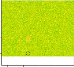
Figure 7. The standard deviation of the mean number of guillemots within each cell from 50
simulations with a random prey density distribution: a) no wind farm and b) with a wind farm.
The scale bars are the number of guillemots per cell and the grey areas indicate land. The
white polygon indicates the wind farm position. Northings sand Eastings are in the British
National Grid (BNG) reference system.
18a)
-
BNG
Northing
Easting -BNG
b)
-
BNG
Northing
Easting - BNG
Figure 8. The mean flight cost incurred at each cell after 50 simulations of the model with a
random prey density distribution layer and with a) no wind farm and b) with a wind farm
present. The scale bars are the number of hours spent in flight and the grey areas indicate
land. The hollow polygon indicates the wind farm position. Northings sand Eastings are in
the British National Grid (BNG) reference system.
19a)
-
BNG
Northing
Easting -BNG
b)
-
BNG
Northing
Easting - BNG
Figure 9. The mean foraging cost incurred at each cell after 50 simulations of the model
with a random prey distribution layer and with a) no wind farm and b) with a wind farm
present. The scale bars are the number of hours spent foraging and the grey areas
indicate land. The white polygon indicates the wind farm position. Northings and Eastings
are in the British National Grid (BNG) reference system.
20a) Without a wind farm
b) With a wind farm
Figure 10. The distribution of flight costs incurred for 50 simulations of 1000 birds with a
random prey density layer: a) without a wind farm present and b) with a wind farm present.
The bold line indicates the mean flight cost in hours and the dashed lines are the ±
standard deviations.
21a) Without a wind farm
b) With a wind farm
Figure 11. The distribution of foraging costs incurred for 50 simulations of 1000 guillemots
with a random prey density layer: a) without a wind farm present and b) with a wind farm
present.
223.2. Clustered prey
Using a more clustered prey density distribution that mimics the shoaling behaviour
of forage fish targeted by guillemots as an input layer in the simulation model,
produced a mean distribution of birds across the model space as shown in Figures
12 and 13. In all results, the mean number given is from 50 simulations of 1000 birds
in each run. Compared to the random prey density distribution model output, there is
an increase in the number of birds sharing each location (Figures 12 and 13). The
presence of the wind farm results in a higher density of birds per cell with particular
increase in density on the colony side of the wind farm due to the birds being
displaced. The flight and foraging costs increase with increasing distance away from
the Isle of May in simulation models both with and without the wind farm (Figure 14
and Figure 15 respectively). The higher flight costs in Figure 14 are due to birds
having to travel a longer distance. The higher foraging costs in Figure 15 are due to
an increase in the number of birds in one location which leads to increased
disturbance of prey, increased competition and hence, an increase in foraging time
to meet energy requirements. The frequency distribution of flight costs and foraging
costs for the guillemots are in Figures 16 and 17 and the flight and foraging costs
are summarised in Table 1.
When no wind farm is present, the mean number of birds which do not meet their
energy requirements was 6.76 (±3.93) individuals (0.68%). When the wind farm was
present, 7.66 (± 3.93) guillemots could not meet their energy requirements (0.77%).
The mean number of birds that were displaced by the wind farm was 103.34 (±
29.65) individuals (10.33%). The mean number of birds which incurred additional
costs on their outward journey and return journey were both 15.10 (±5.72)
individuals (1.51%).
Compared to the cost results for the random prey density distribution, the mean
flight costs and mean foraging costs were marginally lower when a clustered prey
density distribution was used. The presence of the wind farm caused an increase in
the mean flight and foraging cost for the clustered prey distribution scenario.
23a)
-
BNG
Northing
Easting - BNG
b)
-
BNG
Northing
Easting - BNG
Figure 12. The mean number of guillemots within each cell of the simulation model
using a clustered prey density map from 50 simulations with a) no wind farm and b) with
a wind farm. The scale bars are the number of guillemots per cell and the grey areas
indicate land. The hollow polygon indicates the wind farm position. Northings and
Eastings are in the British National Grid (BNG) reference system.
24a)
-
BNG
Northing
Easting - BNG
b)
-
BNG
Northing
Easting - BNG
Figure 13. The standard deviation of the mean number of guillemots within each cell
from 50 simulations with a clustered prey density distribution: a) no wind farm and b) with
a wind farm. The scale bars are the number of guillemots per cell and the grey areas
indicate land. The hollow polygon indicates the wind farm position. Northings and
Eastings are in the British National Grid (BNG) system.
25a)
-
BNG
Northing
Easting –BNG
b)
-
BNG
Northing
Easting - BNG
Figure 14. The mean flight cost incurred at each cell after 50 simulations of the model
with a clustered prey density distribution layer and with a) no wind farm and b) with a
wind farm present. The scale bars are the number of hours in flight and the grey
areas indicate land. The hollow polygon indicates the wind farm position. Northings
and Eastings are in the British National Grid (BNG) reference system.
26a)
-
BNG
Northing
Easting - BNG
b)
–BNG
Northing
Easting - BNG
Figure 15. The mean foraging cost incurred at each cell after 50 simulations of the model with a
clustered prey distribution layer and with a) no wind farm and b) with a wind farm present. The
scale bars are the number of hours spent foraging and the grey areas indicate land. The hollow
polygon indicates the wind farm position. Northings and Eastings are in the British National Grid
(BNG) reference system.
27a) No wind farm present
b) With a wind farm present
Figure 16. The distribution of flight costs incurred for 50 simulations of 1000 birds with a
clustered prey density layer: a) without a wind farm present and b) with a wind farm present.
28a) No wind farm present
b) With a wind farm present
Figure 17. The distribution of foraging costs incurred for 50 simulations of 1000 guillemots with a
clustered prey density layer: a) without a wind farm present and b) with a wind farm present. The bold
line indicates the mean foraging cost in hours and the dashed lines are the ± standard deviations.
293.3. Increased Interference Coefficient
The simulation using an increased interference coefficient in the simulation model
produced a mean distribution of birds per cell across the model space as shown in
Figures 18 and 19. In all results, the mean number given is from 50 simulations of
1000 birds in each run. Compared to the random prey density distribution model
output, there is an increase in the number of birds sharing each location (Figures 18
and 19). The presence of the wind farm results in a higher density of birds per cell
particularly on the colony side of the wind farm due to the birds being displaced.
Flight and foraging costs increase with increasing distance away from the Isle of May
in simulation models both with and without the wind farm (Figure 20 and 21
respectively). The foraging cost for guillemots are higher on the colony side of the
wind farm, but the flight and foraging costs are higher on the far side of the wind
farm. The higher flight costs in Figure 20 are due to birds having to travel a longer
distance. The higher foraging costs in Figure 21 are due to an increase in the
number of birds in one location which leads to increased disturbance of prey,
increased competition and hence, an increase in foraging time to meet energy
requirements. The frequency distribution of flight costs and foraging costs for the
guillemots in the simulation with and without the wind farm are shown in Figures 22
and 23. The flight and foraging costs for simulations both with and without a wind
farm are summarized in Table 1.
With no wind farm, the mean number of birds which do not meet their energy
requirements was 2.40 (±5.15) individuals (0.24%). When the wind farm was
present, 5.86 (± 7.07) individuals could not meet their energy requirements
(0.59%). The mean number of birds displaced by the wind farm was 83.84 (±
27.84) individuals (8.38%). The mean number of birds incurring additional costs
was 38.02 (± 9.69) individuals on the outward journey and 39.40 (±10.16)
individuals on their return journey (3.80% and 3.94% respectively).
The increased interference coefficient scenario produced similar flight costs to the
scenario with a lower interference coefficient. With no wind farm, the mean
number of hours spent foraging is greater with an increased interference
coefficient, but when the wind farm is present there is no difference in the mean
number of hours spent foraging.
30a)
-
BNG
Northing
Easting -BNG
b)
-
BNG
Northing
Easting -BNG
Figure 18. The mean number of guillemots within each cell of the simulation model
using a random prey density map and a high interference coefficient from 50
simulations with a) no wind farm and b) with a wind farm. The scale bars are the
number of guillemots per cell and the grey areas indicate land. The hollow polygon
indicates the wind farm position. Northings and Eastings are in the British National Grid
(BNG) reference system.
31a)
-
BNG
Northing
Easting - BNG
b)
-
BNG
Northing
Easting - BNG
Figure 19. The standard deviation of the mean number of guillemots within each cell
from 50 simulations with a random prey density distribution and an increased
interference coefficient: a) no wind farm and b) with a wind farm. The scale bars are the
number of guillemots per cell and the grey areas indicate land. The hollow polygon
indicates the wind farm position. Northings and Eastings are in the British National Grid
(BNG) reference system.
32a)
-
BNG
Northing
Easting - BNG
b)
BNG -
Northing
Easting -BNG
Figure 20. The mean flight cost incurred at each cell after 50 simulations of the model
with a random prey density distribution layer, an increased interference coefficient and
with a) no wind farm and b) with a wind farm present. The scale bars are the number of
hours in flight and the grey areas indicate land. The hollow polygon indicates the wind
farm position. Northings and Eastings are in the British National Grid (BNG) reference
system.
33a)
Northing BNG -
Easting -BNG
b)
Northing BNG -
Easting -BNG
Figure 21. The mean foraging cost incurred at each cell after 50 simulations of the model
with a clustered prey distribution layer and with a) no wind farm and b) with a wind farm
present. The scale bars are the number hours spent foraging and the grey areas indicate
land. The hollow polygon indicates the wind farm position. Northings and Eastings are in
the British National Grid (BNG) reference system.
34a) No wind farm present
b) With a wind farm present
Figure 22. The distribution of flight costs incurred for 50 simulations of 1000 birds with a
random prey distribution layer and an increased interference coefficient: a) without a wind
farm present and b) with a wind farm present.
35a) No wind farm present
b) With a wind farm present
Figure 23. The distribution of foraging costs incurred for 50 simulations of 1000 guillemots
with a random prey distribution layer and an increased interference coefficient: a) without a
wind farm present and b) with a wind farm present. The bold line indicates the mean
foraging cost in hours and the dashed lines are the ± standard deviations.
364. Discussion
4.1. Displacement model
The model presented in this report represents a significant step forward towards
understanding the implications of displacement and barrier effects of wind farms on
seabirds breeding at SPAs. To our knowledge, this is the first attempt to model how
breeding individuals in a seabird population use their foraging landscape, and,
crucially, how this changes when a component of the population is displaced or has
to travel round a wind farm development.
In all scenarios, the addition of the Neart na Gaoithe wind farm resulted in an
increase in the average costs of foraging. This result is important since it suggests
that displacement effects merit further consideration. The impact of displacement
was driven by two main processes:
• the increased travelling costs incurred by the subset of the population that is
displaced or for which the wind farm forms a barrier to movement, and
• the reduction in average prey densities in the remaining habitat due to
intensified intra-specific competition, affecting not just displaced birds but
the population as a whole.
Whilst there were some differences amongst the scenarios tested, the effect of the
wind farm on time/energy budgets was consistent, suggesting that the
displacement effect was apparent at different levels of prey aggregation and
degrees of interference between individual guillemots.
Whilst the number of birds that did not achieve their daily energy requirements in the
scenarios was comparatively small, the purpose of this project was to provide a proof
of concept of the modelling approach. As such, formal examination of the absolute
values is not justified since various aspects of the model are not realistic (e.g. 24
hour duration, population density). Future work would focus on developing the
approach to explore patterns across a whole season for the SPA population as a
whole. The potential effects of displacement over these time scales are hard to
predict from the values presented in the model, since the relationships are unlikely to
be linear, and may involve a range of outcomes - see section 4.2 part 2).
37Although we used the Isle of May guillemot population and the Neart na Gaoithe
wind farm to showcase the model, the framework is extremely flexible and could
readily be updated, for example to take advantage of improved data on foraging
behaviour or prey distribution. Similarly it could be adapted for different seabird or
prey species by incorporating appropriate information on foraging behaviour and
distribution respectively. Moreover, this model could be adapted to situations where
no empirical data are available (e.g. flight direction could be modelled as random),
subject to the appropriate caveats. The model could also be scaled up to the whole
SPA, and incorporate interannual and seasonal variation including the effects of
displacement on wintering birds. With further development, it could also explore
outcomes for multiple species simultaneously, enabling inter- as well as intra-
specific competition to be accounted for in the calculations. This modification is likely
to be particularly insightful since seabird breeding colonies typically comprise
several species and inter-specific facilitation and competition among multi-species
feeding flocks are well known. Finally alternative scenarios of array location and
design could be explored within this framework, and identifying designs that maintain
energy balance above a defined threshold (e.g. that maintained population level
effects below a threshold as agreed in consultation with interested parties – see next
section) could be particularly useful, while sensitivity analyses could be employed to
identify minimum data requirements and highlight priorities for future monitoring. The
model could also be adapted to other case studies, and is designed so that
cumulative effects from multiple developments could be estimated, with a view of
informing marine spatial planning as well as decisions on a case by case basis.
Changes in the time/energy budgets of breeding seabirds can have important
population consequences. This is because such changes may impact on the body
condition of adult breeders which, in turn, can affect breeding success (through
abandonment of young), adult survival and, ultimately, population size.
Additionally, breeding success may be affected directly if provisioning rates alter
significantly. There is an urgent need to estimate these more realistic population
consequences of displacement, to provide improved assessments of likely adverse
effects on SPA populations. Below, we describe how the outputs of the model can
be used to parameterise population models that estimate the population
consequences of displacement.
384.2. Population consequences of displacement
The most appropriate method of estimating the population consequences of
displacement is to link time-energy budget models of foraging with population
models under a range of plausible scenarios of displacement (Figure 24).
Time-energy budget model Population model
Foraging gain / Foraging cost Retrospective analysis
= Foraging profitability of past demography
Cumulative seasonal Forecasting of
time + energy balance future demography
Breeding Adult
success survival
Forecasting displacement effect
on demography
Figure 24. Flow diagram illustrating the linking of time-energy budget and population
models to estimate population consequences of displacement.
The framework can be split into three components:
1) Time-energy budget model: The time-energy model in the absence of a
wind farm, presented in this report over a 24 hour period, would be expanded into
a cumulative profitability surface estimated over the course of the breeding
season. This seasonal model would be quantified in a range of environmental
conditions from optimum to severe, based on the range of conditions experienced
in the region and forecasted in climate models.
39Sustained time/energy deficits may have consequences both for breeding success
and adult survival, two critical drivers of population dynamics. Life history theory
predicts a trade-off between investment in current breeding and self-maintenance
(Ylönen et al. 1998). Available data on the relationships between energy balance
and these two parameters would be utilised; alternatively, theoretical understanding
would be used (e.g. allometric scaling relationships). To breed successfully, one
member of a pair of most species of seabird, including guillemots, needs to be
constantly present at the nest site. Thus, increased time required for foraging can
result in temporary unattendance of eggs or young which increases the likelihood of
failure (Harris & Wanless 1997; Ashbrook et al. 2008). These fitness consequences
of time and energy budgets underpin the subsequent displacement scenarios.
2) Consequences of displacement on breeding success and adult survival: The
impact of changes in time/energy budgets on breeding success and adult survival
would be estimated using the same approach as the baseline time-energy budget
model. There are a number of challenges in reaching a satisfactory conclusion,
given the lack of information on fitness consequences of foraging energetics and the
effects of displacement on these parameters. Thus, where possible available
empirical data would be used, or theoretical understanding together with experience
of the species’ ecology. At this stage, the most appropriate set of outcomes (for
each set of environmental conditions) may be a matrix of severity against likelihood.
3) Population consequences of displacement. A stochastic time-specific matrix
model (Caswell 2001; Frederiksen et al. 2008) using data on breeding success and
adult survival and, where available, on age at first breeding, age structure and
juvenile survival would quantify the population consequences of displacement. The
modelling would be undertaken in three steps:
a. Retrospective analysis: existing time would be evaluated to assess how
well they capture observed historical population trends, and what
environmental variables correlate with demographic rates.
b. Forecasting population change: models would simulate future population
growth rate. These simulations would be driven by change in breeding
success and adult survival resulting from predicted environmental change
or current trends where possible, or in the absence of these the
distribution of historical parameter values.
40You can also read